Optimally sparse approximations of 3D functions by compactly supported shearlet frames

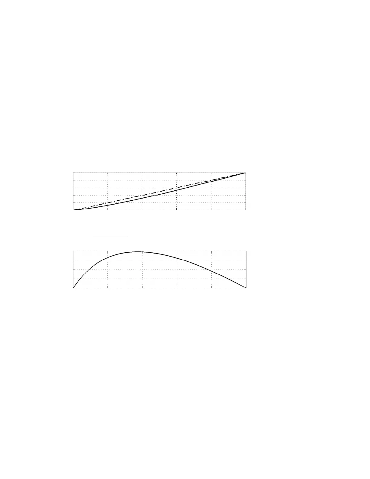
OPTIMALL Y SP ARSE APPR O XIMA TIONS OF 3D FUNCTIONS BY COMP A CTL Y SUPPOR TED SHEARLET FRAMES GITT A KUTYNIOK ∗ , JAKOB LEMVIG † , AND W ANG-Q LIM ‡ Abstract. W e study eﬃcien t and reliable metho ds of capturing and sparsely representing aniso- tropic structures in 3D data. As a model class for multidimensional data with anisotropic features, we introduce generalized three-dimensional carto on-lik e images. This function class will hav e tw o smoothness parameters: one parameter β controlling classical smo othness and one parameter α controlling anisotropic smo othness. The class then consists of piecewise C β -smooth functions with discontin uities on a piecewise C α -smooth surface. W e introduce a pyramid-adapted, hybrid shearlet system for the three-dimensional setting and construct frames for L 2 ( R 3 ) with this particular shearlet structure. F or the smo othness range 1 < α ≤ β ≤ 2 we show that pyramid-adapted shearlet systems provide a nearly optimally sparse approximation rate within the generalized carto on-like image mo del class measured by means of non-linear N -term appro ximations. Key words. anisotropic features, multi-dimensional data, shearlets, cartoon-like images, non- linear appro ximations, sparse approximations AMS sub ject classiﬁcations. Primary: 42C40, Secondary: 42C15, 41A30, 94A08 1. In tro duction. Recen t adv ances in mo dern technology ha ve created a new w orld of huge, multi-dimensional data. In biomedical imaging, seismic imaging, as- tronomical imaging, computer vision, and video pro cessing, the capabilities of mo d- ern computers and high-precision measuring devices hav e generated 2D, 3D and even higher dimensional data sets of sizes that were infeasible just a few years ago. The need to eﬃciently handle such div erse types and huge amounts of data has initiated an in tense study in developing eﬃcient multiv ariate encoding metho dologies in the applied harmonic analysis researc h communit y . In neuro-imaging, e.g., ﬂuorescence microscop y scans of living cells, the discontin uit y curves and surfaces of the data are imp ortan t sp eciﬁc features since one often wan ts to distinguish b et w een the image “ob- jects” and the “background”, e.g., to distinguish actin ﬁlaments in euk ary otic cells; that is, it is imp ortant to precisely capture the edges of these 1D and 2D structures. This sp eciﬁc application is an illustration that imp ortant classes of multiv ariate problems are gov erned by anisotr opic fe atur es . The anisotropic structures can be distinguished b y lo cation and orien tation or direction whic h indicates that our w ay of analyzing and represen ting the data should capture not only lo cation, but also directional infor- mation. This is exactly the idea b ehind so-called directional representation systems whic h by now are well developed and understo o d for the 2D setting. Since muc h of the data acquired in, e.g., neuro-imaging, are truly three-dimensional, analyzing suc h data should b e p erformed by three-dimensional directional representation systems. Hence, in this pap er, we therefore aim for the 3D setting. In applied harmonic analysis the data is typically mo deled in a contin uum setting as square-in tegrable functions or distributions. In dimension t wo, to analyze the abilit y of representation systems to reliably capture and sparsely represent anisotropic structures, Candés and Donoho [7] in tro duced the mo del situation of so-called carto on- ∗ T echnische Universität Berlin, Institut für Mathematik, 10623 Berlin, Germany , E-mail: kutyniok@math.tu- berlin.de † T echnical Universit y of Denmark, Department of Mathematics, Matematiktorv et 303, 2800 Kgs. Lyngby , Denmark, E-mail: J.Lemvig@mat.dtu.dk ‡ T echnische Univ ersität Berlin, Institut für Mathematik, 10623 Berlin, Germany , E-mail: lim@ math.tu- berlin.de 1 2 G. KUTYNIOK, J. LEMVIG, AND W.-Q LIM lik e images, i.e., t wo-dimensional functions whic h are piecewise C 2 -smo oth apart from a piecewise C 2 discon tinuit y curv e. Within this mo del class there is an optimal sparse appro ximation rate one can obtain for a large class of non-adaptive and adaptiv e represen tation systems. In tuitively , one should think adaptive systems would b e far sup erior in this task, but it has b een shown in recen t y ears that non-adaptive metho ds using curvelets, contourlets, and shearlets all hav e the abilit y to essentially optimal sparsely approximate carto on-lik e images in 2D measured by the L 2 -error of the b est N -term approximation [7, 13, 17, 24]. 1.1. Dimension three. In the present pap er we will consider sparse approxima- tions of carto on-like images using shearlets in dimension thr e e . The step from the one- dimensional setting to the tw o-dimensional setting is necessary for the app earance of anisotropic features at all. When further passing from the tw o-dimensional setting to the three-dimensional setting, the complexity of anisotropic structures c hanges signiﬁ- can tly . In 2D one “only” has to handle one type of anisotropic features, namely curv es, whereas in 3D one has to handle two geometrically very diﬀerent anisotropic struc- tures: Curves as one-dimensional features and surfaces as tw o-dimensional anisotropic features. Moreo v er, the analysis of sparse appro ximations in dimension tw o dep ends hea vily on reducing the analysis to aﬃne subspaces of R 2 . Clearly , these subspaces alw ays hav e dimension and co-dimension one in 2D. In dimension three, how ever, w e ha ve subspaces of co-dimension one and tw o, and one therefore needs to p erform the analysis on subspaces of the “correct” co-dimension. Therefore, the 3D analysis requires fundamental new ideas. Finally , w e remark that ev en though the present pap er only deals with the con- struction of shearlet frames for L 2 ( R 3 ) and sparse appro ximations of such, it also illustrates how many of the problems that arises when passing to higher dimensions can b e handled. Hence, once it is known how to handle anisotropic features of diﬀer- en t dimensions in 3D, the step from 3D to 4D can b e dealt with in a similar wa y as also the extension to even higher dimensions. Therefore the extension of the presented result in L 2 ( R 3 ) to higher dimensions L 2 ( R n ) should b e, if not straigh tforward, then at least b e achiev able by the metho dologies developed. 1.2. Mo delling anisotropic features. The class of 2D cartoon-like images consists, as mentioned ab ov e, of piecewise C 2 -smo oth functions with discontin uities on a piecewise C 2 -smo oth curv e, and this class has b een inv estigated in a num b er of recen t publications. The ob vious extension to the 3D setting is to consider functions of three v ariables b eing piecewise C 2 -smo oth function with discontin uities on a piecewise C 2 -smo oth surface. In some applications the C 2 -smo othness requireme n t is to o strict, and we will, therefore, go one step further and consider a larger class of images also con taining less regular images. The generalized class of cartoon-like images in 3D c on- sidered in this pap er consists of three-dimensional piecewise C β -smo oth functions with discon tinuities on a piecewise C α surface for α ∈ (1 , 2] . Clearly , this mo del provides us with tw o new smo othness parameters: β b eing a classical smo othness parameter and α b eing an anisotropic smo othness parameter, see Figure 1.1 for an illustration. This image class is unfortunately not a linear space as traditional smo othness spaces, e.g., Hölder, Besov, or Sob olev spaces, but it allows one to study the qualit y of the p erformance of represen tation systems with resp ect to capturing anisotropic features, something that is not p ossible with traditional smo othness spaces. Finally , w e mention that allowing pie c ewise C α -smo othness and not everywhere C α -smo othness is an essential w a y to mo del singularities along surfaces as wel l as along curves which we already describ ed as the tw o fundamental types of anisotropic APPRO XIMA TIONS OF 3D FUNCTIONS BY COMP ACTL Y SUPPOR TED SHEARLETS 3 ∂ B 0 1 4 1 2 3 4 1 0 1 4 1 2 3 4 1 0 1 4 1 2 3 4 1 Figure 1.1 . The support of a 3D c artoon-like image f = f 0 χ B , wher e f 0 is C β smo oth with supp f 0 = R 3 and the discontinuity surfac e ∂ B is pie c ewise C α smo oth. phenomena in 3D. 1.3. Measure for Sparse Appro ximation and Optimalit y . The quality of the p erformance of a represen tation system with respect to cartoon-like images is t ypically measured by taking a non-linear approximation viewp oin t. More precisely , giv en a carto on-lik e image and a representation system, the chosen measure is the asymptotic b eha vior of the L 2 error of N -term (non-linear) approximations in the n umber of terms N . When the anisotropic smo othness α is b ounded b y the classical smo othness as α ≤ 4 3 β , the anisotropic smo othness of the carto on-like images will b e the determining factor for the optimal appro ximation error rate one can obtain. T o b e more precise, as we will show in Section 3, the optimal appro ximation rate for the generalized 3D carto on-lik e images mo dels f which can b e achiev ed for a large class of adaptive and non-adaptiv e representation systems for 1 < α ≤ β ≤ 2 is k f − f N k 2 L 2 ≤ C · N − α/ 2 as N → ∞ , for some constant C > 0 , where f N is an N -term appro ximation of f . F or carto on-like images, wa velet and F ourier metho ds will t ypically hav e an N -term appro ximation error rate decaying as N − 1 / 2 and N − 1 / 3 as N → ∞ , resp ectiv ely , see [23]. Hence, as the anisotropic smoothness parameter α gro ws, the approximation qualit y of tradi- tional to ols b ecomes increasingly inferior as they will deliver approximation error rates that are far fr om the optimal rate N − α/ 2 . Therefore, it is desirable and necessary to searc h for new representation systems that can provide us with represen tations with a more optimal rate. This is where p yramid-adapted, hybrid shearlet systems enter the scene. As we will see in Section 6, this t yp e of represen tation system pro vides nearly optimally sparse appro ximations: k f − f N k 2 L 2 ≤ ( C · N − α/ 2+ τ , if β ∈ [ α, 2) , C · N − 1 (log N ) 2 , if β = α = 2 , ) as N → ∞ , where f N is the N -term approximation obtained b y k eeping the N largest shearlet co eﬃcien ts, and τ = τ ( α ) with 0 ≤ τ < 0 . 04 and τ → 0 for α → 1 + and for α → 2 − . Clearly , the obtained sparse appro ximations for these shearlet systems are not truly optimal owing to the p olynomial factor τ for α < 2 and the p olylog factor for α = 2 . 4 G. KUTYNIOK, J. LEMVIG, AND W.-Q LIM On the other hand, it still shows that non-adaptive sc hemes such as the hybrid shearlet system can provide rates that are nearly optimal within a large class of adaptive and non-adaptiv e metho ds. 1.4. Construction of 3D hybrid shearlets. Shearlet theory has b ecome a cen tral tool in analyzing and representing 2D data with anisotropic features. Shearlet systems are systems of functions generated by one single generator with parab olic scaling, shearing, and translation operators applied to it, in muc h the same wa y w av elet systems are dy adic scalings and translations of a single function, but includ- ing a directionality c haracteristic owing to the additional shearing op eration and the anisotropic scaling. Of the man y directional represen tation systems proposed in the last decade, e.g., steerable pyramid transform [29], directional ﬁlter banks [3], 2D directional w av elets [2], curvelets [6], con tourlets [13], bandelets [28], the shearlet sys- tem [25] is among the most versatile and successful. The reason for this b eing an extensiv e list of desirable prop erties: Shearlet systems can b e generated by one func- tion, they precisely resolv e wa v efront sets, they allow compactly supp orted analyzing elemen ts, they are associated with fast decomp osition algorithms, and they provide a uniﬁed treatment of the con tinuum and the digital realm. W e refer to [22] for a detailed review of the adv antages and disadv antages of shearlet systems as opp osed to other directional represen tation systems. Sev eral constructions of discrete band-limited and compactly supp orted 2D shear- let frames are already known, see [9, 11, 15, 20, 21, 26]; for construction of 3D shear- let frames less is kno wn. Dahlk e, Steidl, and T esc hke [10] recently generalized the shearlet group and the asso ciated con tinuous shearlet transform to higher dimensions R n . F urthermore, in [10] they show ed that, for certain band-limited generators, the con tinuous shearlet transform is able to identify h yp erplane and tetrahedron singu- larities. Since this transform originates from a unitary group representation, it is not able to capture all directions, in particular, it will not capture the delta distribution on the x 1 -axis (and more generally , any singularity with “ x 1 -directions”). W e will use a diﬀerent tiling of the frequency space, namely systems adapted to pyramids in frequency space, to av oid this non-uniformity of directions. W e call these systems p yramid-adapted shearlet system [22]. In [16], the con tinuous version of the pyramid- adapted shearlet system was introduced, and it was shown that the lo cation and the lo cal orien tation of the b oundary set of certain three-dimensional solid regions can be precisely identiﬁed by this contin uous shearlet transform. Finally , we will also need to use a diﬀeren t scaling than the one from [10] in order to achiev e shearlet systems that provide almost optimally sparse approximations. Since spatial lo calization of the analyzing elemen ts of the enco ding system is v ery imp ortant b oth for a precise detection of geometric features as well as for a fast decomp osition algorithm, we will mainly follo w the suﬃcient conditions for and construction of compactly supp orted cone-adapted 2D shearlets by Kittipo om and t wo of the authors [20] and extend these result to the 3D setting (Section 4). These results pro vide us with a large class of separable, compactly supp orted shearlet systems with “go o d” frame b ounds, optimally sparse appro ximation prop erties, and asso ciated n umerically stable algorithms. One imp ortan t new asp ect is that dilation will dep end on the smoothness parameter α . This will provide us with hybrid shearlet systems ranging from classical parab olic based shearlet systems ( α = 2 ) to almost classical w av elet systems ( α ≈ 1 ). In other words, we obtain a parametrized family of shearlets with a smooth transition from (nearly) w av elets to shearlets. This will allo w us to adjust our shearlet system according to the anisotropic smo othness of the data APPRO XIMA TIONS OF 3D FUNCTIONS BY COMP ACTL Y SUPPOR TED SHEARLETS 5 at hand. F or rational v alues of α we can asso ciate this h ybrid system with a fast decomp osition algorithm using the fast F ourier transform with m ultiplication and p eriodization in the frequency space (in place of con v olution and do wn-sampling). Our compactly supp orted 3D hybrid shearlet elements (introduced in Section 4) will in the spatial domain b e of size 2 − j α/ 2 times 2 − j / 2 times 2 − j / 2 for some ﬁxed anisotrop y parameter 1 < α ≤ 2 . When α ≈ 1 this corresp onds to “cub e-like” (or “w av elet-like”) elements. As α approaches 2 the scaling b ecomes less and less isotr opic yielding “plate-like” elements as j → ∞ . This indicates that these anisotropic 3D shearlet systems hav e been designed to eﬃciently capture tw o-dimensional anisotropic structures, but neglecting one-dimensional structures. Nonetheless, these 3D shearlet systems still perform optimally when representing and analyzing carto on-lik e func- tions that hav e discon tinuities on pie c ewise C α -smo oth surfaces – as mentioned suc h functions mo del 3D data that con tain b oth p oin t, curve, and surface singularities. Let us end this subsection with a general thought on the construction of band- limited tight shearlet frames versus compactly supp orted shearlet frames. There seem to b e a trade-oﬀ betw een c omp act supp ort of the shearlet generators, tightness of the asso ciated frame, and sep ar ability of the shearlet generators. The kno wn construc- tions of tight shearlet frames, even in 2D, do not use separable generators, and these constructions can b e sho wn to not b e applicable to compactly supported genera- tors. Moreov er, these tigh t frames use a mo diﬁed v ersion of the pyramid-adapted shearlet system in which not all elemen ts are dilates, shears, and translations of a sin- gle function. Tightness is diﬃcult to obtain while allowing for compactly supp orted generators, but we can gain separability as in Theorem 5.4 hence fast algorithmic realizations. On the other hand, when allowing non-compactly supp orted generators, tigh tness is p ossible, but separabilit y seems to be out of reach, whic h mak es fast algorithmic realizations very diﬃcult. 1.5. Other approaches for 3D data. Other directional represen tation systems ha ve b een considered for the 3D setting. W e mention curvelets [4, 5], surﬂets [8], and surfacelets [27]. This line of research is mostly concerned with constructions of such systems and not their sparse approximation prop erties with resp ect to carto on-lik e images. In [8], ho w ever, the authors consider adaptive approximations of Horizon class function using surﬂet dictionaries whic h generalizes the wedgelet dictionary for 2D signals to higher dimensions. During the ﬁnal stages of this pro ject, w e realized that a similar almost optimal sparsit y result for the 3D setting (for the mo del case α = β = 2 ) was rep orted b y Guo and Labate [18] using b and-limite d shearlet tight frames. They pro vide a pro of for the case where the discontin uity surface is (non-piecewise) C 2 -smo oth using the X-ra y transform. 1.6. Outline. W e give the precise deﬁnition of generalized carto on-lik e image mo del class in Section 2, and the optimal rate of approximation within this mo del is then deriv ed in Section 3. In Section 4 and Section 5 we construct the so-called p yramid-adapted shearlet frames with compactly supported generators. In Sections 6 to 9 w e then pro ve that such shearlet systems indeed deliv er nearly optimal sparse appro ximations of three-dimensional carto on-lik e images. W e extend this result to the situation of discon tin uity surfaces whic h are pie c ewise C α -smo oth except for zero- and one-dimensional singularities and again deriv e essen tial optimal sparsity of the constructed shearlet frames in Section 10. W e end the pap er by discussion v arious p ossible extensions in Section 11. 6 G. KUTYNIOK, J. LEMVIG, AND W.-Q LIM 1.7. Notation. W e end this in tro duction by reviewing some basic deﬁnitions. The following deﬁnitions will mostly b e used for the case n = 3 , but they will ho wev er b e deﬁned for general n ∈ N . F or x ∈ R n w e denote the p -norm on R n of x by k x k p . The Leb esgue measure on R n is denoted b y |·| and the counting measure b y # |·| . Sets in R n are either considered equal if they are equal up to sets of measure zero or if they are elemen t-wise equal; it will alwa ys b e clear from the con text whic h deﬁnition is used. The L p -norm of f ∈ L p ( R n ) is denoted by k f k L p . F or f ∈ L 1 ( R n ) , the F ourier transform is deﬁned by ˆ f ( ξ ) = Z R n f ( x ) e − 2 π i h ξ,x i d x with the usual extension to L 2 ( R n ) . The Sob olev space and norm are deﬁned as H s ( R n ) =  f : R n → C : k f k 2 H s := Z R n  1 + | ξ | 2  s   ˆ f ( ξ )   2 d ξ < + ∞  . F or functions f : R n → C the homogeneous Hölder seminorm is given b y k f k ˙ C β := max | γ | = b β c sup x,x 0 ∈ R n | ∂ γ f ( x ) − ∂ γ f ( x 0 ) | k x − x 0 k { β } 2 , where { β } = β − b β c is the fractional part of β and | γ | is the usual length of a m ulti-index γ = ( γ 1 , γ 2 , . . . , γ n ) . F urther, we let k f k C β := max γ ≤b β c sup | ∂ γ f | + k f k ˙ C β , and we denote by C β ( R n ) the space of Hölder functions, i.e., functions f : R n → C , whose C β -norm is b ounded. 2. Generalized 3D carto on-lik e image mo del class. The ﬁrst complete mo del of 2D cartoon-like images w as introduced in [7], the basic idea b eing that a closed C 2 -curv e separates tw o C 2 -smo oth functions. F or 3D carto on-lik e images we consider square integrable functions of three v ariables that are piecewise C β -smo oth with discontin uities on a piecewise C α -smo oth surface. Fix α > 0 and β > 0 , and let ρ : [0 , 2 π ) × [0 , π ] → [0 , ∞ ) b e con tinuous and deﬁne the set B in R 3 b y B = { x ∈ R 3 : k x k 2 ≤ ρ ( θ 1 , θ 2 ) , x = ( k x k 2 , θ 1 , θ 2 ) in spherical coordinates } . W e require that the b oundary ∂ B of B is a closed surface parametrized by b ( θ 1 , θ 2 ) =   ρ ( θ 1 , θ 2 ) cos( θ 1 ) sin( θ 2 ) ρ ( θ 1 , θ 2 ) sin( θ 1 ) sin( θ 2 ) ρ ( θ 1 , θ 2 ) cos( θ 2 )   , θ = ( θ 1 , θ 2 ) ∈ [0 , 2 π ) × [0 , π ] . (2.1) F urthermore, the radius function ρ must b e Hölder contin uous with co eﬃcient ν , i.e., k ρ k ˙ C α = max | γ | = b α c sup θ,θ 0 | ∂ γ ρ ( θ ) − ∂ γ ρ ( θ 0 ) | k θ − θ 0 k { α } 2 ≤ ν , ρ = ρ ( θ 1 , θ 2 ) , ρ ≤ ρ 0 < 1 . (2.2) F or ν > 0 , the set ST AR α ( ν ) is deﬁned to b e the set of all B ⊂ [0 , 1] 3 suc h that B is a translate of a set ob eying (2.1) and (2.2). The b oundary of the sur- faces in ST AR α ( ν ) will b e the discontin uity sets of our carto on-lik e images. W e APPRO XIMA TIONS OF 3D FUNCTIONS BY COMP ACTL Y SUPPOR TED SHEARLETS 7 remark that any starshap ed sets in [0 , 1] 3 with b ounded principal curv atures will b e- long to ST AR 2 ( ν ) for some ν . A ctually , the prop ert y that the sets in ST AR α ( ν ) are parametrized b y spherical angles, which implies that the sets are starshap ed, is not imp ortan t to us. F or α = 2 we could, e.g., extend ST AR 2 ( ν ) to b e all b ounded subset of [0 , 1] 3 , whose b oundary is a closed C 2 surface with principal curv atures b ounded b y ν . T o allo w more general discontin uities surfaces, we extend ST AR α ( ν ) to a class of sets B with pie c ewise C α b oundaries ∂ B . W e denote this class ST AR α ( ν, L ) , where L ∈ N is the num b er of C α pieces and ν > 0 b e an upp er b ound for the “curv ature” on eac h piece. In other words, w e sa y that B ∈ ST AR α ( ν, L ) if B is a bounded subset of [0 , 1] 3 whose b oundary ∂ B is a union of ﬁnitely man y pieces ∂ B 1 , . . . , ∂ B L whic h do not o verlap except at their b oundaries, and each patch ∂ B i can be represented in parametric form ρ l = ρ l ( θ 1 , θ 2 ) by a C α -smo oth radius function with k ρ l k ˙ C α ≤ ν . W e remark that w e p ut no restrictions on how the patches ∂ B l meet, in particular, B ∈ ST AR α ( ν, L ) can hav e arbitrarily sharp edges joining the pieces ∂ B l . Also note that ST AR α ( ν ) = ST AR α ( ν, 1) . The actual ob jects of in terest to us are, as mentioned, not these starshap ed sets, but functions that ha v e the b oundary ∂ B as discontin uity surface. Definition 2.1. L et ν, µ > 0 , α, β ∈ (1 , 2] , and L ∈ N . Then E β α,L ( R 3 ) denotes the set of functions f : R 3 → C of the form f = f 0 + f 1 χ B , wher e B ∈ ST AR α ( ν, L ) and f i ∈ C β ( R 3 ) with supp f 0 ⊂ [0 , 1] 3 and k f i k C β ≤ µ for e ach i = 0 , 1 . W e let E β α ( R 3 ) := E β α, 1 ( R 3 ) . W e sp eak of E β α,L ( R 3 ) as consisting of c arto on-like 3D images having C β -smo- othness apart from a piecewise C α discon tinuit y surface. W e stress that E β α,L ( R 3 ) is not a linear space of functions and that E β α,L ( R 3 ) dep ends on the constants ν and µ ev en though we suppress this in the notation. Finally , we let E bin α,L ( R 3 ) denote binary carto on-lik e images, that is, functions f = f 0 + f 1 χ B ∈ E β α,L ( R 3 ) , where f 0 = 0 and f 1 = 1 . 3. Optimalit y b ound for sparse approximations. After having clariﬁed the mo del situation E β α,L ( R 3 ) , we will now discuss whic h measure for the accuracy of appro ximation by represen tation systems w e c ho ose, and what optimalit y means in this case. W e will later in Section 6 restrict the parameter range in our mo del class E β α,L ( R 3 ) to 1 < α ≤ β ≤ 2 . In this section, ho wev er, w e will ﬁnd the theoretical optimal approximation error rate within E β α,L ( R 3 ) for the full range 1 < α ≤ 2 and β ≥ 0 . Before w e state and pro ve the main optimal sparsit y result of this section, Theorem 3.2, we discuss the notions of N -term approximations and frames. 3.1. N -term approximations. Let Φ = { φ i } i ∈ I b e a dictionary with the index set I not necessarily b eing countable. W e seek to approximate each single element of E β α,L ( R 3 ) with elements from Φ by N terms of this system. F or this, let f ∈ E β α,L ( R 3 ) b e arbitrarily chosen. Letting no w N ∈ N , we consider N -term approximations of f , i.e., X i ∈ I N c i φ i with I N ⊂ I , # | I N | = N . 8 G. KUTYNIOK, J. LEMVIG, AND W.-Q LIM The b est N -term appr oximation to f is an N -term approximation f N = X i ∈ I N c i φ i , whic h satisﬁes that, for all I N ⊂ I , # | I N | = N , and for all scalars ( c i ) i ∈ I , k f − f N k L 2 ≤    f − X i ∈ I N c i φ i    L 2 . 3.2. F rames. A fr ame for a separable Hilb ert space H is a coun table collection of vectors { f j } j ∈ J for which there are constants 0 < A ≤ B < ∞ such that A k f k 2 ≤ X j ∈ J   h f , f j i   2 ≤ B k f k 2 for all f ∈ H . If the upp er b ound in this inequality holds, then { f j } j ∈ J is said to b e a Bessel se quenc e with Bessel constant B . F or a Bessel sequence { f j } j ∈ J , we deﬁne the frame op erator of { f j } j ∈ J b y S : H → H , S f = X j ∈ J h f , f j i f j . If { f j } j ∈ J is a frame, this op erator is bounded, in vertible, and p ositiv e. A frame { f j } j ∈ J is said to b e tight if we can choose A = B . If furthermore A = B = 1 , the sequence { f j } j ∈ J is said to be a Parseval fr ame . T w o Bessel sequences { f j } j ∈ J and { g j } j ∈ J are said to b e dual fr ames if f = X j ∈ J h f , g j i f j for all f ∈ H . It can be shown that, in this case, b oth Bessel sequences are ev en frames, and we shall say that the frame { g j } j ∈ J is dual to { f j } j ∈ J , and vice versa. At least one dual alw ays exists; it is given by { S − 1 f j } j ∈ J and called the c anonic al dual . No w, supp ose the dictionary Φ forms a frame for L 2 ( R 3 ) with frame b ounds A and B , and let { ˜ φ i } i ∈ I denote the canonical dual frame. W e then consider the expansion of f in terms of this dual frame, i.e., f = X i ∈ I h f , φ i i ˜ φ i . F or any f ∈ L 2 ( R 2 ) w e hav e ( h f , φ i i ) i ∈ I ∈ ` 2 ( I ) by deﬁnition. Since we only consider expansions of functions f belonging to a subset E β α,L ( R 3 ) of L 2 ( R 3 ) , this can, at least, p oten tially impro v e the decay rate of the co eﬃcients so that they b elong to ` p ( I ) for some p < 2 . This is exactly what is understo od by sp arse appr oximation (also called c ompr essible appr oximations ). W e henc e aim to analyze shearlets with resp ect to this b eha vior, i.e., the decay rate of shearlet co eﬃcients. F or frames, tight and non-tigh t, it is not p ossible to derive a usable, explicit form for the b est N -term approximation. W e therefore crudely approximate the b est N - term appro ximation b y c ho osing the N -term approximation provided by the indices I N asso ciated with the N largest co eﬃcients h f , φ i i in magnitude with these co eﬃcients, i.e., f N = X i ∈ I N h f , φ i i ˜ φ i . APPRO XIMA TIONS OF 3D FUNCTIONS BY COMP ACTL Y SUPPOR TED SHEARLETS 9 Ho wev er, even with this rather crude greedy selection pro cedure, we obtain very strong results for the appro ximation rate of shearlets as we will see in Section 6. The following w ell-known result sho ws how the N -term approximation error can b e b ounded by the tail of the square of the co eﬃcien ts c i = h f , φ i i . W e refer to [23] for a pro of. Lemma 3.1. L et { φ i } i ∈ I b e a fr ame for H with fr ame b ounds A and B , and let { ˜ φ i } i ∈ I b e the c anonic al dual fr ame. L et I N ⊂ I with # | I N | = N , and let f N b e the N -term appr oximation f N = P i ∈ I N h f , φ i i ˜ φ i . Then k f − f N k 2 ≤ 1 A X i / ∈ I N |h f , φ i i | 2 for any f ∈ L 2 ( R 3 ) . Let c ∗ denote the non-increasing (in modulus) rearrangement of c = ( c i ) i ∈ I = ( h f , φ i i ) i ∈ I , e.g., c ∗ n denotes the n th largest co eﬃcien t of c in mo dulus. This rear- rangemen t corresp onds to a bijection π : N → I that satisﬁes π : N → I , c π ( n ) = c ∗ n for all n ∈ N . Since c ∈ ` 2 ( I ) , also c ∗ ∈ ` 2 ( N ) . Let f be a carto on-lik e image, and supp ose that | c ∗ n | , in this case, ev en decays as | c ∗ n | . n − ( α +2) / 4 for n → ∞ (3.1) for some α > 0 , where the notation h ( n ) . g ( n ) means that there exists a C > 0 suc h that h ( n ) ≤ C g ( n ) , i.e., h ( n ) = O ( g ( n )) . Clearly , we then hav e c ∗ ∈ ` p ( N ) for p ≥ 4 α +2 . By Lemma 3.1, the N -term approximation error will therefore deca y as k f − f N k 2 ≤ 1 A X n>N | c ∗ n | 2 . X n>N n − α/ 2+1  N − α/ 2 , (3.2) where f N is the N -term appro ximation of f b y keeping the N largest co eﬃcients, that is, f N = N X n =1 c ∗ n ˜ φ π ( n ) . (3.3) The notation h ( n )  g ( n ) , sometimes also written as h ( n ) = Θ( g ( n )) , used ab ov e means that h is bounded b oth abov e and b elo w b y g asymptotically as n → ∞ , that is, h ( n ) = O ( g ( n )) and g ( n ) = O ( h ( n )) . The approximation error rate N − α/ 2 obtained in (3.2) is exactly the sought optimal rate men tioned in the in tro duction. This illustrates that the fraction α +2 4 in tro duced in the decay of the sequence c ∗ will pla y a ma jor role in the follo wing. In particular, we are searching for a representation system Φ whic h forms a frame and deliv ers deca y of c = ( h f , φ i i ) i ∈ I as in (3.1) for an y carto on-lik e image. 3.3. Optimal sparsit y . In this subsection we will state and prov e the main result of this section, Theorem 3.2, but let us ﬁrst discuss some of its implications for sparse approximations of carto on-lik e images. F rom the Φ = { φ i } i ∈ I dictionary with the index set I not necessarily b eing coun table, we consider expansions of the form f = X i ∈ I f c i φ i , (3.4) 10 G. KUTYNIOK, J. LEMVIG, AND W.-Q LIM where I f ⊂ I is a coun table selection from I that ma y depend on f . Moreov er, we can assume that φ i are normalized by k φ i k L 2 = 1 . The selection of the i th term is obtained according to a selection rule σ ( i, f ) which ma y adaptively dep end on f . A ctually , the i th element may also b e modiﬁed adaptiv ely and depend on the ﬁrst ( i − 1) th c hosen elements [14]. W e assume that ho w deep or how far down in the indexed dictionary Φ we are allo wed to searc h for the next elemen t φ i in the approximation is limited b y a p olynomial π . Without such a depth search limit, one could choose Φ to b e a countable, dense subset of L 2 ( R 3 ) which would yield arbitrarily go od sparse appro ximations, but also infeasible approximations in practise. W e shall denote any sequence of co eﬃcients c i c hosen according to these restrictions by c ( f ) = ( c ( f ) i ) i . W e are now ready to state the main result of this section. F ollo wing Donoho [14] w e sa y that a function class F contains an embedded orthogonal h yp ercube of dimen- sion m and side δ if there exists f 0 ∈ F , and orthogonal functions ψ i,m,δ , i = 1 , . . . , m , with k ψ i,m,δ k L 2 = δ , such that the collection of hypercub e vertices H ( m ; f 0 , { ψ i } ) := ( f 0 + m X i =1 ξ i ψ i,m,δ : ξ i ∈ { 0 , 1 } ) is contained in F . The sought bound on the optimal sparsity within the set of carto on- lik e images will b e obtained b y showing that the carto on-lik e image class contains suﬃcien tly high-dimensional h yp ercubes with suﬃcien tly large sidelength; in tuitively , w e will see that a certain high complexity of the set of carto on-lik e images limits the p ossible sparsity lev el. The meaning of “suﬃciently” is made precise by the following deﬁnition. W e say that a function class F contains a copy of ` p 0 if F contains em b edded orthogonal hypercub es of dimension m ( δ ) and side δ , and if, for some sequence δ k → 0 , and some constant C > 0 : m ( δ k ) ≥ C δ − p k , k = k 0 , k 0 + 1 , . . . (3.5) The ﬁrst part of the follo wing result is an extension from the 2D to the 3D setting of [14, Thm. 3]. Theorem 3.2. (i) The class of binary c arto on-like images E bin α ( R 3 ) c ontains a c opy of ` p 0 for p = 4 / ( α + 2) . (ii) The sp ac e of Hölder functions C β ( R 3 ) with c omp act supp ort in [0 , 1] 3 c on- tains a c opy of ` p 0 for p = 6 / (2 β + 3) . Before providing a proof of the theorem, let us discuss some of its implications for sparse appro ximations of carto on-lik e images. Theorem 3.2(i) implies, b y [14, Theorem 2], that for every p < 4 / ( α + 2) and every metho d of atomic decomp osition based on p olynomial π depth search from an y coun table dictionary Φ , we hav e for f ∈ E bin α ( R 3 ) : min σ ( n,f ) ≤ π ( n ) max f ∈E β α,L ( R 3 ) k c ( f ) k w` p = + ∞ , (3.6) where the weak- ` p “norm” 1 is deﬁned as k c ( f ) k w` p = sup n> 0 n 1 /p | c ∗ n | . Sp arse approx- imations are approximations of the form P i c ( f ) i φ i with co eﬃcients c ( f ) ∗ n deca ying at certain, hop efully high, rate. Equation (3.6) is a precise statement of the optimal 1 Note that neither k·k w` p nor k·k ` p (for p < 1 ) is a norm since they do not satisfy the triangle inequality . Note also that the w eak- ` p norm is a sp ecial case of the Lorentz quasinorm. APPRO XIMA TIONS OF 3D FUNCTIONS BY COMP ACTL Y SUPPOR TED SHEARLETS 11 ac hiev able sparsity level. No represen tation system (up to the restrictions describ ed ab o ve) can deliver expansions (3.4) for E bin α ( R 3 ) with co eﬃcients satisfying c ( f ) ∈ w ` p for p < 4 / ( α + 2) . As we will see in Theorems 6.1 and 6.2, pyramid-adapted shearlet frames deliver ( h f , ψ λ i ) λ ∈ w ` p for p = 4 / ( α + 2 − 2 τ ) , where 0 ≤ τ < 0 . 04 . Assume for a moment that we ha v e an “optimal” dictionary Φ at hand that delivers c ( f ) ∈ w ` 4 / ( α +2) , and assume further that it is also a frame. As w e sa w in the Section 3.2, this implies that k f − f N k 2 L 2 . N − α/ 2 as N → ∞ , where f N is the N -term approximation of f by k eeping the N largest co eﬃcien ts. Therefore, no frame representation system can deliver at b etter approximation error rate than O ( N − α/ 2 ) under the chosen approximation pro cedure within the image mo del class E bin α ( R 3 ) . If Φ is actually an orthonormal basis, then this is truly the optimal rate since b est N -term approximations, in this case, are obtained by keeping the N largest co eﬃcien ts. Similarly , Theorem 3.2(ii) tells us that the optimal approximation error rate within the Hölder function class is O ( N − 2 β / 3 ) . Com bining the tw o estimates we see that the optimal approximation error rate within the full carto on-lik e image class E β α ( R 3 ) cannot exceed O ( N − min { α/ 2 , 2 β/ 3 } ) con vergence. F or the parameter range 1 < α ≤ β ≤ 2 , this rate reduces to O ( N − α/ 2 ) . F or α = β = 2 , as will show in Sec- tion 6, shearlet systems actually deliver this rate except from an additional p olylog factor, namely O ( N − α/ 2 (log N ) 2 ) = O ( N − 1 (log N ) 2 ) . F or 1 < α ≤ β ≤ 2 and α < 2 , the log -factor is replaced by a small p olynomial factor N τ ( α ) , where τ ( α ) < 0 . 04 and τ ( α ) → 0 for α → 1 + or α → 2 − . It is striking that one is able to obtain such a near optimal approximation error rate since the shearlet system as well as the appro ximation procedure will b e non- adaptiv e; in particular, since traditional, non-adaptive representation systems suc h as F ourier series and wa velet systems are far from pro viding an almost optimal approxi- mation rate. This is illustrated in the following example. Example 1. L et B = B ( x, ρ ) b e the b al l in [0 , 1] 3 with c enter x and r adius r . Deﬁne f = χ B . Cle arly, f ∈ E 2 2 ( R 3 ) if B ⊂ [0 , 1] 3 . Supp ose Φ = { e 2 π ikx } k ∈ Z d . The b est N -term F ourier sum f N yields k f − f N k 2 L 2  N − 1 / 3 for N → ∞ , which is far fr om the optimal r ate N − 1 . F or the wavelet c ase the situation is only slightly b etter. Supp ose Φ is any c omp actly supp orte d wavelet b asis. Then k f − f N k 2 L 2  N − 1 / 2 for N → ∞ , wher e f N is the b est N -term appr oximation fr om Φ . The c alculations le ading to these estimates ar e not diﬃcult, and we r efer to [23] for the details. W e wil l later se e that she arlet fr ames yield k f − f N k 2 L 2 . N − 1 (log N ) 2 , wher e f N is the b est N -term appr oximation. W e mention that the rates obtained in Example 1 are typic al in the sense that most carto on-lik e images will yield the exact same (and far from optimal) rates. Finally , we end the subsection with a pro of of Theorem 3.2. Pr o of . [Pro of of Theorem 3.2] The idea b ehind the pro ofs is to construct a col- lection of functions in E bin α ( R 3 ) and C β ( R 3 ) , resp ectiv ely , such that the collection of functions will b e vertices of a hypercub e with dimension satisfying (3.5). 12 G. KUTYNIOK, J. LEMVIG, AND W.-Q LIM (i): Let ϕ 1 and ϕ 2 b e smooth C ∞ functions with compact support supp ϕ 1 ⊂ [0 , 2 π ] and supp ϕ 2 ⊂ [0 , π ] . F or A > 0 and m ∈ N we deﬁne: ϕ i,m ( t ) = ϕ i 1 ,i 2 ,m ( t ) = Am − α ϕ 1 ( mt 1 − 2 π i 1 ) ϕ 2 ( mt 2 − π i 2 ) , for i 1 , i 2 ∈ { 0 , . . . , m − 1 } , where i = ( i 1 , i 2 ) and t = ( t 1 , t 2 ) . W e let further ϕ ( t ) := ϕ 1 ( t 1 ) ϕ 2 ( t 2 ) . It is easy to see that k ϕ i,m k L 1 = m − α +2 A k ϕ k L 1 . Moreov er, it can also b e shown that k ϕ i,m k ˙ C α = A k ϕ k ˙ C α , where k·k ˙ C α denotes the homogeneous Hölder norm introduced in (2.2). Without loss of generality , we can consid er the carto on-like images E bin α ( R 3 ) trans- lated by − ( 1 2 , 1 2 , 1 2 ) so that their supp ort lies in [ − 1 / 2 , 1 / 2] 3 . Alternatively , w e can ﬁx an origin at (1 / 2 , 1 / 2 , 1 / 2) , and use spherical coordinates ( ρ, θ 1 , θ 2 ) relative to this c hoice of origin. W e set ρ 0 = 1 / 4 and deﬁne ψ i,m = χ { ρ 0 <ρ ≤ ρ 0 + ϕ i,m } for i 1 , i 2 ∈ { 0 , . . . , m − 1 } . The radius functions ρ γ for γ = ( γ i 1 ,i 2 ) i 1 ,i 2 ∈{ 0 ,...,m − 1 } with γ i 1 ,i 2 ∈ { 0 , 1 } deﬁned by ρ γ ( θ 1 , θ 2 ) = ρ 0 + m X i 1 =1 m X i 2 =1 γ i 1 ,i 2 ϕ i,m ( θ 1 , θ 2 ) , (3.7) determines the discontin uity surfaces of the functions of the form: f γ = χ { ρ ≤ ρ 0 } + m X i 1 =1 m X i 2 =1 γ i 1 ,i 2 ψ i,m for γ i 1 ,i 2 ∈ { 0 , 1 } . F or a ﬁxed m the functions ψ i,m are disjointly supp orted and therefore mutually or- thogonal. Hence, H ( m 2 , χ { ρ ≤ ρ 0 } , { ψ i,m } ) is a collection of hypercub e v ertices. More- o ver, k ψ i,m k 2 L 2 = λ ( { ( ρ, θ 1 , θ 2 ) : ρ 0 ≤ ρ ≤ ρ 0 + ϕ i,m ( θ 1 , θ 2 ) } ) ≤ Z 2 π 0 Z π 0 Z ρ 0 + ϕ i,m ( θ 1 ,θ 2 ) ρ 0 ρ 2 sin θ 2 dρ dθ 2 dθ 1 ≤ C 0 m − α − 2 k ϕ k L 1 , where the constan t C 0 only dep ends on A . Any radius function ρ = ρ ( θ 1 , θ 2 ) of the form (3.7) satisﬁes k ρ γ k ˙ C α ≤ k ϕ i,m k ˙ C α = A k ϕ k ˙ C α . Therefore, k ρ k ˙ C α ≤ ν whenever A ≤ ν / k ϕ k ˙ C α . This shows that we hav e the hyper- cub e embedding H ( m 2 , χ { ρ ≤ ρ 0 } , { ψ i,m } ) ⊂ E bin α ( R 3 ) . The side length δ = k ψ i,m k L 2 of the hypercub e satisﬁes δ 2 ≤ C 0 m − α − 2 k ϕ k L 1 ≤ ν k ϕ k L 1 k ϕ k ˙ C α m − α − 2 , APPRO XIMA TIONS OF 3D FUNCTIONS BY COMP ACTL Y SUPPOR TED SHEARLETS 13 whenev er C 0 ≤ ν / k ϕ k ˙ C α . Now, w e ﬁnally choose m and A as m ( δ ) = $  δ 2 ν k ϕ k ˙ C α k ϕ k L 1  − 1 / ( α +2) % and A ( δ, ν ) = δ 2 m α +2 / k ϕ k L 1 . By this choice, w e hav e C 0 ≤ ν / k ϕ k ˙ C α for suﬃciently small δ . Hence, H is a hyper- cub e of side length δ and dimension d = m ( δ ) 2 em b edded in E bin α ( R 3 ) . W e obviously ha ve m ( δ ) ≥ C 1 ν 1 α +2 δ − 2 α +2 , thus the dimension d of the hypercub e ob eys d ≥ C 2 δ − 4 α +2 for all suﬃciently small δ > 0 . (ii): Let ϕ ∈ C ∞ 0 ( R ) with compact support supp ϕ ⊂ [0 , 1] . F or m ∈ N to b e determined, we deﬁne for i 1 , i 2 , i 3 ∈ { 0 , . . . , m − 1 } : ψ i,m ( t ) = ψ i 1 ,i 2 ,i 3 ,m ( t ) = m − β ϕ ( mt 1 − i 1 ) ϕ ( mt 2 − i 2 ) ϕ ( mt 3 − i 3 ) , where i = ( i 1 , i 2 , i 3 ) and t = ( t 1 , t 2 , t 3 ) . W e let ψ ( t ) := ϕ ( t 1 ) ϕ ( t 2 ) ϕ ( t 3 ) . It is easy to see that k ψ i,m k 2 L 2 = m − 2 β − 3 k ψ k 2 L 2 . W e note that the functions ψ i,m are disjointly supp orted (for a ﬁxed m ) and therefore m utually orthogonal. Thus we ha ve the h yp ercube em b edding H ( m 3 , 0 , { ψ i,m } ) ⊂ C β ( R 3 ) , where the side length of the hypercub e is δ = k ψ i,m k L 2 = m − β − 3 / 2 k ψ k L 2 . Now, c hose m as m ( δ ) = $  δ k ψ k L 2  − 1 / ( β +3 / 2) % . Hence, H is a hypercub e of side length δ and dimension d = m ( δ ) 3 em b edded in C β ( R 3 ) . The dimension d of the hypercub e ob eys d ≥ C δ − 3 1 β +3 / 2 = C δ − 6 2 β +3 , for all suﬃciently small δ > 0 . 3.4. Higher dimensions. Our main focus is, as mentioned ab o v e, the three- dimensional setting, but let us brieﬂy sketc h how the optimal sparsity result extends to higher dimensions. The d -dimensional carto on-lik e image class E β α ( R d ) consists of functions ha ving C β -smo othness apart from a ( d − 1) -dimensional C α -smo oth discon- tin uity surface. The d -dimensional analogue of Theorem 3.2 is then straigh tforward to prov e. Theorem 3.3. (i) The class of d -dimensional binary c arto on-like images E bin α ( R d ) c ontains a c opy of ` p 0 for p = 2( d − 1) / ( α + d − 1) . (ii) The sp ac e of Hölder functions C β ( R d ) c ontains a c opy of ` p 0 for p = 2 d 2 β + d . It is then intriguing to analyze the b eha vior of p = 2( d − 1) / ( α + d − 1) and p = 2 d/ (2 β + d ) . from Theorem 3.3. In fact, as d → ∞ , we observe that p → 2 in b oth cases. Thus, the decay of any c ( f ) for carto on-lik e images b ecomes slo wer as d gro ws and approaches ` 2 whic h is actually the rate guaranteed for al l f ∈ L 2 ( R d ) . 14 G. KUTYNIOK, J. LEMVIG, AND W.-Q LIM Moreo ver, by Theorem 3.3 w e see that the optimal approximation error rate for N - term approximations f N within the class of d -dimensional cartoon-like images E β α ( R d ) is N − min { α/ ( d − 1) , 2 β/d } . In this pap er w e will ho wev er restrict ourselves to the case d = 3 since we, as men tioned in the introduction, can see this dimension as a critical one. 4. Hybrid shearlets in 3D. After we hav e set our b enchmark for directional represen tation systems in the sense of stating an optimality criteria for sparse ap- pro ximations of the carto on-lik e image class E β α,L ( R 3 ) , we next introduce the class of shearlet systems we claim b eha v e optimally . 4.1. Pyramid-adapted shearlet systems. Fix α ∈ (1 , 2] . W e scale according to sc aling matric es A 2 j , ˜ A 2 j or ˘ A 2 j , j ∈ Z , and represent directionalit y b y the she ar matric es S k , ˜ S k , or ˘ S k , k = ( k 1 , k 2 ) ∈ Z 2 , deﬁned by A 2 j =   2 j α/ 2 0 0 0 2 j / 2 0 0 0 2 j / 2   , ˜ A 2 j =   2 j / 2 0 0 0 2 j α/ 2 0 0 0 2 j / 2   , and ˘ A 2 j =   2 j / 2 0 0 0 2 j / 2 0 0 0 2 j α/ 2   , and S k =   1 k 1 k 2 0 1 0 0 0 1   , ˜ S k =   1 0 0 k 1 1 k 2 0 0 1   , and ˘ S k =   1 0 0 0 1 0 k 1 k 2 1   , resp ectiv ely . The case α = 2 corresp onds to parab oloidal scaling. As α decreases, the scaling b ecomes less anisotropic, and allowing α = 1 would yield isotropic scaling. The action of isotropic scaling and shearing is illustrated in Figure 4.1. The translation 2 − j / 2 x 3 2 − j / 2 x 2 x 1 2 − j α 2 − j / 2 x 3 x 2 x 1 2 − j α x 3 x 2 x 1 2 − j α 2 − j / 2 Figure 4.1 . Sketch of the action of sc aling ( α ≈ 2 ) and she aring. F or ψ ∈ L 2 ( R 3 ) with supp ψ ⊂ [0 , 1] 3 we plot the supp ort of ψ ( S k A j · ) for ﬁxe d j > 0 and various k = ( k 1 , k 2 ) ∈ Z 2 . F r om left to right: k 1 = k 2 = 0 , k 1 = 0 , k 2 < 0 , and k 1 < 0 , k 2 = 0 . lattices will be generated by the follo wing matrices: M c = diag ( c 1 , c 2 , c 2 ) , ˜ M c = diag( c 2 , c 1 , c 2 ) , and ˘ M c = diag( c 2 , c 2 , c 1 ) , where c 1 > 0 and c 2 > 0 . APPRO XIMA TIONS OF 3D FUNCTIONS BY COMP ACTL Y SUPPOR TED SHEARLETS 15 ξ 3 ξ 2 ξ 1 C − 4 − 2 0 2 4 − 4 − 2 0 2 4 − 4 − 2 0 2 4 Figure 4.2 . Sketch of the p artition of the fre quency domain. The c entere d cub e C is shown, and the arr angement of the six pyr amids is indicate d by the “diagonal” lines. W e r efer to Figur e 4.3 for a sketch of the pyr amids. W e next partition the frequency domain into the following six pyramids: P ι =                { ( ξ 1 , ξ 2 , ξ 3 ) ∈ R 3 : ξ 1 ≥ 1 , | ξ 2 /ξ 1 | ≤ 1 , | ξ 3 /ξ 1 | ≤ 1 } : ι = 1 , { ( ξ 1 , ξ 2 , ξ 3 ) ∈ R 3 : ξ 2 ≥ 1 , | ξ 1 /ξ 2 | ≤ 1 , | ξ 3 /ξ 2 | ≤ 1 } : ι = 2 , { ( ξ 1 , ξ 2 , ξ 3 ) ∈ R 3 : ξ 3 ≥ 1 , | ξ 1 /ξ 3 | ≤ 1 , | ξ 2 /ξ 3 | ≤ 1 } : ι = 3 , { ( ξ 1 , ξ 2 , ξ 3 ) ∈ R 3 : ξ 1 ≤ − 1 , | ξ 2 /ξ 1 | ≤ 1 , | ξ 3 /ξ 1 | ≤ 1 } : ι = 4 , { ( ξ 1 , ξ 2 , ξ 3 ) ∈ R 3 : ξ 2 ≤ − 1 , | ξ 1 /ξ 2 | ≤ 1 , | ξ 3 /ξ 2 | ≤ 1 } : ι = 5 , { ( ξ 1 , ξ 2 , ξ 3 ) ∈ R 3 : ξ 3 ≤ − 1 , | ξ 1 /ξ 3 | ≤ 1 , | ξ 2 /ξ 3 | ≤ 1 } : ι = 6 , and a centered cub e C = { ( ξ 1 , ξ 2 , ξ 3 ) ∈ R 3 : k ( ξ 1 , ξ 2 , ξ 3 ) k ∞ < 1 } . The partition is illustrated in Figures 4.2 and 4.3. This partition of the frequency space into p yramids allows us to restrict the range of the shear parameters. In case of the shearlet group systems, one must allow arbitrarily large shear parameters. F or the pyramid-adapted systems, we can, how ever, restrict the shear parameters to  −  2 j ( α − 1) / 2  ,  2 j ( α − 1) / 2  . W e w ould lik e to emphasize that this approac h is imp ortan t for providing an almost uniform treatment of diﬀeren t directions – in a sense of a go od approximation to rotation. These considerations are made precise in the following deﬁnition. Definition 4.1. F or α ∈ (1 , 2] and c = ( c 1 , c 2 ) ∈ ( R + ) 2 , the pyramid-adapted, h ybrid shearlet system S H ( φ, ψ , ˜ ψ , ˘ ψ ; c, α ) gener ate d by φ, ψ , ˜ ψ , ˘ ψ ∈ L 2 ( R 3 ) is deﬁne d by S H ( φ, ψ , ˜ ψ , ˘ ψ ; c, α ) = Φ( φ ; c 1 ) ∪ Ψ( ψ ; c, α ) ∪ ˜ Ψ( ˜ ψ ; c, α ) ∪ ˘ Ψ( ˘ ψ ; c, α ) , 16 G. KUTYNIOK, J. LEMVIG, AND W.-Q LIM (a) Pyramids P 1 and P 4 and the ξ 1 axis. (b) Pyramids P 2 and P 5 and the ξ 2 axis. (c) Pyramids P 3 and P 6 and the ξ 3 axis. Figure 4.3 . The p artition of the fr e quency domain: The “top” of the six pyramids. wher e Φ( φ ; c 1 ) =  φ m = φ ( · − m ) : m ∈ c 1 Z 3  , Ψ( ψ ; c, α ) = n ψ j,k,m = 2 j α +2 4 ψ ( S k A 2 j · − m ) : j ≥ 0 , | k | ≤ d 2 j ( α − 1) / 2 e , m ∈ M c Z 3 o , ˜ Ψ( ˜ ψ ; c, α ) = { ˜ ψ j,k,m = 2 j α +2 4 ˜ ψ ( ˜ S k ˜ A 2 j · − m ) : j ≥ 0 , | k | ≤ d 2 j ( α − 1) / 2 e , m ∈ ˜ M c Z 3 } , and ˘ Ψ( ˘ ψ ; c, α ) = { ˘ ψ j,k,m = 2 j α +2 4 ˘ ψ ( ˘ S k ˘ A 2 j · − m ) : j ≥ 0 , | k | ≤ d 2 j ( α − 1) / 2 e , m ∈ ˘ M c Z 3 } , wher e j ∈ N 0 and k ∈ Z 2 . Her e we have use d the ve ctor notation | k | ≤ K for k = ( k 1 , k 2 ) and K > 0 to denote | k 1 | ≤ K and | k 2 | ≤ K . W e wil l often use Ψ( ψ ) as shorthand notation for Ψ( ψ ; c, α ) . If S H ( φ, ψ , ˜ ψ , ˘ ψ ; c, α ) is a fr ame for L 2 ( R 3 ) , we r efer to φ as a scaling function and ψ , ˜ ψ , and ˘ ψ as shearlets . Mor e over, we often simply term S H ( φ, ψ , ˜ ψ , ˘ ψ ; c, α ) pyramid-adapted shearlet system . W e let P = P 1 ∪ P 4 , ˜ P = P 2 ∪ P 5 , and ˘ P = P 3 ∪ P 6 . In the remainder of this pap er, w e shall mostly consider P ; the analysis for ˜ P and ˘ P is similar (simply append ˜ · and ˘ · , resp ectiv ely , to suitable symbols). W e will often assume the shearlets to b e compactly supp orted in spatial domain. If e.g., supp ψ ⊂ [0 , 1] 3 , then the shearlet element ψ j,k,m will b e supported in a parallelepip ed with side lengths 2 − j α/ 2 , 2 − j / 2 , and 2 − j / 2 , see Figure 4.1. F or α = 2 this sho ws that the shearlet elemen ts will b ecome plate-lik e as j → ∞ . As α approac hes 1 the scaling becomes almost isotropic giving almost isotropic cube-like elemen ts. The k ey fact to mind is, ho wev er, that our shearlet elements alw ays b ecome plate-lik e as j → ∞ with asp ect ratio dep ending on α . In general, ho wev er, we will hav e v ery weak requirements on the shearlet gen- erators ψ , ˜ ψ , and ˘ ψ . As a t ypical minimal requiremen t in our construction and appro ximation results we will require the shearlet ψ to b e fe asible . Definition 4.2. L et δ, γ > 0 . A function ψ ∈ L 2 ( R 3 ) is c al le d a ( δ, γ ) - feasible shearlet asso ciate d with P , if ther e exist q ≥ q 0 > 0 , q ≥ r > 0 , q ≥ s > 0 such that | ˆ ψ ( ξ ) | . min { 1 , | q ξ 1 | δ } min { 1 , | q 0 ξ 1 | − γ } min { 1 , | r ξ 2 | − γ } min { 1 , | sξ 3 | − γ } , (4.1) for al l ξ = ( ξ 1 , ξ 2 , ξ 3 ) ∈ R 3 . F or the sake of br evity, we wil l often simply say that ψ is ( δ, γ ) - feasible . Let us brieﬂy commen t on the decay assumptions in (4.1). If ψ is compactly supp orted, then ˆ ψ will b e a con tinuous function satisfying the deca y assumptions APPRO XIMA TIONS OF 3D FUNCTIONS BY COMP ACTL Y SUPPOR TED SHEARLETS 17 as | ξ | → ∞ for suﬃciently small γ > 0 . The deca y condition controlled b y δ can b e seen as a v anishing moment condition in the x 1 -direction which suggests that a ( δ, γ ) -feasible shearlet will b eha ve as a w av elet in the x 1 -direction. 5. Construction of compactly supp orted shearlets. In the following sub- section we will describe the construction of p yramid-adapted shearlet systems with compactly supp orted generators. This construction uses ideas from the classical con- struction of wa v elet frames in [12, §3.3.2]; we also refer to the recen t construction of cone-adapted shearlet systems in L 2 ( R 2 ) describ ed in the pap er [20]. 5.1. Co v ering prop erties. W e ﬁx α ∈ (1 , 2] , and let ψ ∈ L 2 ( R 3 ) b e a feasible shearlet asso ciated with P . W e then deﬁne the function Φ : P × R 3 → R b y Φ( ξ , ω ) = X j ≥ 0 X k ≤d 2 j ( α − 1) / 2 e    ˆ ψ ( S T − k A 2 − j ξ )       ˆ ψ ( S T − k A 2 − j ξ + ω )    . (5.1) This function measures to which extent the eﬀective part of the supp orts of the scaled and sheared versions of the shearlet generator ov erlaps. Moreo ver, it is linked to the so-called t q -equations albeit with absolute v alue of the functions in the sum (5.1). W e also introduce the function Γ : R 3 → R deﬁned by Γ( ω ) = ess sup ξ ∈P Φ( ξ , ω ) , measuring the maximal exten t to which these scaled and sheared versions ov erlap for a given distance ω ∈ R 3 . The v alues L inf = ess inf ξ ∈P Φ( ξ , 0) and L sup = ess sup ξ ∈P Φ( ξ , 0) , (5.2) will relate to the classical discrete Calderón condition. Finally , the v alue R ( c ) = X m ∈ Z 3 \{ 0 }  Γ  M − 1 c m  Γ  − M − 1 c m  1 / 2 , where c = ( c 1 , c 2 ) ∈ R 2 + , (5.3) measures the a verage of the symmetrized function v alues Γ( M − 1 c m ) and is again related to the so-called t q -equations. W e now ﬁrst turn our attention to the terms L sup and R ( c ) and provide upp er b ounds for those. These estimates will later b e used for estimates for frame b ounds asso ciated to a shearlet system; we remark that the to b e derived estimates (5.5) and (5.7) also hold when the essential supremum in the deﬁnition of L sup and R ( c ) is tak en ov er all ξ ∈ R 3 . T o estimate the eﬀect of shearing, we will rep eatedly use the following estimates: sup ( x,y ) ∈ R 2 X k ∈ Z min { 1 , | y |} min n 1 , | x + k y | − γ o ≤ 3 + 2 γ − 1 =: C ( γ ) (5.4) and sup ( x,y ) ∈ R 2 X k 6 =0 min { 1 , | y |} min n 1 , | x + k y | − γ o ≤ 2 + 2 γ − 1 = C ( γ ) − 1 for γ > 1 . Pr oposition 5.1. Supp ose ψ ∈ L 2 ( R 3 ) is a ( δ, γ ) -fe asible she arlet with δ > 1 and γ > 1 / 2 . Then L sup ≤ q 2 r s C (2 γ ) 2  1 1 − 2 ( − δ +1) α +  2 α log 2  q q 0   + 1  < ∞ , (5.5) 18 G. KUTYNIOK, J. LEMVIG, AND W.-Q LIM wher e C ( γ ) = 3 + 2 γ − 1 . Pr o of . By (4.1), we immediately hav e the follo wing b ound for Φ( ξ , 0) : Φ( ξ , 0) ≤ sup ξ ∈ R 3 X j ≥ 0 min  1 , | q 2 − j α/ 2 ξ 1 | 2 δ  min  1 , | q 0 2 − j α/ 2 ξ 1 | − 2 γ  · X k 1 ∈ Z min  1 , | r (2 − j / 2 ξ 2 + k 1 2 − j α/ 2 ξ 1 ) | − 2 γ  · X k 2 ∈ Z min  1 , | s (2 − j / 2 ξ 3 + k 2 2 − j α/ 2 ξ 1 ) | − 2 γ  . Letting η 1 = q ξ 1 and using that q ≥ r and q ≥ s , we obtain Φ( ξ , 0) ≤ sup ( η 1 ,ξ 2 ,ξ 3 ) ∈ R 3 X j ≥ 0 min  1 ,   2 − j α/ 2 η 1   2 δ − 2  min  1 , | q 0 q − 1 2 − j α/ 2 η 1 | − 2 γ  · X k 1 ∈ Z q r min  1 , | r q − 1 2 − j α/ 2 η 1 |  min  1 , | r 2 − j / 2 ξ 2 + k 1 r q − 1 2 − j α/ 2 η 1 | − 2 γ  · X k 2 ∈ Z q s min  1 , | sq − 1 2 − j α/ 2 η 1 |  min  1 , | s 2 − j / 2 ξ 3 + k 2 sq − 1 2 − j α/ 2 η 1 | − 2 γ  . (5.6) By (5.4), the sum o ver k 1 ∈ Z in (5.6) is b ounded b y q r C (2 γ ) . Similarly , the sum ov er k 2 ∈ Z in (5.6) is b ounded by q s C (2 γ ) . Hence, we can contin ue (5.6) b y Φ( ξ , 0) ≤ q 2 r s C (2 γ ) 2 sup η 1 ∈ R X j ≥ 0 min  1 ,   2 − j α/ 2 η 1   2 δ − 2  min  1 ,   q 0 q − 1 2 − j α/ 2 η 1   − 2 γ  = q 2 r s C (2 γ ) 2 sup η 1 ∈ R  X j ≥ 0   2 − j α/ 2 η 1   2 δ − 2 χ [0 , 1) ( | 2 − j α/ 2 η 1 | ) + χ [1 ,q /q 0 ) ( | 2 − j α/ 2 η 1 | )   q 0 q − 1 2 − j α/ 2 η 1   − 2 γ χ [ q /q 0 , ∞ ) ( | 2 − j α/ 2 η 1 | )  ≤ q 2 r s C (2 γ ) 2 sup η 1 ∈ R  X | 2 − j α/ 2 η 1 | ≤ 1   2 − j α/ 2 η 1   2 δ − 2 + X j ≥ 0 χ [1 , q q 0 ) ( | 2 − j α/ 2 η 1 | ) + X | q 0 q − 1 2 − j α/ 2 η 1 |≥ 1 | q 0 q − 1 2 − j α/ 2 η 1 | − 2 γ  . The claim (5.5) no w follows from (A.1), (A.2) and (A.3). The next result, Prop osition 5.2, exhibits how R ( c ) dep ends on the parameters c 1 and c 2 from the translation matrix M c . In particular, we see that the size of R ( c ) can b e controlled by choosing c 1 and c 2 small. The result can b e simpliﬁed as follo ws: F or an y γ 0 satisfying 1 < γ 0 < γ − 2 , there exist p ositive constants κ 1 and κ 2 indep enden t on c 1 and c 2 suc h that R ( c ) ≤ κ 1 c γ 1 + κ 2 c γ − γ 0 2 . The constants κ 1 and κ 2 dep ends on the parameters q , q 0 , r, s, δ and γ , and the result b elo w sho ws exactly how this dep endence is. Pr oposition 5.2. L et ψ ∈ L 2 ( R 3 ) b e a ( δ, γ ) -fe asible she arlet for δ > 2 γ > 6 , and let the tr anslation lattic e p ar ameters c = ( c 1 , c 2 ) satisfy c 1 ≥ c 2 > 0 . Then, for APPRO XIMA TIONS OF 3D FUNCTIONS BY COMP ACTL Y SUPPOR TED SHEARLETS 19 any γ 0 satisfying 1 < γ 0 < γ − 2 , we have R ( c ) ≤ T 1  8 ζ ( γ − 2) − 4 ζ ( γ − 1) + 2 ζ ( γ )  + 3 min  c 1 c 2  , 2  T 2  16 ζ ( γ − 2) − 4 ζ ( γ − 1)  + T 3  24 ζ ( γ − 2) + 2 ζ ( γ )  , (5.7) wher e T 1 = q 2 r s C ( γ ) 2  2 c 1 q 0  γ   log 2  q q 0   + 1 1 − 2 − δ +2 γ + 1 1 − 2 − γ  T 2 = q 2 r s C ( γ ) C ( γ 0 )  2 q c 2 q 0 min { r , s }  γ − γ 0  2  log 2  q q 0   + 1 1 − 2 − δ +2 γ + 1 1 − 2 − γ + 1 1 − 2 − δ + γ + γ 0 + 1 1 − 2 − γ 0  T 3 = q 2 r s C ( γ ) 2  2 c 1 q 0  γ 1 1 − 2 − γ , and ζ is the Riemann zeta function. Pr o of . The pro of can be found the App endix B. The tightness of the estimates of R ( c ) in Prop osition 5.2 are important for the construction of shearlet frames in the next section since the estimated frame b ounds will dep end heavily on the estimate of R ( c ) . If we allo w ed a cruder estimate of R ( c ) , the pro of of Proposition 5.2 could b e considerably simpliﬁed; as we do not allow this, the slightly technical pro of is relegated to the app endix. 5.2. F rame constructions. The results in this section (except Corollary 5.6) are presented without pro ofs since these are straightforw ard generalizations of results on cone-adapted shearlet frames for L 2 ( R 2 ) from [20]. W e ﬁrst form ulate a general suﬃcien t condition for the existence of p yramid-adapted shearlet frames. Theorem 5.3. L et ψ ∈ L 2 ( R 3 ) b e a ( δ, γ ) -fe asible she arlet (asso ciate d with P ) for δ > 2 γ > 6 , and let the tr anslation lattic e p ar ameters c = ( c 1 , c 2 ) satisfy c 1 ≥ c 2 > 0 . If R ( c ) < L inf , then Ψ( ψ ) is a fr ame for ˇ L 2 ( P ) := { f ∈ L 2 ( R 3 ) : supp ˆ f ⊂ P } with fr ame b ounds A and B satisfying 1 | det M c | [ L inf − R ( c )] ≤ A ≤ B ≤ 1 | det M c | [ L sup + R ( c )] . Let us comment on the suﬃcient condition for the existence of shearlet frames in Theorem 5.3. Firstly , to obtain a low er frame b ound A , w e choose a shearlet generator ψ such that P ⊂ [ j ≥ 0 [ k ∈ Z 2 A 2 j S T k Ω , (5.8) where Ω = { ξ ∈ R 3 : | ˆ ψ ( ξ ) | > ρ } , for some ρ > 0 . F or instance, one can choose Ω = [1 , 2] × [ − 1 / 2 , 1 / 2] × [ − 1 / 2 , 1 / 2] here. F rom (5.8), w e hav e L inf > ρ 2 . Secondly , note that R ( c ) → 0 as c 1 → 0 + and c 2 → 0 + b y 20 G. KUTYNIOK, J. LEMVIG, AND W.-Q LIM Prop osition 5.2 (see T 1 , T 2 , and T 3 in (5.7)). In particular, for a given L inf > 0 , one can make R ( c ) suﬃciently small for some translation lattice parameter c = ( c 1 , c 2 ) so that L inf − R ( c ) > 0 . Finally , Prop osition 5.1 and 5.2 imply the existence of an upper frame b ound B . W e refer to [23] for concrete examples with frame b ound estimates. By the following result we then ha ve an explicitly given family of shearlets satis- fying the assumptions of Theorem 5.3 at disp osal. Theorem 5.4. L et K, L ∈ N b e such that L ≥ 10 and 3 L 2 ≤ K ≤ 3 L − 2 , and deﬁne a she arlet ψ ∈ L 2 ( R 2 ) by ˆ ψ ( ξ ) = m 1 (4 ξ 1 ) ˆ φ ( ξ 1 ) ˆ φ (2 ξ 2 ) ˆ φ (2 ξ 3 ) , ξ = ( ξ 1 , ξ 2 , ξ 3 ) ∈ R 3 , wher e m 0 is the low p ass ﬁlter satisfying | m 0 ( ξ 1 ) | 2 = (cos( π ξ 1 )) 2 K L − 1 X n =0  K − 1 + n n  (sin( π ξ 1 )) 2 n , ξ 1 ∈ R , m 1 is the asso ciate d b andp ass ﬁlter deﬁne d by | m 1 ( ξ 1 ) | 2 = | m 0 ( ξ 1 + 1 / 2) | 2 , ξ 1 ∈ R , and φ is the sc aling function given by ˆ φ ( ξ 1 ) = ∞ Y j =0 m 0 (2 − j ξ 1 ) , ξ 1 ∈ R . Then ther e exists a sampling c onstant ˆ c 1 > 0 such that the she arlet system Ψ( ψ ) forms a fr ame for ˇ L 2 ( P ) for any sampling matrix M c with c = ( c 1 , c 2 ) ∈ ( R + ) 2 and c 2 ≤ c 1 ≤ ˆ c 1 . F urthermor e, the c orr esp onding fr ame b ounds A and B satisfy 1 | det( M c ) | [ L inf − R ( c )] ≤ A ≤ B ≤ 1 | det( M c ) | [ L sup + R ( c )] , wher e R ( c ) < L inf . Theorem 5.4 pro vides us with a family of compactly supp orted shearlet frames for ˇ L 2 ( P ) . F or these shearlet systems there is a bias to wards the x 1 axis, esp ecially at coarse scales, since they are deﬁned for ˇ L 2 ( P ) , and hence, the frequency supp ort of the shearlet elemen ts o verlaps more signiﬁcan tly along the x 1 axis. In order to control the upp er frame b ound, it is therefore desirable to ha ve a denser translation lattice in the direction of the x 1 axis than in the other axis directions, i.e., c 1 ≥ c 2 . In the next result we extend the construction from Theorem 5.4 for ˇ L 2 ( P ) to all of L 2 ( R 3 ) . W e remark that this t yp e of extension result diﬀers from the similar extension for band-limited (tight) shearlet frames since in the latter extension pro cedure one needs to introduce artiﬁcial pro jections of the frame elements onto the pyramids in the F ourier domain. Theorem 5.5. L et ψ ∈ L 2 ( R 3 ) b e the she arlet with asso ciate d sc aling func- tion φ ∈ L 2 ( R ) intr o duc e d in The or em 5.4, and set φ ( x 1 , x 2 , x 3 ) = φ ( x 1 ) φ ( x 2 ) φ ( x 3 ) , ˜ ψ ( x 1 , x 2 , x 3 ) = ψ ( x 2 , x 1 , x 3 ) , and ˘ ψ ( x 1 , x 2 , x 3 ) = ψ ( x 3 , x 2 , x 1 ) . Then the c orr esp ond- ing she arlet system S H ( φ, ψ, ˜ ψ , ˘ ψ ; c, α ) forms a fr ame for L 2 ( R 3 ) for the sampling matric es M c , ˜ M c , and ˘ M c with c = ( c 1 , c 2 ) ∈ ( R + ) 2 and c 2 ≤ c 1 ≤ ˆ c 1 . F or the pyramid P , we allow for a denser translation lattice M c Z 3 along the x 1 axis, i.e., c 2 ≤ c 1 , precisely as in Theorem 5.4. F or the other pyramids ˜ P and APPRO XIMA TIONS OF 3D FUNCTIONS BY COMP ACTL Y SUPPOR TED SHEARLETS 21 ˘ P , we analogously allo w for a denser translation lattice along the x 2 and x 3 axes, resp ectiv ely; since the p osition of c 1 and c 2 in ˜ M c and ˘ M c are changed accordingly , this still corresp onds to c 2 ≤ c 1 . The ﬁnal result of this section generalizes Theorem 5.5 in the sense that it shows that not only the shearlet introduced in Theorem 5.4, but also an y ( δ, γ ) -feasible shearlet ψ satisfying (5.8) generates a shearlet frame for L 2 ( R 3 ) provided that δ > 2 γ > 6 . F or this, we c hange the deﬁnition of R ( c ) , L inf and L sup in (5.2) and (5.3) so that the essential inﬁm um and supremum are taken ov er all of R 3 and not only o ver the pyramid P , and we denote these new constants again by R ( c ) , L inf and L sup . Cor ollar y 5.6. L et ψ ∈ L 2 ( R 3 ) b e a ( δ, γ ) -fe asible she arlet for δ > 2 γ > 6 . A lso, deﬁne ˜ ψ and ˘ ψ as in The or em 5.5 and cho ose φ ∈ L 2 ( R 3 ) such that | ˆ φ ( ξ ) | . (1+ | ξ | ) − γ . Supp ose that L inf > 0 . Then S H ( φ, ψ , ˜ ψ , ˘ ψ ; c, α ) forms a fr ame for L 2 ( R 3 ) for the sampling matric es M c , ˜ M c , and ˘ M c for some tr anslation lattic e p ar ameter c = ( c 1 , c 2 ) . Pr o of . The pro ofs of Prop osition 5.1 and 5.2 sho w that the same estimate as in (5.5) and (5.7) holds for our new R ( c ) and L sup ; this is easily seen since the very ﬁrst estimate in b oth these pro ofs extends the suprem um from P to R 3 . F urthermore, by Prop osition 5.2, one can c ho ose c = ( c 1 , c 2 ) such that L inf − R ( c ) > 0 . Now, w e ha ve that L sup + R ( c ) is b ounded and L inf − R ( c ) > 0 . Since R ( c ) and L sup are asso ciated to the t q -terms and a discrete Calderón condition, resp ectiv ely , following argumen ts as in [12, §3.3.2] or [20] show that frame b ounds A and B exist and that 0 < ( R ( c ) − L inf ) / det M c ≤ A ≤ B ≤ ( R ( c ) + L sup ) / det M c < ∞ . 6. Optimal sparsit y of 3D shearlets. Having 3D shearlet frames with com- pactly supp orted generators at hand by Theorem 5.5, we turn to sparse approximation of carto on-lik e images by these shearlet systems. 6.1. Sparse appro ximations of 3D Data. Supp ose S H ( φ, ψ, ˜ ψ , ˘ ψ ; c, α ) forms a frame for L 2 ( R 3 ) with frame bounds A and B . Since the shearlet system is a coun table set of functions, w e can denote it by S H ( φ, ψ , ˜ ψ , ˘ ψ ; c, α ) = { σ i } i ∈ I for some coun table index set I . W e let { ˜ σ i } i ∈ I b e the canonical dual frame of { σ i } i ∈ I . As our N -term approximation f N of a carto on-like image f ∈ E β α ( R 3 ) b y the frame S H ( φ, ψ , ˜ ψ ; c ) , we then take, as in Equation (3.3), f N = X i ∈ I N c i ˜ σ i , c i = h f , σ i i , where ( h f , σ i i ) i ∈ I N are the N largest co eﬃcients h f , σ i i in magnitude. The b enchmark for optimal sparse approximations that w e are aiming for is, as w e show ed in Section 3, for all f = f 0 + χ B f 1 ∈ E β α ( R 3 ) , k f − f N k 2 L 2 . N − α/ 2 as N → ∞ , and | c ∗ n | . n − α +2 4 , as n → ∞ , where c ∗ = ( c ∗ n ) n ∈ N is a decreasing (in mo dulus) rearrangemen t of c = ( c i ) i ∈ I . The follo wing result shows that compactly supp orted pyramid-adapted, h ybrid shearlets 22 G. KUTYNIOK, J. LEMVIG, AND W.-Q LIM almost deliv er this approximation rate for all 1 < α ≤ β ≤ 2 . W e remind the reader that the parameters ν and µ , suppressed in our notation E β α ( R 3 ) , are b ounds of the homogeneous Hölder ˙ C α norm of the radius function for the discontin uity surface ∂ B and of the C β norms of f 0 and f 1 , resp ectiv ely . Theorem 6.1. L et α ∈ (1 , 2] , c ∈ ( R + ) 2 , and let φ, ψ , ˜ ψ , ˘ ψ ∈ L 2 ( R 3 ) b e c omp actly supp orte d. Supp ose that, for al l ξ = ( ξ 1 , ξ 2 , ξ 3 ) ∈ R 3 , the function ψ satisﬁes: (i) | ˆ ψ ( ξ ) | ≤ C · min { 1 , | ξ 1 | δ } · min { 1 , | ξ 1 | − γ } · min { 1 , | ξ 2 | − γ } · min { 1 , | ξ 3 | − γ } , (ii)    ∂ ∂ ξ i ˆ ψ ( ξ )    ≤ | h ( ξ 1 ) | ·  1 + | ξ 2 | | ξ 1 |  − γ  1 + | ξ 3 | | ξ 1 |  − γ , i = 2 , 3 , wher e δ > 8 , γ ≥ 4 , h ∈ L 1 ( R ) , and C a c onstant, and supp ose that ˜ ψ and ˘ ψ satisfy analo gous c onditions with the obvious change of c o or dinates. F urther, supp ose that the she arlet system S H ( φ, ψ, ˜ ψ , ˘ ψ ; c, α ) forms a fr ame for L 2 ( R 3 ) . L et τ = τ ( α ) b e given by τ ( α ) = 3(2 − α )( α − 1)( α + 2) 2(9 α 2 + 17 α − 10) , (6.1) and let β ∈ [ α, 2] . Then, for any ν , µ > 0 , the she arlet fr ame S H ( φ, ψ, ˜ ψ , ˘ ψ ; c, α ) pr ovides ne arly optimal ly sp arse appr oximations of functions f ∈ E β α ( R 3 ) in the sense that k f − f N k 2 L 2 . ( N − α/ 2+ τ , if β ∈ [ α, 2) , N − 1 (log N ) 2 , if β = α = 2 , ) as N → ∞ , (6.2) wher e f N is the N-term appr oximation obtaine d by cho osing the N lar gest she arlet c o eﬃcients of f , and | c ∗ n | . ( n − α +2 4 + τ 2 , if β ∈ [ α, 2) , n − 1 log n, if β = α = 2 , ) as n → ∞ , (6.3) wher e c = {h f , ˚ ψ λ i : λ ∈ Λ, ˚ ψ = ψ , ˚ ψ = ˜ ψ or ˘ ψ } and c ∗ = ( c ∗ n ) n ∈ N is a de cr e asing (in mo dulus) r e arr angement of c . W e p ostpone the pro of of Theorem 6.1 until Section 9. The sough t optimal appro ximation error rate in (6.2) was N − α/ 2 , hence for α = 2 the obtained rate (6.2) is almost optimal in the sense that it is only a p olylog factor (log N ) 2 a wa y from the optimal rate. How ever, for α ∈ (1 , 2) w e are a p o wer of N with exp onen t τ aw ay from the optimal rate. The exp onen t τ is close to negligible; in particular, we hav e that 0 < τ ( α ) < 0 . 04 for α ∈ (1 , 2) and that τ ( α ) → 0 for α → 1+ or α → 2 − , see also Figure 6.1. The approximation error rate (6.2) obtained for α < 2 can also b e expressed as k f − f N k 2 L 2 = O ( N − 6 α 3 +7 α 2 − 11 α +6 9 α 2 +17 α − 10 ) , whic h, of course, still is an τ = τ ( α ) exp onen t a wa y from b eing optimal. Let us men tion that a slightly better estimate τ ( α ) can b e obtained satisfying τ ( α ) < 0 . 037 for α ∈ (1 , 2) , but the expression b ecomes ov erly complicated; we can, how ever, with the current pro of of Theorem 6.1 not mak e τ ( α ) arbitrarily small. As α → 2+ w e see that the exp onen t − α/ 2 + τ → − 1 , how ever, for α = β = 2 an additional log factor app ears in the appro ximation error rate. This jump in the error rate is a consequence of our pro of technique, and it might b e that a truly optimal decay rate dep ends contin uously on the mo del parameters. APPRO XIMA TIONS OF 3D FUNCTIONS BY COMP ACTL Y SUPPOR TED SHEARLETS 23 If the smo othness of the discontin uit y surface C α of a 3D cartoon-like image approac hes C 1 smo othness, w e lo ose so m uch directional information that w e do not gain anything by using a directional representation system, and we might as w ell use a standard wa velet system, see Example 1 and Figure 6.1(a). How ever, as the discon tinuit y surface b ecomes smo other, that is, as α approaches 2 , w e acquire enough directional information ab out the singularity for directional representation systems to b ecome a b etter choice; exactly how one should adapt the directional representation system to the smo othness of the singular is seen from the the deﬁnition of our hybrid shearlet system. The constants in the expressions in (6.2) dep end only on ν and µ , where ν is a b ound of the homogeneous Hölder norm for the radius function ρ ∈ ˙ C α asso ciated with the discon tinuit y surface ∂ B and µ is the b ound of the Hölder norm of f 1 , f 2 ∈ C β ( R 3 ) with f = f 0 + χ B f 1 , see also Deﬁnition 2.1. W e remark that these constan ts grow with ν and µ hence we cannot allow f = f 0 + χ B f 1 with only k f i k C β < ∞ . α 1 1 . 2 1 . 4 1 . 6 1 . 8 2 0 . 5 0 . 6 0 . 7 0 . 8 0 . 9 1 (a) Graph of 6 α 3 +7 α 2 − 11 α +6 9 α 2 +17 α − 10 and the optimal rate α/ 2 (dashed) as a function of α . τ ( α ) α 1 1 . 2 1 . 4 1 . 6 1 . 8 2 0 0 . 01 0 . 02 0 . 03 0 . 04 (b) Graph of τ ( α ) given by (6.1). Figure 6.1 . The optimality gap for β ∈ [ α, 2) : Figur e 6.1a shows the optimal and the obtained r ate, and Figur e 6.1b their diﬀer ence τ ( α ) . Let us also brieﬂy discuss the tw o decay assumptions in the frequency domain on the shearlet generators in Theorem 6.1. Condition (i) says that ψ is ( δ , γ ) -feasible and can b e interpreted as b oth a condition ensuring almost separable b ehavior and con- trolling the eﬀectiv e supp ort of the shearlets in frequency domain as w ell as a moment condition along the x 1 axis, hence enforcing directional selectivity . Condition (ii), to- gether with (i), is a weak version of a directional v anishing moment condition (see [13] for a precise deﬁnition), whic h is crucial for having fast deca y of the shearlet co eﬃ- cien ts when the corresp onding shearlet in tersects the discontin uit y surface. W e refer to the exp osition [23] for a detailed explanation of the necessity of conditions (i) and (ii). Conditions (i) and (ii) are rather mild conditions on the generators; in particular, shearlets constructed by Theorem 5.4 and 5.5, with extra assumptions on the param- 24 G. KUTYNIOK, J. LEMVIG, AND W.-Q LIM eters K and L , will indeed satisfy (i) and (ii) in Theorem 6.1. T o compare with the optimalit y result for band-limited generators we wish to p oint out that conditions (i) and (ii) are ob viously satisﬁed for band-limited generators. Theorem 1.3 in [24] shows optimal sparse approximation of compactly supp orted shearlets in 2D. Theorem 6.1 is similar in spirit to Theorem 1.3 in [24], but for the three-dimensional setting. How ever, as opp osed to the tw o-dimensional setting, anisotropic structures in three-dimensional data comprise of two morphological diﬀer- en t types of structures, namely surfaces and curv es. It would therefore b e desirable to hav e a similar optimality result for our extended 3D image class E β α,L ( R 3 ) whic h also allows types of curve-like singularities. Y et, the p yramid-adapted shearlets in- tro duced in Section 4.1 are plate-lik e and th us, a priori, not w ell-suited for capturing suc h one-dimensional singularities. How ever, these plate-like shearlet systems still deliv er the nearly optimal error rate as the following result shows. The pro of of the result is p ostp oned to Section 10. Theorem 6.2. L et α ∈ (1 , 2] , c ∈ ( R + ) 2 , and let φ, ψ , ˜ ψ , ˘ ψ ∈ L 2 ( R 3 ) b e c omp actly supp orte d. F or e ach κ ∈ [ − 1 , 1] and x 3 ∈ R , deﬁne g 0 κ, x 3 ∈ L 2 ( R 2 ) by g 0 κ, x 3 ( x 1 , x 2 ) = ψ ( x 1 , x 2 , κx 2 + x 3 ) , and, for e ach κ ∈ [ − 1 , 1] and x 2 ∈ R , deﬁne g 1 κ, x 2 ∈ L 2 ( R 2 ) by g 1 κ, x 2 ( x 1 , x 3 ) = ψ ( x 1 , κx 3 + x 2 , x 3 ) . Supp ose that, for al l ξ = ( ξ 1 , ξ 2 , ξ 3 ) ∈ R 3 , κ ∈ [ − 1 , 1] , and x 2 , x 3 ∈ R , the function ψ satisﬁes: (i) | ˆ ψ ( ξ ) | ≤ C · min { 1 , | ξ 1 | δ } · min { 1 , | ξ 1 | − γ } · min { 1 , | ξ 2 | − γ } · min { 1 , | ξ 3 | − γ } , (ii)     ∂ ∂ ξ 2  ` ˆ g 0 κ, x 3 ( ξ 1 , ξ 2 )    ≤ | h ( ξ 1 ) | ·  1 + | ξ 2 | | ξ 1 |  − γ for ` = 0 , 1 , (iii)     ∂ ∂ ξ 3  ` ˆ g 1 κ, x 2 ( ξ 1 , ξ 3 )    ≤ | h ( ξ 1 ) | ·  1 + | ξ 3 | | ξ 1 |  − γ for ` = 0 , 1 , wher e δ > 8 , γ ≥ 4 , h ∈ L 1 ( R ) , and C a c onstant, and supp ose that ˜ ψ and ˘ ψ satisfy analo gous c onditions with the obvious change of c o or dinates. F urther, supp ose that the she arlet system S H ( φ, ψ, ˜ ψ , ˘ ψ ; c, α ) forms a fr ame for L 2 ( R 3 ) . L et β ∈ [ α, 2] . Then, for any ν > 0 , L > 0 , and µ > 0 , the she arlet fr ame S H ( φ, ψ , ˜ ψ , ˘ ψ ; c, α ) pr ovides ne arly optimal ly sp arse appr oximations of functions f ∈ E β α,L ( R 3 ) in the sense that k f − f N k 2 L 2 . ( N − α/ 2+ τ , if β ∈ [ α, 2) , N − 1 (log N ) 2 , if β = α = 2 , ) as N → ∞ , and | c ∗ n | . ( n − α +2 4 + τ 2 , if β ∈ [ α, 2) , n − 1 log n, if β = α = 2 , ) as n → ∞ , wher e τ = τ ( α ) is given by (6.1) . W e remark that there exist numerous examples of ψ , ˜ ψ , and ˘ ψ satisfying the conditions (i) and (ii) in Theorem 6.1 and the conditions (i)-(iii) in Theorem 6.2. One large class of examples are separable generators ψ , ˜ ψ , ˘ ψ ∈ L 2 ( R 3 ) , i.e., ψ ( x ) = η ( x 1 ) ϕ ( x 2 ) ϕ ( x 3 ) , ˜ ψ ( x ) = ϕ ( x 1 ) η ( x 2 ) ϕ ( x 3 ) , ˘ ψ ( x ) = ϕ ( x 1 ) ϕ ( x 2 ) η ( x 3 ) , where η , ϕ ∈ L 2 ( R ) are compactly supported functions satisfying: APPRO XIMA TIONS OF 3D FUNCTIONS BY COMP ACTL Y SUPPOR TED SHEARLETS 25 (i) | ˆ η ( ω ) | ≤ C 1 · min { 1 , | ω | δ } · min { 1 , | ω | − γ } , (ii)     ∂ ∂ ω  ` ˆ ϕ ( ω )    ≤ C 2 · min { 1 , | ω | − γ } for ` = 0 , 1 , for ω ∈ R , where α > 8 , γ ≥ 4 , and C 1 , C 2 are constan ts. Then it is straightforw ard to chec k that the shearlet ψ satisﬁes the conditions (i)-(iii) in Theorem 6.2 and ˜ ψ , ˘ ψ satisfy analogous conditions as required in Theorem 6.2. Thus, we hav e the following result. Cor ollar y 6.3. L et α ∈ (1 , 2] , c ∈ ( R + ) 2 , and let η , ϕ ∈ L 2 ( R ) b e c omp actly supp orte d functions satisfying: (i) | ˆ η ( ω ) | ≤ C 1 · min  1 , | ω | δ  · min { 1 , | ω | − γ } , (ii)     ∂ ∂ ω  ` ˆ ϕ ( ω )    ≤ C 2 · min { 1 , | ω | − γ } for ` = 0 , 1 , for ω ∈ R , wher e δ > 8 , γ ≥ 4 , and C 1 and C 2 ar e c onstants. L et φ ∈ L 2 ( R 3 ) b e c omp actly supp orte d, and let ψ , ˜ ψ , ˘ ψ ∈ L 2 ( R 3 ) b e deﬁne d by: ψ ( x ) = η ( x 1 ) ϕ ( x 2 ) ϕ ( x 3 ) , ˜ ψ ( x ) = ϕ ( x 1 ) η ( x 2 ) ϕ ( x 3 ) , ˘ ψ ( x ) = ϕ ( x 1 ) ϕ ( x 2 ) η ( x 3 ) . Supp ose that the she arlet system S H ( φ, ψ , ˜ ψ , ˘ ψ ; c, α ) forms a fr ame for L 2 ( R 3 ) . L et β ∈ [ α, 2] . Then, for any ν > 0 , L > 0 , and µ > 0 , the she arlet fr ame S H ( φ, ψ , ˜ ψ , ˘ ψ ; c, α ) pr ovides ne arly optimal ly sp arse appr oximations of functions f ∈ E β α,L ( R 3 ) in the sense that k f − f N k 2 L 2 . ( N − α/ 2+ τ , if β ∈ [ α, 2) , N − 1 (log N ) 2 , if β = α = 2 , ) as N → ∞ , and | c ∗ n | . ( n − α +2 4 + τ 2 , if β ∈ [ α, 2) , n − 1 log n, if β = α = 2 , ) as n → ∞ , wher e τ = τ ( α ) is given by (6.1) . In the remaining sections of the pap er we will prov e Theorem 6.1 and Theorem 6.2. 6.2. General Organization of the Proofs of Theorems 6.1 and 6.2. Fix α ∈ (1 , 2] and c ∈ ( R + ) 2 , and tak e B ∈ ST AR α ( ν ) and f = f 0 + χ B f 1 ∈ E β α ( R 3 ) . Supp ose S H ( φ, ψ , ˜ ψ , ˘ ψ ; c, α ) satisﬁes the hypotheses of Theorem 6.1. Then by condi- tion (i) the generators ψ , ˜ ψ and ˘ ψ are absolute integrable in frequency domain hence con tinuous in time domain and therefore of ﬁnite max-norm k·k L ∞ . Let A denote the lo wer frame b ound of S H ( φ, ψ , ˜ ψ , ˘ ψ ; c, α ) . Without loss of generality we can assume the scaling index j to b e suﬃciently large. T o see this note that supp f ⊂ [0 , 1] 3 and all elemen ts in the shearlet frame S H ( φ, ψ , ˜ ψ , ˘ ψ ; c, α ) are compactly supp orted making the num b er of nonzero co eﬃ- cien ts b elow a ﬁxed scale j 0 ﬁnite. Since we are aiming for an asymptotic estimate, this ﬁnite n umber of co eﬃcien ts can b e neglected. This, in particular, means that we do not need to consider frame elements from the low pass system Φ( φ ; c ) . F urther- more, it suﬃces to consider shearlets Ψ( ψ ) = { ψ j,k,m } asso ciated with the pyramid P since the frame elements ˜ ψ j,k,m and ˘ ψ j,k,m can b e handled analogously . T o simplify notation, we denote our shearlet elements by ψ λ , where λ = ( j, k , m ) is indexing scale, shear, and p osition. W e let Λ j b e the indexing sets of shearlets in Ψ( ψ ) at scale j , i.e., Ψ( ψ ) = { ψ λ : λ ∈ Λ j , j ≥ 0 } , 26 G. KUTYNIOK, J. LEMVIG, AND W.-Q LIM and collect these indices cross scales as Λ = ∞ [ j =0 Λ j . Our main concern will b e to derive appropriate estimates for the shearlet coef- ﬁcien ts {h f , ψ λ i : λ ∈ Λ } of f . Let c ( f ) ∗ n denote the n th largest shearlet co eﬃcien t h f , ψ λ i in absolute v alue. As mentioned in Section 3.3, to obtain the sought esti- mate on k f − f N k L 2 in (6.2), it suﬃces (by Lemma 3.1) to show that the n th largest shearlet co eﬃcien t c ( f ) ∗ n deca ys as sp eciﬁed by (6.3). T o derive the estimate in (6.3), w e will study t wo separate cases. The ﬁrst case for shearlet elements ψ λ that do not interact with the discontin uity surface, and the second case for those elements that do. Case 1. The compact supp ort of the shearlet ψ λ do es not intersect the b oundary of the set B , i.e., | supp ψ λ ∩ ∂ B | = 0 . Case 2. The compact supp ort of the shearlet ψ λ do es intersect the b oundary of the set B , i.e., | supp ψ λ ∩ ∂ B | 6 = 0 . F or Case 1 we will not b e concerned with decay estimates of single co eﬃcien ts h f , ψ λ i , but with the decay of sums of co eﬃcients ov er sev eral scales and all shears and translations. The frame prop ert y of the shearlet system, the Sob olev smo othness of f and a crude coun ting argument of the cardinal of the essential indices λ will basically b e enough to provide the needed approximation rate. W e refer to Section 7 for the exact pro cedure. F or Case 2 w e need to estimate eac h co eﬃcien t h f , ψ λ i individually and, in par- ticular, ho w |h f , ψ λ i | deca ys with scale j and shearing k . W e assume, in the remainder of this section, that f 0 = 0 whereby f = χ B f 1 . Dep ending on the orientation of the discon tinuit y surface, w e will split Case 2 into several sub cases. The estimates in eac h sub case will, how ever, follow the same principle: Let M = supp ψ λ ∩ B . F urther, let H be an aﬃne hyperplane that intersects M and thereby divides M into t wo sets M t and M l . W e thereby hav e that h f , ψ λ i = h χ M t f , ψ λ i + h χ M l f , ψ λ i . The hyperplane will b e chosen in such wa y that vol ( M t ) is suﬃcien tly small. In particular, vol ( M t ) should b e small enough so that the follo wing estimate |h χ M t f , ψ λ i | ≤ k f k L ∞ k ψ λ k L ∞ v ol ( M t ) ≤ µ 2 j ( α +2) / 4 v ol ( M t ) do es not violate (6.3). W e call estimates of this form, where we hav e restricted the in tegration to a small part M t of M , trunc ate d estimates (or the truncation term). F or the other term h χ M l f , ψ λ i we will hav e to integrate ov er a p ossibly muc h large part M l of M . T o handle this w e will use that ψ λ only interacts with the discon tinuit y of χ M l f on a aﬃne hyperplane inside M . This part of the estimate is called the line arize d estimate (or the linearization term) since the discontin uity surface in h χ M l f , ψ λ i has b een reduced to a linear surface. In h χ M l f , ψ λ i we are integrating o ver three v ariables, and w e will as the inner integration alwa ys choose to in tegrate along lines parallel to the “singularity” hyperplane H . The important p oin t here is that along all the se line in tegrals, the function f is C β -smo oth without discon tinuities APPRO XIMA TIONS OF 3D FUNCTIONS BY COMP ACTL Y SUPPOR TED SHEARLETS 27 on the en tire interv al of integration. This is exactly the reason for remo ving the M t - part from M . Using the F ourier slice theorem we will then turn the line in tegrations along H in the spatial domain into t w o-dimensional plane integrations the frequency domain. The argumentation is as follows: Consider g : R 3 → C compactly supp orted and contin uous, and let p : R 2 → C b e a pro jection of g onto, say , the x 2 axis, i.e., p ( x 1 , x 3 ) = R R g ( x 1 , x 2 , x 3 ) dx 2 . This immediately implies that ˆ p ( ξ 1 , ξ 3 ) = ˆ g ( ξ 1 , 0 , ξ 3 ) whic h is a simpliﬁed v ersion of the F ourier slice theorem. By an inv erse F ourier transform, we then ha ve Z R g ( x 1 , x 2 , x 3 ) dx 2 = p ( x 1 , x 3 ) = Z R 2 ˆ g ( ξ 1 , 0 , ξ 3 )e 2 π i h ( x 1 ,x 3 ) , ( ξ 1 ,ξ 3 ) i d ξ 1 d ξ 3 , (6.4) and hence Z R | g ( x 1 , x 2 , x 3 ) | dx 2 = Z R 2 | ˆ g ( ξ 1 , 0 , ξ 3 ) | d ξ 1 d ξ 3 . (6.5) The left-hand side of (6.5) corresp onds to line integrations of g parallel to the x 1 x 3 plane. By applying shearing to the coordinates x ∈ R 3 , we can transform H into a plane of the form  x ∈ R 3 : x 1 = C 1 , x 3 = C 2  , whereby we can apply (6.5) directly . Finally , the deca y assumptions on ˆ ψ in Theorem 6.1 are then used to deriv e deca y estimates for |h f , ψ λ i | . Careful coun ting arguments will enable us to arrive at the sought estimate in (6.3). W e refer to Section 8 for a detailed description of Case 2. With the sought estimates derived in Section 7 and 8, w e then pro ve Theorem 6.1 in Section 9. The pro of of Theorem 6.2 will follo w the exact same organization and setup as Theorem 6.1. Since the pro ofs are almost iden tical, in the proof of Theorem 6.2, w e will only focus on issues that need to b e handled diﬀerently . The pro of of Theorem 6.2 is presen ted in Section 10. W e end this section by ﬁxing some notation used in the sequel. Since we are concerned with an asymptotic estimate, w e will often simply use C as a constant although it migh t diﬀer for eac h estimate; sometimes we will simply drop the constan t and use . instead. W e will also use the notation r j ∼ s j for r j , s j ∈ R , if C 1 r j ≤ s j ≤ C 2 r j with constants C 1 and C 2 indep enden t on the scale j . 7. Analysis of shearlet co eﬃcien ts aw ay from the discon tin uit y surface. In this section w e derive estimates for the decay rate of the shearlet coeﬃcients h f , ψ λ i for Case 1 described in the previous section. Hence, we consider shearlets ψ λ whose supp ort do es not intersect the discon tinuit y surface ∂ B . This means that f is C β - smo oth on the entire support of ψ λ , and we can therefore simply analyze shearlet co eﬃcien ts h f , ψ λ i of functions f ∈ C β ( R 3 ) with supp f ⊂ [0 , 1] 3 . The main result of this section, Prop osition 7.3, shows that k f − f N k 2 L 2 = O ( N − 2 β / 3+ ε ) as N → ∞ for an y ε , where f N is our N -term shearlet approximation. The result follows easily from Prop osition 7.2 which is similar in spirit to Proposition 7.3, but for the case where f ∈ H β . The pro of builds on Lemma 7.1 which shows that the system Ψ( ψ ) forms a w eighted Bessel-like sequence with strong weigh ts such as (2 αβ j ) j ≥ 0 pro vided that the shearlet ψ satisﬁes certain decay conditions. Lemma 7.1 is, in turn, prov ed b y transferring Sob olev diﬀerentiabilit y of the target function to decay prop erties in the F ourier domain and applying Lemma 5.6. Lemma 7.1. L et g ∈ H β ( R 3 ) with supp g ⊂ [0 , 1] 3 . Supp ose that ψ ∈ L 2 ( R 3 ) is ( δ, γ ) -fe asible for δ > 2 γ + β , γ > 3 . Then ther e exists a c onstant B > 0 such that ∞ X j =0 X | k |≤d 2 j ( α − 1) / 2 e X m ∈ Z 3 2 αβ j   h g , ψ j,k,m i   2 ≤ B k ∂ ( β , 0 , 0) g k 2 L 2 , 28 G. KUTYNIOK, J. LEMVIG, AND W.-Q LIM wher e ∂ ( β , 0 , 0) g denotes the β -fr actional p artial derivative of g = g ( x 1 , x 2 , x 3 ) with r esp e ct to x 1 . Pr o of . Since ψ ∈ L 2 ( R 3 ) is ( δ, γ ) -feasible, we can choose ϕ ∈ L 2 ( R 3 ) as (2 π iξ 1 ) β ˆ ϕ ( ξ ) = ˆ ψ ( ξ ) for ξ ∈ R 3 , hence ψ is the ∂ ( β , 0 , 0) -fractional deriv ative of ϕ . This deﬁnition is well-deﬁned due to the decay assumptions on ˆ ψ . By deﬁnition of the fractional deriv ative, it follows that    ∂ ( β , 0 , 0) g , ϕ j,k,m    2 =    (2 π iξ 1 ) β ˆ g ( ξ ) , \ ϕ j,k,m    2 =    g , ∂ ( β , 0 , 0) ϕ j,k,m    2 = 2 αβ j   h g , ψ j,k,m i   2 , where we ha ve used that ∂ ( β , 0 , 0) f j,k,m = (2 j α/ 2 ) β ( ∂ ( β , 0 , 0) f ) j,k,m for f ∈ H β ( R 3 ) . A straigh tforward computation sho ws that ϕ satisﬁes the h yp otheses of Lemma 5.6, and an application of Lemma 5.6 then yields ∞ X j =0 X | k |≤d 2 j ( α − 1) / 2 e X m ∈ Z 3 2 αβ j |h g , ψ j,k,m i| 2 = ∞ X j =0 X | k |≤d 2 j ( α − 1) / 2 e X m ∈ Z 3    ∂ ( β , 0 , 0) g , ϕ j,k,m    2 ≤ B k ∂ ( β , 0 , 0) g k 2 L 2 , whic h completes the pro of. W e are no w ready to prov e the following result. Pr oposition 7.2. L et g ∈ H β ( R 3 ) with supp g ⊂ [0 , 1] 3 . Supp ose that ψ ∈ L 2 ( R 3 ) is c omp actly supp orte d and ( δ, γ ) -fe asible for δ > 2 γ + β and γ > 3 . Then X n>N | c ( g ) ∗ n | 2 . N − 2 β / 3 as N → ∞ , wher e c ( g ) ∗ n is the n th lar gest c o eﬃcient h g , ψ λ i in mo dulus for ψ λ ∈ Ψ( ψ ) . Pr o of . Set ˜ Λ j = { λ ∈ Λ j : supp ψ λ ∩ supp g 6 = ∅} , j > 0 , i.e., ˜ Λ j is the set of indices in Λ j asso ciated with shearlets whose supp ort intersects the supp ort of g . Then, for each scale J > 0 , w e hav e N J =    J − 1 [ j =0 ˜ Λ j    ∼ J − 1 X j =0 (2 j ( α − 1) / 2 ) 2 2 j α/ 2 2 j / 2 2 j / 2 = 2 (3 / 2) αJ , (7.1) where the term (2 j ( α − 1) / 2 ) 2 is due to the num b er of shearing | k | = | ( k 1 , k 2 ) | ∈ 2 j ( α − 1) / 2 at scale j and the term 2 j α/ 2 2 j / 2 2 j / 2 is due to the num b er of transla- tion for whic h g and ψ λ in teract; recall that ψ λ has supp ort in a set of measure 2 − j α/ 2 · 2 − j / 2 · 2 − j / 2 . W e observe that there exists some C > 0 such that ∞ X j 0 =1 2 αβ j 0 X n>N j 0 | c ( g ) ∗ n | 2 ≤ C · ∞ X j 0 =1 ∞ X j = j 0 X k,m 2 αβ j 0 |h g , ψ j,k,m i| 2 = C · ∞ X j =1 X k,m |h g , ψ j,k,m i| 2  j X j 0 =1 2 αβ j 0  . APPRO XIMA TIONS OF 3D FUNCTIONS BY COMP ACTL Y SUPPOR TED SHEARLETS 29 By Lemma 7.1, this yields ∞ X j 0 =1 2 αβ j 0 X n>N j 0 | c ( g ) ∗ n | 2 ≤ C · ∞ X j =1 X k,m 2 αβ j |h g , ψ j,k,m i| 2 < ∞ , and thus, by (7.1), that X n>N j 0 | c ( g ) ∗ n | 2 ≤ C · 2 − αβ j 0 = C · (2 (3 / 2) αj 0 ) − 2 β / 3 ≤ C · N − 2 β / 3 j 0 . Finally , let N > 0 . Then there exists a p ositiv e integer j 0 > 0 suc h that N ∼ N j 0 ∼ 2 (3 / 2) αj 0 , whic h completes the pro of. W e can get rid of the Sobolev space requiremen t in Prop osition 7.2 if we accept a slightly worse deca y rate. Pr oposition 7.3. L et f ∈ C β ( R 3 ) with supp g ⊂ [0 , 1] 3 . Supp ose that ψ ∈ L 2 ( R 3 ) is c omp actly supp orte d and ( δ, γ ) -fe asible for δ > 2 γ + β and γ > 3 . Then X n>N | c ( g ) ∗ n | 2 . N − 2 β / 3+ ε as N → ∞ , for any ε > 0 . Pr o of . By the intrinsic characterization of fractional order Sobolev spaces [1], we see that C β 0 ( R 3 ) ⊂ H β − ε 0 ( R 3 ) for any ε > 0 . The result now follows from Proposi- tion 7.2. 8. Analysis of shearlet co eﬃcients asso ciated with the discontin uity surface. W e no w turn our atten tion to Case 2 . Here w e ha ve to estimate those shearlet co eﬃcien ts whose supp ort intersects the discon tinuit y surface. F or an y scale j ≥ 0 and any grid p oin t p ∈ Z 3 , we let Q j,p denote the dyadic cub e deﬁned b y Q j,p = [ − 2 − j / 2 , 2 − j / 2 ] 3 + 2 − j / 2 2 p. W e let Q j b e the collection of those dy adic cub es Q j,p at scale j whose in terior in t( Q j,p ) intersects ∂ B , i.e., Q j = {Q j,p : in t( Q j,p ) ∩ ∂ B 6 = ∅ , p ∈ Z 3 } . Of interest to us are not only the dyadic cub es, but also the shearlet indices asso ciated with shearlets in tersecting the discontin uity surface inside some Q j,p ∈ Q j , i.e., for j ≥ 0 and p ∈ Z 3 with Q j,p ∈ Q j , we will consider the index set Λ j,p = { λ ∈ Λ j : in t(supp ψ λ ) ∩ int( Q j,p ) ∩ ∂ B 6 = ∅} . F urther, for j ≥ 0 , p ∈ Z 3 , and 0 < ε < 1 , w e deﬁne Λ j,p ( ε ) to b e the index set of shearlets ψ λ , λ ∈ Λ j,p , such that the magnitude of the corresp onding shearlet co eﬃcien t h f , ψ λ i is larger than ε and the supp ort of ψ λ in tersects Q j,p at th e j th scale, i.e., Λ j,p ( ε ) = { λ ∈ Λ j,p : |h f , ψ λ i| > ε } . 30 G. KUTYNIOK, J. LEMVIG, AND W.-Q LIM The collection of such shearlet indices across scales and translates will b e denoted by Λ( ε ) , i.e., Λ( ε ) = [ j,p Λ j,p ( ε ) . As mentioned in Section 6.2, we may assume that j is suﬃciently large. Supp ose Q j,p ∈ Q j for some given scale j ≥ 0 and p osition p ∈ Z 3 . Then the set S j,p = [ λ ∈ Λ j,p supp ψ λ is contained in a cub e of size C · 2 − j / 2 b y C · 2 − j / 2 b y C · 2 − j / 2 and is, thereb y , asymptotically of the same size as Q j,p . W e no w restrict ourselves to considering B ∈ ST AR α ( ν ) ; the piecewise case B ∈ ST AR α ( ν, L ) will b e dealt with in Section 10. By smo othness assumption on the discon tinuit y surface ∂ B , the discontin uity surface can lo cally b e parametrized by either ( x 1 , x 2 , E ( x 1 , x 2 )) , ( x 1 , E ( x 1 , x 3 ) , x 3 ) , or ( E ( x 2 , x 3 ) , x 2 , x 3 ) with E ∈ C α in the in terior of S j,p for suﬃcien tly large j . In other words, the part of the discontin uity surface ∂ B con tained in S j,p can b e describ ed as the graph x 3 = E ( x 1 , x 2 ) , x 2 = E ( x 1 , x 3 ) , or x 1 = E ( x 2 , x 3 ) of a C α function. Th us, we are facing the following t wo cases: Case 2a. The discontin uity surface ∂ B can b e parametrized by ( E ( x 2 , x 3 ) , x 2 , x 3 ) with E ∈ C α in the interior of S j,p suc h that, for an y λ ∈ Λ j,p , we hav e | ∂ (1 , 0) E ( ˆ x 2 , ˆ x 3 ) | < + ∞ and | ∂ (0 , 1) E ( ˆ x 2 , ˆ x 3 ) | < + ∞ , for all ˆ x = ( ˆ x 1 , ˆ x 2 , ˆ x 3 ) ∈ int( Q j,p ) ∩ int(supp ψ λ ) ∩ ∂ B . Case 2b. The discontin uity surface ∂ B can be parametrized by ( x 1 , x 2 , E ( x 1 , x 2 )) or ( x 1 , E ( x 1 , x 3 ) , x 3 ) with E ∈ C α in the in terior of S j,p suc h that, for any λ ∈ Λ j,p , there exists some ˆ x = ( ˆ x 1 , ˆ x 2 , ˆ x 3 ) ∈ int( Q j,p ) ∩ in t(supp ψ λ ) ∩ ∂ B satisfying ∂ (1 , 0) E ( ˆ x 1 , ˆ x 2 ) = 0 or ∂ (1 , 0) E ( ˆ x 1 , ˆ x 3 ) = 0 . 8.1. Hyp erplane discontin uity . As describ ed in Section 6.2, the linearized estimates of the shearlet co eﬃcien ts will b e one of the key estimates in proving The- orem 6.1. Linearized estimates are used in the slightly simpliﬁed situation, where the discon tinuit y surface is linear. Since such an estimate is interesting in it own right, w e state and pro ve a linearized estimation result b elo w. Moreov er, w e will use the metho ds dev elop ed in the pro of repeatedly in the remaining sections of the pap er. In the pro of, w e will see that the shearing op eration is indeed very eﬀectiv e when analyzing hyperplane singularities. Theorem 8.1. L et ψ ∈ L 2 ( R 3 ) b e c omp actly supp orte d, and assume that ψ satisﬁes c onditions (i) and (ii) of The or em 6.1. F urther, let λ ∈ Λ j,p for j ≥ 0 and p ∈ Z 3 . Supp ose that f ∈ E β α ( R 3 ) for 1 < α ≤ β ≤ 2 and that ∂ B is line ar on the supp ort of ψ λ in the sense that supp ψ λ ∩ ∂ B ⊂ H for some aﬃne hyp erplane H of R 3 . Then, APPRO XIMA TIONS OF 3D FUNCTIONS BY COMP ACTL Y SUPPOR TED SHEARLETS 31 (i) if H has normal ve ctor ( − 1 , s 1 , s 2 ) with s 1 ≤ 3 and s 2 ≤ 3 , |h f , ψ λ i| ≤ C · min i =1 , 2  2 − j ( α/ 4+1 / 2) | k i + 2 j ( α − 1) / 2 s i | 3  , (8.1) for some c onstant C > 0 . (ii) if H has normal ve ctor ( − 1 , s 1 , s 2 ) with s 1 ≥ 3 / 2 or s 2 ≥ 3 / 2 , |h f , ψ λ i| ≤ C · 2 − j ( α/ 4+1 / 2+ αβ / 2) (8.2) for some c onstant C > 0 . (iii) if H has normal ve ctor (0 , s 1 , s 2 ) with s 1 , s 2 ∈ R , then (8.2) holds. Pr o of . Let us ﬁx ( j, k , m ) ∈ Λ j,p and f ∈ E β α ( R 3 ) . W e can without loss of generalit y assume that f is only nonzero on B . W e ﬁrst consider the cases (i) and (ii). The h yp erplane can b e written as H =  x ∈ R 3 : h x − x 0 , ( − 1 , s 1 , s 2 ) i = 0  for some x 0 ∈ R 3 . W e shear the hyperplane by S − s for s = ( s 1 , s 2 ) and obtain S − s H =  x ∈ R 3 : h S s x − x 0 , ( − 1 , s 1 , s 2 ) i = 0  =  x ∈ R 3 :  x − S − s x 0 , ( S s ) T ( − 1 , s 1 , s 2 )  = 0  =  x ∈ R 3 : h x − S − s x 0 , ( − 1 , 0 , 0) i = 0  =  x = ( x 1 , x 2 , x 3 ) ∈ R 3 : x 1 = ˆ x 1  , where ˆ x = S − s x 0 , whic h is a hyperplane parallel to the x 2 x 3 plane. Here the pow er of shearlets comes in to play since it will allow us to only consider hyperplane singularities parallel to the x 2 x 3 plane. Of course, this requires that we also mo dify the shear parameter of the shearlet, that is, w e will consider the right hand side of h f , ψ j,k,m i = h f ( S s · ) , ψ j, ˆ k,m i with the new shear parameter ˆ k deﬁned by ˆ k 1 = k 1 + 2 j ( α − 1) / 2 s 1 and ˆ k 2 = k 2 + 2 j ( α − 1) / 2 s 2 . The integrand in h f ( S s · ) , ψ j, ˆ k,m i has the singularit y plane exactly lo cated on x 1 = ˆ x 1 , i.e., on S − s H . T o simplify the expression for the in tegration b ounds, we will ﬁx a new origin on S − s H , that is, on x 1 = ˆ x 1 ; the x 2 and x 3 co ordinate of the new origin will b e ﬁxed in the next paragraph. Since f is assumed to b e only nonzero on B , the function f will b e equal to zero on one side of S − s H , say , x 1 < ˆ x 1 . It therefore suﬃces to estimate h f 0 ( S s · ) χ Ω , ψ j, ˆ k,m i for f 0 ∈ C β ( R 3 ) and Ω = R + × R 2 . W e ﬁrst consider the case | ˆ k 1 | ≤ | ˆ k 2 | . W e further assume that ˆ k 1 < 0 and ˆ k 2 < 0 . The other cases can b e handled similarly . Since ψ is compactly supp orted, there exists some L > 0 such that supp ψ ⊂ [ − L, L ] 3 . By a rescaling argument, w e can assume L = 1 . Let P j,k := n x ∈ R 3 : | 2 j α/ 2 x 1 + 2 j / 2 ˆ k 1 x 2 + 2 j / 2 ˆ k 2 x 3 | ≤ 1 , | x 2 | , | x 3 | ≤ 2 − j / 2 o , (8.3) With this notation, w e hav e supp ψ j,k, 0 ⊂ P j,k . W e say that the shearlet normal direction of the shearlet b ox P j, 0 is (1 , 0 , 0) , th us the shearlet normal of a sheared 32 G. KUTYNIOK, J. LEMVIG, AND W.-Q LIM elemen t ψ j,k,m asso ciated with P j,k is (1 , k 1 / 2 j ( α − 1) / 2 , k 2 / 2 j ( α − 1) / 2 ) . Now, w e ﬁx our origin so that, relativ e to this new origin, it holds that supp( ψ j, ˆ k,m ) ⊂ P j, ˆ k + (2 − j α/ 2 , 0 , 0) =: ˜ P j, ˆ k . Then one face of ˜ P j, ˆ k in tersects the origin. F or a ﬁxed | ˆ x 3 | ≤ 2 − j / 2 , we consider the cross section of the parallelepip ed ˜ P j, ˆ k on the hyperplane x 3 = ˆ x 3 . This cross section will b e a parallelogram with sides x 2 = ± 2 − j / 2 , 2 j α/ 2 x 1 + 2 j / 2 ˆ k 1 x 2 + 2 j / 2 ˆ k 2 x 3 = 0 , and 2 j α/ 2 x 1 + 2 j / 2 ˆ k 1 x 2 + 2 j / 2 ˆ k 2 x 3 = 2 . As it is only a matter of scaling we replace the right hand side of the last equation with 1 for simplicity . Solving the tw o last equalities for x 2 giv es the following lines on the hyperplane x 3 = ˆ x 3 : L 1 : x 2 = − 2 j ( α − 1) / 2 ˆ k 1 x 1 − ˆ k 2 ˆ k 1 x 3 , and L 2 : x 2 = − 2 j ( α − 1) / 2 ˆ k 1 x 1 − ˆ k 2 ˆ k 1 x 3 + 2 − j / 2 ˆ k 1 . W e therefore ha ve    D f 0 ( S s · ) χ Ω , ψ j, ˆ k,m E    .      Z 2 − j / 2 − 2 − j / 2 Z K 1 0 Z L 1 L 2 f 0 ( S s x ) ψ j, ˆ k,m ( x ) d x 2 d x 1 d x 3      , (8.4) where the upp er in tegration b ound for x 1 is K 1 = 2 − j ( α/ 2) − 2 − j α/ 2 ˆ k 1 − 2 j ( α − 1) / 2 ˆ k 2 x 3 whic h follo ws from solving L 2 for x 1 and using that | x 2 | ≤ 2 − j / 2 . W e remark that the inner integration ov er x 2 is along lines parallel to the singularity plane ∂ Ω = { 0 } × R 2 ; as mentioned, this allows us to b etter handle the singularit y and will b e used several times throughout this pap er. F or a ﬁxed | x 3 | ≤ 2 − j / 2 , w e consider the one-dimensional T aylor expansion for f 0 ( S s · ) at each p oin t x = ( x 1 , x 2 , x 3 ) ∈ L 2 in the x 2 -direction: f 0 ( S s x ) = a ( x 1 , x 3 ) + b ( x 1 , x 3 ) x 2 + 2 j ( α − 1) / 2 ˆ k 1 x 1 + ˆ k 2 ˆ k 1 x 3 − 2 − j / 2 ˆ k 1 ! + c ( x 1 , x 2 , x 3 ) x 2 + 2 j ( α − 1) / 2 ˆ k 1 x 1 + ˆ k 2 ˆ k 1 x 3 − 2 − j / 2 ˆ k 1 ! β , where a ( x 1 , x 3 ) , b ( x 1 , x 3 ) and c ( x 1 , x 2 , x 3 ) are all bounded in absolute v alue by C (1 + | s 1 | ) β . Using this T aylor expansion in (8.4) yields    D f 0 ( S s · ) χ Ω , ψ j, ˆ k,m E    . (1 + | s 1 | ) β      Z 2 − j / 2 − 2 − j / 2 Z K 1 0 3 X l =1 I l ( x 1 , x 3 ) d x 1 d x 3      , (8.5) where I 1 ( x 1 , x 3 ) =      Z L 2 L 1 ψ j, ˆ k,m ( x )d x 2      , I 2 ( x 1 , x 3 ) =      Z L 2 L 1 ( x 2 + K 2 ) ψ j, ˆ k,m ( x )d x 2      , I 3 ( x 1 , x 3 ) =      Z − 2 − j / 2 / ˆ k 1 0 ( x 2 ) β ψ j, ˆ k,m ( x 1 , x 2 − K 2 , x 3 )d x 2      , APPRO XIMA TIONS OF 3D FUNCTIONS BY COMP ACTL Y SUPPOR TED SHEARLETS 33 and K 2 = 2 j ( α − 1) / 2 ˆ k 1 x 1 + ˆ k 2 ˆ k 1 x 3 − 2 − j / 2 ˆ k 1 . W e next estimate each of the integrals I 1 , I 2 , and I 3 separately . W e start with estimating I 1 ( x 1 , x 3 ) . The F ourier Slice Theorem (6.4) yields directly that I 1 ( x 1 , x 3 ) =    Z R ψ j, ˆ k,m ( x )d x 2    =    Z R 2 ˆ ψ j, ˆ k,m ( ξ 1 , 0 , ξ 3 ) e 2 π i h ( x 1 ,x 3 ) , ( ξ 1 ,ξ 3 ) i d ξ 1 d ξ 3    . By assumptions (i) and (ii) from Theorem 6.1, we hav e, for all ξ = ( ξ 1 , ξ 2 , ξ 3 ) ∈ R 3 ,   ˆ ψ j, ˆ k,m ( ξ )   . 2 − j 2+ α 4   h (2 − j α/ 2 ξ 1 )    1 +    2 − j / 2 ξ 2 2 − j α/ 2 ξ 1 + ˆ k 1     − γ  1 +    2 − j / 2 ξ 3 2 − j α/ 2 ξ 1 + ˆ k 2     − γ for some h ∈ L 1 ( R ) . Hence, w e can contin ue our estimate of I 1 : I 1 ( x 1 , x 3 ) . Z R 2 2 − j 2+ α 4   h (2 − j α/ 2 ξ 1 )   (1 + | ˆ k 1 | ) − γ  1 +    2 − j / 2 ξ 3 2 − j α/ 2 ξ 1 + ˆ k 2     − γ d ξ 1 d ξ 3 , and further, by a change of v ariables, I 1 ( x 1 , x 3 ) . Z R 2 2 j α/ 4 | h ( ξ 1 ) | (1 + | ˆ k 1 | ) − γ  1 +     ξ 3 ξ 1 + ˆ k 2      − γ d ξ 1 d ξ 3 . 2 j α/ 4 (1 + | ˆ k 1 | ) − γ , since h ∈ L 1 ( R ) and (1 + | ξ 3 /ξ 1 + ˆ k 2 | ) − γ = O (1) as | ξ 1 | → ∞ for ﬁxed ξ 3 . W e estimate I 2 ( x 1 , x 3 ) by I 2 ( x 1 , x 3 ) ≤     Z R x 2 ψ j, ˆ k,m ( x )d x 2     + | K 2 |     Z R ψ j, ˆ k,m ( x )d x 2     =: S 1 + S 2 Applying the F ourier Slice Theorem again and then utilizing the deca y assumptions on ˆ ψ yields S 1 =     Z R x 2 ψ j, ˆ k,m ( x )d x 2     ≤     Z R 2  ∂ ∂ ξ 2 ˆ ψ j, ˆ k,m  ( ξ 1 , 0 , ξ 3 ) e 2 π i h ( x 1 ,x 3 ) , ( ξ 1 ,ξ 3 ) i d ξ 1 d ξ 3     . 2 j ( α/ 4 − 1 / 2) (1 + | ˆ k 1 | ) β +1 . Since | x 1 | ≤ − ˆ k 1 / 2 j and | ξ 3 | ≤ 2 − j / 2 , we hav e that K 2 ≤      2 j ( α − 1) / 2 ˆ k 1 ˆ k 1 2 j + 2 − j / 2 − 2 − j / 2 ˆ k 1      , The following estimate of S 2 then follows directly from the estimate of I 1 : S 2 . | K 2 | 2 j α/ 4 (1 + | ˆ k 1 | ) − γ . 2 j ( α/ 4 − 1 / 2) (1 + | ˆ k 1 | ) − γ . F rom the t wo last estimate, we conclude that I 2 ( x 1 , x 3 s ) . 2 j ( α/ 4 − 1 / 2) (1+ | ˆ k 1 | ) β +1 . 34 G. KUTYNIOK, J. LEMVIG, AND W.-Q LIM Finally , we estimate I 3 ( x 1 , x 3 ) by I 3 ( x 1 , x 3 ) ≤      Z − 2 − j / 2 / ˆ k 1 0 ( x 2 ) β k ψ j, ˆ k,m k L ∞ d x 2      . 2 j ( α/ 4+1 / 2)      Z − 2 − j / 2 / ˆ k 1 0 ( x 2 ) β d x 2      = 2 j ( α/ 4 − β / 2) | ˆ k 1 | β +1 . Ha ving estimated I 1 , I 2 and I 3 , we contin ue with (8.5) and obtain    D f 0 ( S s · ) χ Ω , ψ j, ˆ k,m E    . (1 + | s 1 | ) β 2 − j ( α/ 4+1 / 2) (1 + | ˆ k 1 | ) γ − 1 + 2 − j ( α/ 4+1 / 2+ β / 2) | ˆ k 1 | β ! . By p erforming a similar analysis for the case | ˆ k 2 | ≤ | ˆ k 1 | , we arrive at   D f 0 ( S s · ) χ Ω , ψ j, ˆ k,m E   . min i =1 , 2 ( (1 + | s i | ) β 2 − j ( α/ 4+1 / 2) (1 + | ˆ k i | ) γ − 1 + 2 − j ( α/ 4+1 / 2+ β / 2) | ˆ k i | β !) (8.6) Supp ose that s 1 ≤ 3 and s 2 ≤ 3 . Then (8.6) reduces to   h f , ψ j,k,m i   . min i =1 , 2 ( 2 − j ( α/ 4+1 / 2) (1 + | ˆ k i | ) γ − 1 + 2 − j ( α/ 4+ β / 2+1 / 2) | ˆ k i | β ) . min i =1 , 2  2 − j ( α/ 4+1 / 2) | k i + 2 j ( α − 1) / 2 s i | 3  , since γ ≥ 4 and β ≥ α . On the other hand, if s 1 ≥ 3 / 2 or s 1 ≥ 3 / 2 , then   h f , ψ j,k,m i   . 2 − j ( α/ 2+1 / 4) α . T o see this, note that min i =1 , 2 ( (1 + | s i | ) β 2 − j ( α/ 4+ β / 2+1 / 2) (1 + | ˆ k i | ) β ) = min i =1 , 2  (1+ | s i | ) β | s i | β 2 − j ( α/ 4+ β / 2+1 / 2) ( | (1 + k i ) /s i + 2 j ( α − 1) / 2 | ) β  . 2 − j ( α/ 4+ β / 2+1 / 2) 2 j ( α − 1) β / 2 = 2 − j ( α/ 4+1 / 2+ αβ / 2) . This completes the pro of of the estimates (8.1) and (8.2) in (i) and (ii), resp ectively . Finally , we need to consider the case (iii) in whic h the normal v ector of the hyper- plane H is of the form (0 , s 1 , s 2 ) for s 1 , s 2 ∈ R . Let ˜ Ω =  x ∈ R 3 : s 1 x 2 ≥ − s 2 x 3  . As in the ﬁrst part of the pro of, it suﬃces to consider h χ ˜ Ω f 0 , ψ j,k,m i , where supp ψ j,k,m ⊂ P j,k − (2 − j α/ 2 , 0 , 0) = ˜ P j,k with resp ect to some new origin. As b efore the b oundary of ˜ P j,k in tersects the origin. By assumptions (i) and (ii) from Theorem 6.1, w e ha ve that  ∂ ∂ ξ 1  ` ˆ ψ (0 , ξ 2 , ξ 3 ) = 0 for ` = 0 , 1 , APPRO XIMA TIONS OF 3D FUNCTIONS BY COMP ACTL Y SUPPOR TED SHEARLETS 35 whic h implies that Z R x ` 1 ψ ( x )d x 1 = 0 for all x 2 , x 3 ∈ R and ` = 0 , 1 . Therefore, we hav e Z R x ` 1 ψ ( S k x )d x 1 = 0 for all x 2 , x 3 ∈ R , k = ( k 1 , k 2 ) ∈ R 2 , and ` = 0 , 1 , (8.7) since shearing op erations S k preserv e v anishing moments along the x 1 axis. Since the x 1 axis is in a direction parallel to the singularit y plane ∂ ˜ Ω , w e emplo y T a ylor expansion of f 0 in this direction. By (8.7) everything but the last term in the T aylor expansion disapp ears, and we obtain   h χ ˜ Ω f 0 , ψ j,k,m i   . 2 j ( α/ 4+1 / 2) Z 2 − j / 2 − 2 − j / 2 Z 2 − j / 2 − 2 − j / 2 Z 2 − j α/ 2 − 2 − j α/ 2 ( x 1 ) β d x 1 d x 2 d x 3 . 2 j ( α/ 4+1 / 2) 2 − j 2 − j ( β +1) α/ 2 = 2 − j ( α/ 4+1 / 2+ αβ / 2) , whic h prov es claim (iii). 8.2. General C α -smo oth discontin uity . W e no w extend the result from the previous section, Theorem 8.1, from a linear discontin uity su rface to a general, non- linear C α -smo oth discontin uity surface. T o achiev e this, we will mainly fo cus on the truncation arguments since the linearized estimates can b e handled b y the machinery dev elop ed in the previous subsection. Theorem 8.2. L et ψ ∈ L 2 ( R 3 ) b e c omp actly supp orte d, and assume that ψ satisﬁes c onditions (i) and (ii) of The or em 6.1. F urther, let j ≥ 0 and p ∈ Z 3 , and let λ ∈ Λ j,p . Supp ose f ∈ E β α ( R 3 ) for 1 < α ≤ β ≤ 2 and ν, µ > 0 . F or ﬁxe d ˆ x = ( ˆ x 1 , ˆ x 2 , ˆ x 3 ) ∈ int( Q j,p ) ∩ int(supp ψ λ ) ∩ ∂ B , let H b e the tangent plane to the disc ontinuity surfac e ∂ B at ( ˆ x 1 , ˆ x 2 , ˆ x 3 ) . Then, (i) if H has normal ve ctor ( − 1 , s 1 , s 2 ) with s 1 ≤ 3 and s 2 ≤ 3 , |h f , ψ λ i| ≤ C · min i =1 , 2  2 − j ( α/ 4+1 / 2) | k i + 2 j ( α − 1) / 2 s i | α +1  , (8.8) for some c onstant C > 0 . (ii) if H has normal ve ctor ( − 1 , s 1 , s 2 ) with s 1 ≥ 3 / 2 or s 2 ≥ 3 / 2 , |h f , ψ λ i| ≤ C · 2 − j ( α/ 2+1 / 4) α , (8.9) for some c onstant C > 0 . (iii) if H has normal ve ctor (0 , s 1 , s 2 ) with s 1 , s 2 ∈ R , then (8.9) holds. Pr o of . Let ( j, k, m ) ∈ Λ j,p , and ﬁx ˆ x = ( ˆ x 1 , ˆ x 2 , ˆ x 3 ) ∈ int( Q j,p ) ∩ int(supp ψ λ ) ∩ ∂ B . W e ﬁrst consider the case (i) and (ii). Let ( − 1 , s 1 , s 2 ) b e the normal vector to the discon tinuit y surface ∂ B at ( ˆ x 1 , ˆ x 2 , ˆ x 3 ) . Let ∂ B b e parametrized by ( E ( x 2 , x 3 ) , x 2 , x 3 ) with E ∈ C α in the in terior of S j,p . W e then hav e s 1 = ∂ (1 , 0) E ( ˆ x 2 , ˆ x 3 ) and s 2 = ∂ (0 , 1) E ( ˆ x 2 , ˆ x 3 ) . By translation symmetry , we can assume that the discontin uity surface satisﬁes E (0 , 0) = 0 with ( ˆ x 1 , ˆ x 2 , ˆ x 3 ) = (0 , 0 , 0) . F urther, since the conditions (i) and (ii) in Theorem 6.1 are indep enden t on the translation parameter m , it do es not play a role in our analysis. Hence, w e simply c ho ose m = (0 , 0 , 0) . Also, since ψ is compactly 36 G. KUTYNIOK, J. LEMVIG, AND W.-Q LIM supp orted, there exists some L > 0 suc h that supp ψ ⊂ [ − 1 , 1] 3 . By a rescaling argumen t, we can assume L = 1 . Therefore, we ha ve that supp ψ j,k, 0 ⊂ P j,k . where P j,k w as introduced in (8.3). Fix f ∈ E β α ( R 3 ) . W e can without loss of generality assume that f is only nonzero on B . W e let P b e the smallest parallelepip ed which con tains the discon tinuit y surface parametrized b y ( E ( x 2 , x 3 ) , x 2 , x 3 ) in the interior of supp ψ j,k, 0 . Moreov er, we c ho ose P such that tw o sides are parallel to the tangen t plane with normal v ector ( − 1 , s 1 , s 2 ) . Using the trivial iden tit y f = χ P f + χ P c f , we see that h f , ψ j,k, 0 i = h χ P f , ψ j,k, 0 i + h χ P c f , ψ j,k, 0 i . (8.10) W e will estimate   h f , ψ j,k, 0 i   b y estimating the t wo terms on the right hand side of (8.10) separately . In the second term h χ P c f , ψ j,k, 0 i the shearlet only in teracts with a discon tinuit y plane, and not a general C α surface, hence this term corresp onds to a linearized estimate (see Section 6.2). Accordingly , the ﬁrst term is a truncation term. Let us start by estimating the ﬁrst term h χ P f , ψ j,k, 0 i in (8.10). Using the notation ˆ k 1 = k 1 + 2 j ( α − 1) / 2 s 1 and ˆ k 2 = k 2 + 2 j ( α − 1) / 2 s 2 , we claim that   h χ P f , ψ j,k, 0 i   . min i =1 , 2 (1 + s 2 i ) α +1 2 2 − j ( α/ 4+1 / 2) (1 + | ˆ k i | ) α +1 ! . (8.11) W e will pro ve this claim in the following paragraphs. W e can assume that ˆ k 1 < 0 and ˆ k 2 < 0 since the other cases can b e handled similarly . W e ﬁx | ˆ x 3 | ≤ 2 − j / 2 and p erform ﬁrst a 2D analysis on the plane x 3 = ˆ x 3 . After a p ossible translation (dep ending on ˆ x 3 ) w e can assume that the tangent line of ∂ B on the hyperplane is of the form x 1 = s 1 ( ˆ x 3 ) x 2 + ˆ x 3 . Still on the hyperplane, the shearlet normal direction is (1 , k 1 / 2 j / 2 ) . Let d = d ( ˆ x 3 ) denote the distance b et ween the tw o p oints, where the tangen t line intersects the b oundary of the shearlet b ox P j,k . It follo ws that d ( ˆ x 3 ) . (1 + s 1 ( ˆ x 3 )) 1 / 2 2 − j / 2   1 + k 1 + 2 j ( α − 1) / 2 s 1 ( ˆ x 3 )   as in the pro of of Prop osition 2.2 in [24]. W e can replace s 1 ( ˆ x 3 ) by s 1 = s 1 (0) in the ab o ve estimate. T o see this note that E ∈ C α implies s 1 ( ˆ x 3 ) − s 1 (0) . | ˆ x 3 | α − 1 ≤ 2 − j ( α − 1) / 2 , and thereby , 2 − j / 2   1 + k 1 + 2 j ( α − 1) / 2 s 1 ( ˆ x 3 )   . 2 − j / 2    1 + ˜ k 1 + 2 j ( α − 1) / 2 s 1 (0)    , where ˜ k 1 = k 1 + 2 j ( α − 1) / 2 ( s 1 ( ˆ x 3 ) − s 1 (0)) . Since | ˜ k 1 | − C ≤ | k 1 | ≤ | ˜ k 1 | + C APPRO XIMA TIONS OF 3D FUNCTIONS BY COMP ACTL Y SUPPOR TED SHEARLETS 37 for some constan t C , there is no need to distinguish betw een k 1 and ˜ k 1 , and we arrive at d ( ˆ x 3 ) . (1 + s 2 1 ) 1 / 2 2 − j / 2 1 +   k 1 + 2 j ( α − 1) / 2 s 1   =: d (8.12) for any | ˆ x 3 | ≤ 2 − j / 2 . The cross section of our parallelepip ed P on the hyperplane will b e a parallelogram with side length d and height d α (up to some constants). Since | x 3 | ≤ 2 − j / 2 for ( x 1 , x 2 , x 3 ) ∈ P j,k , the volume of P is therefore b ounded by: v ol ( P ) . 2 − j / 2 d 1+ α = (1 + s 2 1 ) α +1 2 2 − j ( α/ 2+1) (1 +   k 1 + 2 j ( α − 1) / 2 s 1   ) α +1 . In the same wa y we can obtain an estimate based on k 2 and s 2 with k 1 and s 1 replaced b y k 2 and s 2 , thus v ol ( P ) . min i =1 , 2 ( (1 + s 2 i ) α +1 2 2 − j ( α/ 2+1) (1 +   k i + 2 j ( α − 1) / 2 s i   ) α +1 ) . Finally , using   h χ P f , ψ j,k, 0 i   ≤ k ψ j,k, 0 k L ∞ v ol ( P ) = 2 j ( α/ 4+1 / 2) v ol ( P ) , we arrive at our claim (8.11). W e turn to estimating the linearized term in (8.10). This case can b e handled as the pro of of Theorem 8.1, hence we therefore ha ve   D f 0 ( S s · ) χ Ω , ψ j, ˆ k, 0 E   . min i =1 , 2 ( (1 + | s i | ) β 2 − j ( α/ 4+1 / 2) (1 + | ˆ k i | ) γ − 1 + 2 − j ( α/ 4+ β / 2+1 / 2) | ˆ k i | β !) . (8.13) By summarizing from estimate (8.11) and (8.13), w e conclude that   h f , ψ j,k, 0 i   . min i =1 , 2  (1 + | s i | ) β 2 − j ( α/ 4+1 / 2) (1 + | ˆ k i | ) γ − 1 + 2 − j ( α/ 4+ β / 2+1 / 2) | ˆ k i | β ! + (1 + s 2 i ) α +1 2 2 − j ( α/ 4+1 / 2) (1 + | ˆ k i | ) α +1  . (8.14) If s 1 ≤ 3 and s 2 ≤ 3 , this reduces to   h f , ψ j,k, 0 i   . min i =1 , 2 ( 2 − j ( α/ 4+1 / 2) (1 + | ˆ k i | ) γ − 1 + 2 − j ( α/ 4+ β / 2+1 / 2) | ˆ k i | β + 2 − j ( α/ 4+1 / 2) (1 + | ˆ k i | ) α +1 ) . min i =1 , 2  2 − j ( α/ 4+1 / 2) | k i + 2 j ( α − 1) / 2 s i | α +1  , since γ ≥ 4 and β ≥ α . On the other hand, if s 1 ≥ 3 / 2 or s 1 ≥ 3 / 2 , then   h f , ψ j,k, 0 i   . 2 − j ( α/ 2+1 / 4) α , whic h is due to the last term in (8.14). T o see this, note that min i =1 , 2 ( (1 + s 2 i ) α +1 2 2 − j ( α/ 4+1 / 2) (1 + | ˆ k i | ) α +1 ) = min i =1 , 2 ( (1 + s 2 i ) α +1 2 | s i | α +1 2 − j ( α/ 4+1 / 2) ( | k i /s i + 2 j ( α − 1) / 2 | ) α +1 ) . 2 − j ( α/ 4+1 / 2) 2 j ( α − 1)( α +1) / 2 = 2 − j ( α/ 2+1 / 4) α 38 G. KUTYNIOK, J. LEMVIG, AND W.-Q LIM This completes the pro of of the estimates (8.8) and (8.9) in (i) and (ii), resp ectively . Finally , we need to consider the case (iii), where the normal v ector of the tangent plane H is of the form (0 , s 1 , s 2 ) for s 1 , s 2 ∈ R . The truncation term can b e handled as ab o v e, and the linearization term as the pro of of Theorem 8.1. 9. Pro of of Theorem 6.1. Let f ∈ E β α ( R 3 ) . By Prop osition 7.2, for α ≤ β , we see that shearlet coeﬃcients associated with Case 1 meet the desired deca y rate (6.2). W e therefore only need to consider shearlet co eﬃcien ts from Case 2, and, in particular, their deca y rate. F or this, let j ≥ 0 b e suﬃciently large and let p ∈ Z 3 b e such that the asso ciated cub e satisﬁes Q j,p ∈ Q j , hence int( Q j,p ) ∩ ∂ B 6 = ∅ . Let ε > 0 . Our goal will now b e to estimate ﬁrst # | Λ j,p ( ε ) | and then # | Λ( ε ) | . By assumptions on ψ , there exists a C > 0 so that k ψ k L 1 ≤ C . This implies that |h f , ψ λ i| ≤ k f k L ∞ k ψ λ k L 1 ≤ µ C 2 − j ( α +2) / 4 . Assume for simplicity µ C = 1 . Hence, for estimating # | Λ j,p ( ε ) | , it is suﬃcient to restrict our attention to scales 0 ≤ j ≤ j 0 := 4 α + 2 log 2 ( ε − 1 ) . Case 2a . It suﬃces to consider one ﬁxed ˆ x = ( ˆ x 1 , ˆ x 2 , ˆ x 3 ) ∈ int( Q j,p ) ∩ int(supp ψ λ ) ∩ ∂ B asso ciated with one ﬁxed normal ( − 1 , s 1 , s 2 ) in each Q j,p ; the pro of of this fact is similar to the estimation of the term h χ P f , ψ j,k, 0 i in (8.10) in the pro of of Theorem 8.2. W e claim that the following c ounting estimate hold: #   M j,k,Q j,p   . | k 1 + 2 j ( α − 1) / 2 s 1 | + | k 2 + 2 j ( α − 1) / 2 s 2 | + 1 , (9.1) for each k = ( k 1 , k 2 ) with | k 1 | , | k 2 | ≤  2 j ( α − 1) / 2  , where M j,k,Q j,p :=  m ∈ Z 3 : | supp ψ j,k,m ∩ ∂ B ∩ Q| 6 = 0  Let us pro ve this claim. Without of generality , w e can assume Q := Q j,p = [ − 2 − j / 2 2 − j / 2 ] 3 and that H is a tangen t plane to ∂ B at (0 , 0 , 0) . F or ﬁxed shear parameter k , let P j,k b e given as in (8.3). Note that supp ψ j,k, 0 ⊂ P j,k and that # | M j,k, Q | ≤ C · # |{ m 1 ∈ Z :  P j,k + (2 − αj / 2 m 1 , 0 , 0)  ∩ H ∩ Q}| Consider the cross section P 0 of P j, ˆ k : P 0 = { x ∈ R 3 : x 1 + k 1 2 j ( α − 1) / 2 x 2 + k 2 2 j ( α − 1) / 2 x 3 = 0 , | x 2 | , | x 3 | ≤ 2 − j / 2 } . Then we hav e # | M j,k, Q | ≤ C · #    { m 1 ∈ Z :    P 0 + (2 − αj / 2 m 1 , 0 , 0)  ∩ H ∩ Q   6 = 0 }    Note that for | x 2 | , | x 3 | ≤ 2 − j / 2 , H : x 1 − s 1 x 2 − s 2 x 3 = 0 , and P 0 + (2 − αj / 2 m 1 , 0 , 0) : x 1 − 2 − αj / 2 m 1 + k 1 2 j / 2( α − 1) x 2 + k 2 2 j / 2( α − 1) x 3 = 0 . APPRO XIMA TIONS OF 3D FUNCTIONS BY COMP ACTL Y SUPPOR TED SHEARLETS 39 Solving s 1 x 2 + s 2 x 3 = 2 − αj / 2 m 1 − k 1 2 j / 2( α − 1) x 2 − k 2 2 j / 2( α − 1) x 3 , w e obtain m 1 = 2 j / 2  ( k 1 + 2 j / 2( α − 1) s 1 ) x 2 + ( k 2 + 2 j / 2( α − 1) s 2 ) x 3  . Since | x 2 | , | x 3 | ≤ 2 − j / 2 , | m 1 | ≤ | k 1 + 2 j / 2( α − 1) s 1 | + | k 2 + 2 j / 2( α − 1) s 2 | . This gives our desired estimate. Estimate (8.8) from Theorem 8.2 reads 2 − j ( α/ 4+1 / 2) | k i +2 j ( α − 1) / 2 s i | α +1 & |h f , ψ λ i| > ε which implies that | k i + 2 j ( α − 1) / 2 s i | ≤ C · ε − 1 / ( α +1) 2 − j ( α/ 4+1 / 2 α +1 ) (9.2) for i = 1 , 2 . F rom (9.1) and (9.2), we then see that # | Λ j,p ( ε ) | ≤ C X ( k 1 ,k 2 ) ∈ K j ( ε ) #   M j,k,Q j,p ( ε )   ≤ C X ( k 1 ,k 2 ) ∈ K j ( ε ) ( | k 1 + 2 j ( α − 1) / 2 s 1 | + | k 2 + 2 j ( α − 1) / 2 s 2 | + 1) ≤ C · ε − 3 / ( α +1) 2 − j ( 3 α/ 4+3 / 2 α +1 ) , where M j,k,Q j,p ( ε ) =  m ∈ M j,k,Q j,p :   h f , ψ j,k,m i   > ε  and K j ( ε ) = { k ∈ Z 2 : | k i + 2 j ( α − 1) / 2 s i | ≤ C · ε − 1 / ( α +1) 2 − j ( α/ 4+1 / 2 α +1 ) } . Case 2b . By similar arguments as giv en in Case 2a, it also suﬃces to consider just one ﬁxed ˆ x ∈ int( Q j,p ) ∩ int(supp( ψ λ )) ∩ ∂ B . Again, our goal is now to estimate # | Λ j,p ( ε ) | . By estimate (8.9) from Theorem 8.2, |h f , ψ λ i| ≥ ε implies C · 2 − j ( α/ 2+1 / 4) α ≥ ε, hence we only need to consider scales 0 ≤ j ≤ j 1 + C, where j 1 := 4 (1 + 2 α ) α log 2 ( ε − 1 ) . Since Q j,p is a cub e with side lengths of size 2 − j / 2 , we hav e, counting the n umber of translates and shearing, the estimate # | Λ j,p | ≤ C · 2 j 3( α − 1) / 2 , for some C . It then obviously follows that # | Λ j,p ( ε ) | ≤ C · 2 j 3( α − 1) / 2 . Notice that this last estimate is exceptionally crude, but it will b e suﬃcient for the sough t estimate. 40 G. KUTYNIOK, J. LEMVIG, AND W.-Q LIM W e no w combine the estimates for # | Λ j,p ( ε ) | derived in Case 2a and Case 2b. W e ﬁrst consider α < 2 . Since # |Q j | ≤ C · 2 j . w e hav e, # | Λ( ε ) | . 2 3 α − 1 j 0 X j =0 2 j 2 j 3( α − 1) / 2 + j 0 X j = 2 3 α − 1 j 0 2 j ε − 3 / ( α +1) 2 j 3 α/ 4+3 / 2 α +1 + j 1 X j =0 2 j 2 j 3( α − 1) / 2 . 2 3 α − 1 j 0 X j =0 2 j (3 α − 1) / 2 + ε − 3 / ( α +1) ∞ X j = 2 3 α − 1 j 0 2 − j ( 2 − α 4( α +1) ) + j 1 X j =0 2 j (3 α − 1) / 2 . ε 4 α +2 + ε − 3 / ( α +1) ε 2(2 − α ) ( α +1)( α +2)(3 α − 1) + ε − 2(3 α − 1) 2(2 α +1) . ε − 9 α 2 +17 α − 10 ( α +1)( α +2)(3 α − 1) . (9.3) Ha ving estimated # | Λ( ε ) | , we are now ready to pro ve our main claim. F or this, set N = # | Λ( ε ) | , i.e., N is the total num b er of shearlets ψ λ suc h that the magnitude of the corresp onding shearlet co eﬃcien t h f , ψ λ i is larger than ε . By (9.3), it follows that ε . N − ( α +1)( α +2)(3 α − 1) 9 α 2 +17 α − 10 . This implies that k f − f N k 2 L 2 . X n>N | c ( f ) ∗ n | 2 . N − 2( α +1)( α +2)(3 α − 1) 9 α 2 +17 α − 10 +1 = N − 6 α 3 +7 α 2 − 11 α +6 9 α 2 +17 α − 10 , whic h, in turn, implies | c ( f ) ∗ N | ≤ C · N − ( α +1)( α +2)(3 α − 1) 9 α 2 +17 α − 10 . Summarising, we hav e pro ven (6.2) and (6.3) for α ∈ (1 , 2) . The case α = 2 follo ws similarly . This completes the pro of of Theorem 6.1. 10. Pro of of Theorem 6.2. W e no w allow the discontin uity surface ∂ B to b e piecewise C α -smo oth, that is, B ∈ ST AR α ( ν, L ) . In this case B is a b ounded subset of [0 , 1] 3 whose b oundary ∂ B is a union of ﬁnitely man y pieces ∂ B 1 , . . . , ∂ B L whic h do not ov erlap except at their b oundaries. If t wo patches ∂ B i and ∂ B j o verlap, we will denote their commen t b oundary ∂ Γ i,j or simply ∂ Γ . W e need to consider four new sub cases of Case 2: Case 2c. The supp ort of ψ λ in tersects tw o C α discon tinuit y surfaces ∂ B 1 and ∂ B 2 , but stays aw ay from the 1D edge curve ∂ Γ 1 , 2 , where the tw o patches ∂ B 1 , ∂ B 2 meet. Case 2d. The supp ort of ψ λ in tersects tw o C α discon tinuit y surfaces ∂ B 1 , ∂ B 2 and the 1D edge curv e ∂ Γ 1 , 2 , where the t w o patches ∂ B 1 , ∂ B 2 meet. Case 2e. The supp ort of ψ λ in tersects ﬁnitely many (more than tw o) C α discon ti- n uity surfaces ∂ B 1 , . . . , ∂ B L , but stays aw ay from a p oint where all of the surfaces ∂ B 1 , . . . , ∂ B L meet. Case 2f. The supp ort of ψ λ in tersects ﬁnitely man y (more than t w o) C α discon tinuit y surfaces ∂ B 1 , . . . , ∂ B L and a p oin t where all of the surfaces ∂ B 1 , . . . , ∂ B L meet. APPRO XIMA TIONS OF 3D FUNCTIONS BY COMP ACTL Y SUPPOR TED SHEARLETS 41 In the following we prov e that these new sub cases will not destro y the optimal sparse approximation rate by estimating # | Λ( ε ) | for each of the cases. Here, we assume that each patc h ∂ B i is parametrized by C α function E i so that ∂ B i = { ( x 1 , x 2 , x 3 ) ∈ R 3 : x 1 = E i ( x 2 , x 3 ) } and k E i k C 1 ≤ C . The other cases are prov ed similarly . Also, for eac h case, we let Q j,p b e the collection of the dyadic b oxes con taining the relev an t surfaces ∂ B i and may assume p = (0 , 0 , 0) without loss of generalit y . Finally , we assume supp ψ ⊂ [0 , 1] 3 for simplicity and the same proof with rescaling can b e applied to cov er the general case. W e now estimate # | Λ( ε ) | to sho w the optimal sparse appro ximation rate in eac h case. F or this, we compute the num b er of all relev an t s hearlets ψ j,k,m in each of the dyadic b o xes Q j,p applying a coun ting argument as in Section 9 and estimate the deca y rate of the shearlets co eﬃcients h f , ψ j,k,m i . L 1 ( ˆ x 3 ) L 2 ( ˆ x 3 ) Ω 0 ( ∂ B 2 ) ˆ x 3 ( ∂ B 1 ) ˆ x 3 ( supp ψ j,k,m ) ˆ x 3 Figure 10.1 . Case 2c . A 2D cr oss se ctions of supp ψ λ and the two disc ontinuity surfac es ∂ B 1 and ∂ B 2 . Case 2c. Without loss of generality , we may assume that ( ˆ x 1 , ˆ x 2 , 0) and ( ˆ x 0 1 , ˆ x 0 2 , 0) b elong to ∂ B 1 ∩ supp ψ j,k,m ∩ Q j,p and ∂ B 2 ∩ supp ψ j,k,m ∩ Q j,p resp ectiv ely for some ˆ x 1 , ˆ x 2 , ˆ x 0 1 , ˆ x 0 2 ∈ R . Note that for a shear index k = ( k 1 , k 2 ) and scale j ≥ 0 ﬁxed, we ha ve by a simple counting argument that #      2 \ i =1 { m ∈ Z 3 : in t(supp ψ j,k,m ) ∩ ∂ B i ∩ Q j,p 6 = ∅}      ≤ C min i =1 , 2 n | k i + 2 j ( α − 1) / 2 s i | + 1 o (10.1) where s 1 = ∂ (1 , 0) E 1 ( ˆ x 2 , 0) and s 2 = ∂ (0 , 1) E 2 ( ˆ x 0 2 , 0) . F or eac h ˆ x 3 ∈ [0 , 2 − j / 2 ] , w e deﬁne the 2D slice of supp ψ j,k,m b y (supp ψ j,k,m ) ˆ x 3 = { ( x 1 , x 2 , ˆ x 3 ) : ( x 1 , x 2 , ˆ x 3 ) ∈ supp ψ j,k,m } . W e will no w estimate the following 2D integral o ver (supp ψ j,k,m ) ˆ x 3 I j,k,m ( ˆ x 3 ) = Z (supp ψ j,k,m ) ˆ x 3 f ( x 1 , x 2 , ˆ x 3 ) ψ j,k,m ( x 1 , x 2 , ˆ x 3 )d x 1 d x 2 . (10.2) 42 G. KUTYNIOK, J. LEMVIG, AND W.-Q LIM This integral ab ov e gives us the worst deca y rate when the 2D supp ort (supp ψ j,k,m ) ˆ x 3 meets b oth edge curv es, see Figure 10.1. Therefore, we may assume that for each ˆ x 3 ﬁxed, the set (supp ψ j,k,m ) ˆ x 3 in tersects tw o edge curves ( ∂ B i ) ˆ x 3 = { ( x 1 , x 2 , ˆ x 3 ) : ( x 1 , x 2 , ˆ x 3 ) ∈ ∂ B i ∩ Q j,p } for i = 1 , 2 . By a similar argument as in Section 8.2, one can linearize the tw o curv es ( ∂ B 1 ) ˆ x 3 and ( ∂ B 2 ) ˆ x 3 within (supp ψ j,k,m ) ˆ x 3 . In other words, w e now replace the discon tinuit y curv es ( ∂ B 1 ) ˆ x 3 and ( ∂ B 2 ) ˆ x 3 b y L i ( ˆ x 3 ) = { ( s i ( ˆ x 3 )( x 2 − ˆ x 2 ) + ˆ x 1 , x 2 , ˆ x 3 ) ∈ Q j,p ∩ (supp ψ j,k,m ) ˆ x 3 : x 2 ∈ R } where s i ( ˆ x 3 ) = ∂ E i ( ˆ x 2 , ˆ x 3 ) ∂ x 2 for some ( ˆ x 1 , ˆ x 2 , ˆ x 3 ) ∈ ( ∂ B i ) ˆ x 3 and i = 1 , 2 . F urther, w e ma y assume that the tangen t lines L i ( ˆ x 3 ) on (supp ψ j,k,m ) ˆ x 3 do not in tersect each other. In particular, one can take secant lines instead of the tangent lines if necessary . The truncation error for the linearization with the secan t line instead of linearization with the tangen t line w ould not c hange our estimates for # | Λ( ε ) | . No w, on eac h 2D supp ort (supp ψ j,k,m ) ˆ x 3 , we ha v e a 2D piecewise smo oth function f ( x 1 , x 2 , ˆ x 3 ) = f 0 ( x 1 , x 2 , ˆ x 3 ) χ Ω 0 + f 1 ( x 1 , x 2 , ˆ x 3 ) χ Ω 1 where f 0 , f 1 ∈ C β and Ω 0 , Ω 1 are disjoin t subsets of [0 , 2 − j / 2 ] 2 as in Figure 10.1. Observ e that f = f 0 χ Ω 0 + f 1 χ Ω 1 = ( f 0 − f 1 ) χ Ω 0 + f 1 on Q j,p ∩ (supp ψ j,k,m ) ˆ x 3 . By Prop osition 7.3, the optimal rate of sparse approxima- tions can b e achiev ed for the smo oth part f 1 . Th us, it is suﬃcient to consider the ﬁrst term ( f 0 − f 1 ) χ Ω 0 in the equation ab o ve. Therefore, we may assume that f = g 0 χ Ω 0 with a 2D function g 0 ∈ C β on Q j,p ∩ (supp ψ j,k,m ) ˆ x 3 . Note that the discontin uities of the function f lie on the tw o edge curves L i ( ˆ x 3 ) for i = 1 , 2 on Q j,p ∩ (supp ψ j,k,m ) ˆ x 3 . Applying the same linearized estimates as in Section 8.1 for each of edge curves L i ( ˆ x 3 ) , w e obtain | I j,k,m ( ˆ x 3 ) | . max i =1 , 2  2 − j α/ 4 (1 + | k 1 + 2 j ( α − 1) / 2 s i ( ˆ x 3 ) | ) α +1  . By similar arguments as in (8.12), we can replace s i ( ˆ x 3 ) by a universal choice s i for i = 1 , 2 indep enden t of ˆ x 3 . Since ˆ x 3 ∈ [0 , 2 − j / 2 ] , this yields |h ψ j,k,m , f i| . max i =1 , 2  2 − j α +2 4 (1 + | ˆ k i | ) α +1  , (10.3) where ˆ k i = k 1 + 2 j ( α − 1) / 2 s i for i = 1 , 2 as usual. Also, we note that the num b er of dy adic b o xes Q j,p con taining tw o distinct discontin uity surfaces is b ounded ab ov e by 2 j / 2 times a constan t indep enden t of scale j . Moreov er, there are a total of d 2 j α − 1 2 e + 1 shear indices with resp ect to the parameter k 2 . Let us deﬁne K j ( ε ) =  k 1 ∈ Z : max i =1 , 2  (1 + | ˆ k i | ) − ( α +1) 2 − j α +2 4  > ε  . APPRO XIMA TIONS OF 3D FUNCTIONS BY COMP ACTL Y SUPPOR TED SHEARLETS 43 By (10.1) and (10.3), we ha ve # | Λ( ε ) | . 4 α +2 log ( ε − 1 ) X j =0 2 j / 2 2 j α − 1 2 X k 1 ∈ K j ( ε ) min i =1 , 2  1 + | ˆ k i |  . Without loss of generalit y , we may assume | ˆ k 1 | ≤ | ˆ k 2 | . Then # | Λ( ε ) | . 4 α +2 log ( ε − 1 ) X j =0 2 j / 2 2 j α − 1 2 X k 1 ∈ K j ( ε ) (1 + | ˆ k 1 | ) . ε − 2 α +2 4 α +2 X j =0 2 j α 2 − 2 2( α +1) . ε − 4 α +2 . Letting N = # | Λ( ε ) | , we therefore hav e that ε . N − α +2 4 . This implies that k f − f N k L 2 . X n>N | c ( f ) ∗ n | 2 . N − α/ 2 , and this completes the pro of. Case 2d. Let ∂ Γ b e the edge curv e in which tw o discontin uit y surfaces ∂ B 1 and ∂ B 2 meet inside int(supp ψ j,k,m ) . Let us assume that the edge curve ∂ Γ is given b y ( E 1 ( x 2 , ρ ( x 2 )) , x 2 , ρ ( x 2 )) with some smo oth function ρ ∈ C α ( R ) . The other case, ( E 1 ( ρ ( x 3 ) , x 3 ) , ρ ( x 3 ) , x 3 ) can b e handled in similar wa y . Without loss of generality , w e may assume that the edge curv e ∂ Γ passes through the origin and that (0 , 0 , 0) ∈ supp ψ j,k,m . Let κ = ρ 0 (0) , and w e now consider the case | κ | ≤ 1 . The other case, ∂ B 1 ∂ Γ ∂ B 2 L 0 (supp ψ j,k,m ) ˆ x 3 x 1 x 2 x 3 Figure 10.2 . Case 2d . The supp ort of ψ λ interse cting the two C α disc ontinuity surfac es ∂ B 1 , ∂ B 2 and the 1D e dge curve ∂ Γ , wher e the two p atches ∂ B 1 and ∂ B 2 me et. The 2D cross section (supp ψ j,k,m ) ˆ x 3 is indic ate d; it is seen as a tangent plane to ∂ Γ . | κ | > 1 , can b e handled by switc hing the role of v ariables x 2 and x 3 . Let us consider the tangent line L 0 to ∂ Γ at the origin. W e ha ve L 0 : x 1 ( s 1 + κs 2 ) = x 2 = x 3 κ , where s 1 = ∂ E 1 (0 , 0) ∂ x 2 and s 2 = ∂ E 1 (0 , 0) ∂ x 3 . F or each ˆ x 3 ∈ [0 , 2 − j / 2 ] ﬁxed, deﬁne (supp ψ j,k,m ) ˆ x 3 = { ( x 1 , x 2 , κx 2 + ˆ x 3 ) ∈ supp ψ j,k,m : x 1 , x 2 ∈ R } . 44 G. KUTYNIOK, J. LEMVIG, AND W.-Q LIM Also, let s 1 1 ( ˆ x 3 ) = ∂ E 1 ( ˆ x 2 , ˆ x 3 ) ∂ x 2 , s 1 2 ( ˆ x 3 ) = ∂ E 1 ( ˆ x 2 , ˆ x 3 ) ∂ x 3 , s 2 1 ( ˆ x 3 ) = ∂ E 2 ( ˆ x 0 2 , ˆ x 3 ) ∂ x 2 , s 2 1 ( ˆ x 3 ) = ∂ E 2 ( ˆ x 0 2 , ˆ x 3 ) ∂ x 2 for some ˆ x 2 , ˆ x 0 2 ∈ R suc h that ( E 1 ( ˆ x 2 , ˆ x 3 ) , ˆ x 2 , ˆ x 3 ) ∈ ∂ B 1 ∩ (supp ψ j,k,m ) ˆ x 3 (10.4) and ( E 1 ( ˆ x 0 2 , ˆ x 3 ) , ˆ x 0 2 , ˆ x 3 ) ∈ ∂ B 2 ∩ (supp ψ j,k,m ) ˆ x 3 . (10.5) If such a point ˆ x 2 (or ˆ x 0 2 ) do es not exist, there will b e no discontin uit y curve on (supp ψ j,k,m ) ˆ x 3 whic h leads to a b etter deca y of the 2D surface integrals of the form (10.2). Therefore, we may assume conditions (10.4) and (10.4) holds for an y ˆ x 3 ∈ [0 , 2 − j / 2 ] . F or k 2 ﬁxed, let ˆ k 1 = ( k 1 + κk 2 ) + 2 j α − 1 2 ( s 1 + κs 2 ) . Applying a similar coun ting argument as in Section 9, for the shear index k = ( ˆ k 1 , k 2 ) ﬁxed, w e obtain an upp er bound for the n umber of shearlets ψ j,k,m in tersecting ∂ Γ inside Q j,p as follows: # |{ ( j, k, m ) : in t(supp ψ j,k,m ) ∩ Q j,p ∩ ∂ Γ 6 = ∅}| ≤ C ( | ˆ k 1 | + 1) . (10.6) Notice that there exists a region P such that the following assertions hold: (i) P con tains ∂ Γ inside supp ψ j,k,m ∩ Q j,p . (ii) P ⊂ { ( x 1 , x 2 , κx 2 + t ) ∈ supp ψ j,k,m : 0 ≤ t ≤ b } ∩ supp ψ j,k,m for some b ≥ 0 . Here, we choose the smallest b so that (ii) holds. F or eac h ˆ x 3 ∈ [0 , 2 − j / 2 ] ﬁxed, let H ˆ x 3 = { ( x 1 , x 2 , κx 2 + ˆ x 3 ) : x 1 , x 2 ∈ R } . Applying a similar argument as in the pro of of Theorem 8.1 to each of the 2D cross sections P ∩ H ˆ x 3 of P , we obtain v ol ( P ) . 2 − j α 2  1 | ˆ k 1 | 2 j / 2  α +1 . (10.7) Figure 10.2 sho ws the 2D cross section of P . Let us now estimate the decay rate of shearlet co eﬃcien ts h f , ψ j,k,m i . Using (10.7),    Z R 3 f ( x ) ψ j,k,m ( x )d x    ≤    Z P f ( x ) ψ j,k,m ( x )d x    +    Z P c f ( x ) ψ j,k,m ( x )d x    ≤ C 2 − j ( 3 α 4 ) (1 + | ˆ k 1 | ) α +1 +    Z P c f ( x ) ψ j,k,m ( x )d x    (10.8) Next, we compute the second integral R P c f ( x ) ψ j,k,m ( x )d x in (10.8). F or each ˆ x 3 ∈ [0 , 2 − j / 2 ] , deﬁne (supp ψ j,k,m ) ˆ x 3 = H ˆ x 3 ∩ supp ψ j,k,m ∩ P c . Again, we assume that on each 2D cross section (supp ψ j,k,m ) ˆ x 3 there are tw o edge curv es ∂ B 1 ∩ H ˆ x 3 and ∂ B 2 ∩ H ˆ x 3 since we otherwise could obtain a b etter decay rate of h f , ψ j,k,m i . As we did in the previous case, we compute the 2D surface integral I j,k,m ( ˆ x 3 ) o ver the cross section (supp ψ j,k,m ) ˆ x 3 deﬁned as in (10.2). Applying a similar linearization argument as in Section 8.2, w e can now replace the tw o edge curv es ∂ B i ∩ H ˆ x 3 for i = 1 , 2 by tw o tangent lines as follows: L 1 ( ˆ x 3 ) = { (( s 1 1 ( ˆ x 3 ) + κs 1 2 ( ˆ x 3 )) x 2 + ˆ x 1 , x 2 + ˆ x 2 , κx 2 + ˆ x 3 ) ∈ R 3 : x 2 ∈ R } APPRO XIMA TIONS OF 3D FUNCTIONS BY COMP ACTL Y SUPPOR TED SHEARLETS 45 and L 2 ( ˆ x 3 ) = { (( s 2 1 ( ˆ x 3 ) + κs 2 2 ( ˆ x 3 )) x 2 + ˆ x 0 1 , x 2 + ˆ x 0 2 , κx 2 + ˆ x 3 ) ∈ R 3 : x 2 ∈ R } . Here, the p oin ts ˆ x 1 , ˆ x 2 , ˆ x 0 1 , and ˆ x 0 2 are deﬁned as in (10.4) and (10.5), and w e ma y assume that the tw o lines L 1 ( ˆ x 3 ) and L 2 ( ˆ x 3 ) do not intersect eac h other within (supp ψ j,k,m ) ˆ x 3 ; otherwise, we can tak e secan t lines instead as argued in the pre- vious case. Let Q ˆ x 3 b e the pro jection of (supp ψ j,k,m ) ˆ x 3 on to the x 1 x 2 plane. By the assumptions on ψ , we ha ve I j,k,m ( ˆ x 3 ) = p 1 + κ 2 Z Q ˆ x 3 f ( x 1 , x 2 , κx 2 + ˆ x 3 ) ψ j,k,m ( x 1 , x 2 , κx 2 + ˆ x 3 )d x 2 d x 1 = 2 j α +2 4 p 1 + κ 2 Z Q ˆ x 3 f ( x 1 , x 2 , κx 2 + ˆ x 3 ) g 0 κ, 2 j / 2 ˆ x 3  2 j α/ 2 x 1 + 2 j / 2 ( k 1 + k 2 κ ) x 2 + 2 j / 2 k 2 ˆ x 3 , 2 j / 2 x 2  d x 2 d x 1 The in tegral ab o v e is of the same type as in (8.5) except for the ˆ x 3 translation param- eter. The function f ( x 1 , x 2 , κx 2 + ˆ x 3 ) has singularities lying on the pro jection of the lines L 1 ( ˆ x 3 ) and L 2 ( ˆ x 3 ) onto the x 1 x 2 plane which do not intersect inside int( Q ˆ x 3 ) . Therefore, we can apply the linearized estimate as in the pro of of Theorem 8.1 and obtain | I j,k,m ( ˆ x 3 ) | ≤ C max i =1 , 2  2 − j α 4  1 + | ( k 1 + κk 2 ) + 2 j α − 1 2 ( s i 1 ( ˆ x 3 ) + κs i 2 ( ˆ x 3 )) |  − α − 1  . By a similar argument as in (8.12), w e can now replace s i i 0 ( ˆ x 3 ) by universal choices s i for i, i 0 = 1 , 2 respectively , in the equation ab o ve. This implies    Z P c f ( x ) ψ j,k,m ( x )d x    ≤ C 2 − j α +2 4 (1 + | ˆ k 1 | ) α +1 . (10.9) Therefore, from (10.8), (10.9), we obtain |h f , ψ j,k,m i| ≤ C 2 − j α +2 4 (1 + | ˆ k 1 | ) α +1 . (10.10) In this case, the n um b er of all dyadic boxes Q j,p con taining t wo distinct discontin uity surfaces is b ounded ab o ve by 2 j / 2 up to a constant indep endent of scale j , and there are shear indices d 2 j α − 1 2 e + 1 with resp ect to k 2 . Let us deﬁne K j ( ε ) = n k 1 ∈ Z : (1 + | ˆ k 1 | ) − ( α +1) 2 − j α +2 4 > ε o . Finally , we no w estimate # | Λ( ε ) | using (10.6) and (10.10). # | Λ( ε ) | ≤ C 4 α +2 log ( ε − 1 ) X j =0 2 j α − 1 2 2 j / 2 X k 1 ∈ K j ( ε ) (1 + | ˆ k 1 | ) ≤ C ε − 4 α +2 whic h provides the sought approximation rate. 46 G. KUTYNIOK, J. LEMVIG, AND W.-Q LIM Case 2e. In this case, we assume that f = f 0 χ Ω 0 + f 1 χ Ω 1 with f 0 , f 1 ∈ C β , and that there are L discon tinuit y surfaces ∂ B 1 , . . . ∂ B L inside int(supp ψ j,k,m ) so that eac h of the discon tinuit y surfaces is parametrized by x 1 = E i ( x 2 , x 3 ) with E i ∈ C α for i = 1 , . . . , L . F or each ˆ x 3 ∈  0 , 2 − j / 2  , let us consider the 2D supp ort (supp ψ j,k,m ) ˆ x 3 = { ( x 1 , x 2 , ˆ x 3 ) ∈ supp ψ j,k,m : x 1 , x 2 ∈ R } . On each 2D slice (supp ψ j,k,m ) ˆ x 3 , let ∂ Γ i ˆ x 3 = (supp ψ j,k,m ) ˆ x 3 ∩ ∂ B i for i = 1 , . . . , L. Observ e that there are at most tw o distinct curves ∂ Γ i ˆ x 3 and ∂ Γ i 0 ˆ x 3 on (supp ψ j,k,m ) ˆ x 3 for some i, i 0 = 1 , . . . , L . W e can assume that there are suc h t wo edge curv es ∂ Γ 1 ˆ x 3 and ∂ Γ 2 ˆ x 3 for eac h ˆ x 3 ∈ [0 , 2 − j / 2 ] since w e otherwise could obtain b etter deca y rate of the shearlet co eﬃcien ts |h f , ψ j,k,m i| . F rom this, w e ma y assume that for eac h ˆ x 3 , there exist ( ˆ x 1 , ˆ x 2 , ˆ x 3 ) and ( ˆ x 0 1 , ˆ x 0 2 , ˆ x 3 ) ∈ in t(supp ψ j,k,m ) such that ( ˆ x 1 , ˆ x 2 , ˆ x 3 ) ∈ ∂ Γ 1 ( ˆ x 3 ) and ( ˆ x 0 1 , ˆ x 0 2 , ˆ x 3 ) ∈ ∂ Γ 2 ( ˆ x 3 ) . W e then set: s 1 1 ( ˆ x 3 ) = ∂ E 1 ( ˆ x 1 , ˆ x 2 ) ∂ x 2 and s 2 1 ( ˆ x 3 ) = ∂ E 2 ( ˆ x 1 , ˆ x 0 2 ) ∂ x 2 . Applying a similar linearization argument as in Section 8.2, we can replace the tw o edge curves by t wo tangent lines (or secant lines) as follows: L 1 ( ˆ x 3 ) =  ( s 1 1 ( ˆ x 3 ) x 2 + ˆ x 1 , x 2 + ˆ x 2 , ˆ x 3 ) : x 2 ∈ R  and L 2 ( ˆ x 3 ) =  ( s 2 1 ( ˆ x 3 ) x 2 + ˆ x 0 1 , x 2 + ˆ x 0 2 , ˆ x 3 ) : x 2 ∈ R  . Here, we may assume that the t wo tangent lines L 1 ( ˆ x 3 ) and L 2 ( ˆ x 3 ) do not in tersect inside (supp ψ j,k,m ) ˆ x 3 ∩ Q j,p for eac h ˆ x 3 . In fact, the num b er of shearlet supports ψ j,k,m in tersecting Q j,p ∩ ∂ B 1 ∩ · · · ∩ ∂ B L , so that there are tw o tangent lines L 1 ( ˆ x 3 ) and L 2 ( ˆ x 3 ) meeting eac h other inside (supp ψ j,k,m ) ˆ x 3 for some ˆ x 3 , is bounded b y some constan t C indep enden t of scale j . Those shearlets ψ j,k,m are co vered by Case 2f, and w e may therefore simply ignore those shearlets in this case. Using a similar argumen t as in the estimate of (8.5), one can then estimate I j,k,m ( ˆ x 3 ) deﬁned as in (10.2) as follo ws: I j,k,m ( ˆ x 3 ) ≤ C min i =1 , 2 ( 2 − j α 4 (1 + | k 1 + 2 j α − 1 2 s i 1 ( ˆ x 3 ) | ) α +1 ) . Again, applying similar arguments as in (8.12), we may replace the slop es s i 1 ( ˆ x 3 ) and s i 0 1 ( ˆ x 3 ) by universal c hoices s i 1 (0) and s i 0 1 (0) , resp ectiv ely . This gives |h f , ψ j,k,m i| ≤ C max i =1 ,...,L ( 2 − j α +2 4 (1 + | ˆ k i 1 | ) α +1 ) , (10.11) where ˆ k i 1 = s i 1 (0)2 j α − 1 2 + k 1 for i = 1 , . . . , L . F urther, applying a similar counting argumen t as in Section 9, for k = ( k 1 , k 2 ) and j ≥ 0 ﬁxed, we hav e # |{ ( j, k, m ) } int(supp ψ j,k,m ) ∩ ∂ B 1 ∩ · · · ∩ ∂ B L ∩ Q j,p 6 = ∅| ≤ C min i =1 ,...,L  1 + | ˆ k i 1 |  . (10.12) APPRO XIMA TIONS OF 3D FUNCTIONS BY COMP ACTL Y SUPPOR TED SHEARLETS 47 In this case, the num b er of all dy adic boxes Q j,p con taining more than tw o distinct discon tinuit y surfaces is b ounded by some constant indep enden t of scale j , and there are d 2 j α − 1 2 e + 1 shear indices with respect to k 2 . Let us deﬁne K j ( ε ) =  k 1 ∈ Z : max i =1 ,...,L  (1 + | ˆ k i 1 | ) − ( α +1) 2 − j α +2 4  > ε  . Finally , using (10.11) and (10.12), we see that | Λ( ε ) | ≤ C 4 α +2 log ( ε − 1 ) X j =0 2 j α − 1 2 X k 1 ∈ K j ( ε ) min i =1 ,...,L  1 + | ˆ k i 1 |  ≤ C ε − 2 α +4 . This prov es Case 2e. Case 2f. In this case, since the total num b er of shear parameters k = ( k 1 , k 2 ) is b ounded by a constant times 2 j for each j ≥ 0 , it follows that # | Λ j,p ( ε ) | ≤ C · 2 j . Since there are only ﬁnitely many corner points with its n umber not dep ending on scale j ≥ 0 , we hav e # | Λ( ε ) | ≤ C · 4 α +2 log 2 ( ε − 1 ) X j =0 2 j ≤ C · ε − 4 α +2 , whic h, in turn, implies the optimal sparse appro ximation rate for Case 2f. This completes the pro of of Theorem 6.2. 11. Extensions. 11.1. Smo othness parameters α and β . Our 3D image mo del class E β α ( R 3 ) dep ends primarily of the tw o parameters α and β . The particular c hoice of scaling matrix is essen tial for the nearly optimal approximation results in Section 6, but an y choice of scaling matrix basically only allows us to handle one parameter. This of course p oses a problem if one seeks optimality results for all α, β ∈ (1 , 2] . W e remark that our choice of scaling matrix exactly “ﬁts” the smo othness parameter of the discon tinuit y surface α , whic h exactly is the crucial parameter when β ≥ α as assumed in our optimal sparsit y results. It is unclear whether one can circum v ent the problem of ha ving “to o” many parameters, and thereby prov e sparse appro ximation results as in Section 6 for the case β < α ≤ 2 . F or α > 2 we can, how ev er, not exp ect shearlet systems S H ( φ, ψ , ˜ ψ , ˘ ψ ) to deliver optimal sparse approximations. The h euristic argument is as follows. F or simplicity let us only consider shearlet elements asso ciated with the pyramid pair P . Supp ose that the discontin uity surface is C 2 . Lo cally we can assume the surface will b e of the form x 1 = E ( x 2 , x 3 ) with E ∈ C 2 . Consider a T aylor expansion of E at ( x 0 2 , x 0 3 ) : E ( x 2 , x 3 ) = E ( x 0 1 , x 0 2 ) +  ∂ (1 , 0) E ( x 0 1 , x 0 2 ) ∂ (0 , 1) E ( x 0 1 , x 0 2 )   x 2 x 3  +  x 2 x 3   ∂ (2 , 0) E ( ξ 1 , ξ 2 ) ∂ (1 , 1) E ( ξ 1 , ξ 2 ) ∂ (1 , 1) E ( ξ 1 , ξ 2 ) ∂ (0 , 2) E ( ξ 1 , ξ 2 )   x 2 x 3  . (11.1) 48 G. KUTYNIOK, J. LEMVIG, AND W.-Q LIM In tuitively , we need our shearlet elements ψ j,k,m to capture the geometry of ∂ B . F or the term E ( x 0 1 , x 0 2 ) we use the translation parameter m ∈ Z 3 to lo cate the shearlet elemen t near the expansion p oin t p := ( E ( x 0 1 , x 0 2 ) , x 0 2 , x 0 3 ) . Next, we “rotate” the elemen t ψ j,k,m using the sharing parameter k ∈ Z 2 to align the shearlet normal with the normal of the tangen t plane of ∂ B in p ; the direction of the tangent is of course go verned by ∂ (1 , 0) E ( x 0 1 , x 0 2 ) and ∂ (0 , 1) E ( x 0 1 , x 0 2 ) . Since the last parameter j ∈ N 0 is a multi-scale parameter, we do not ha ve more parameters av ailable to capture the geometry of ∂ B . Note that the scaling matrix A 2 j can, for α = 2 , b e written as A 2 j =   2 j 0 0 0 2 j / 2 0 0 0 2 j / 2   =   2 0 0 0 2 1 / 2 0 0 0 2 1 / 2   j . The shearlet element will therefore ha ve supp ort in a parallelopip ed with side lengths 2 − j , 2 − j / 2 and 2 − j / 2 in directions of the x 1 , x 2 , and x 3 axis, resp ectiv ely . Since | x 2 x 3 | ≤ 2 − j , x 2 2 ≤ 2 − j , and x 2 3 ≤ 2 − j , for | x 2 | , | x 3 | ≤ 2 − j / 2 , we see that the parab olio dal scaling giv es shearlet elements of a size that exactly ﬁts the Hermitian term in (11.1). If ∂ B ∈ C α for 1 < α ≤ 2 , that is, E ∈ C α for 1 < α ≤ 2 , we in a similar w ay see that our choice of scaling matrix exactly ﬁts the last term in the corresp onding T a ylor expansion. Now, if the discon tinuit y surface is smo other than C 2 , that is, ∂ B ∈ C α for α > 2 , say ∂ B ∈ C 3 , w e could include one more term in the T a ylor expansion (11.1), but we do not hav e an y more free parameters to adapt to this increased information. Therefore, we will arriv e at the same (and now non-optimal) approximation rate as for ∂ B ∈ C 2 . W e conclude that for α > 2 w e will need representation systems with not only a directional c haracteristic, but also some type of curv ature characteristic. F or α < 1 , we do not hav e prop er directional information ab out the anisotropic discon tinuit y , in particular, we do not hav e a tangen tial plane at every p oint on the discontin uity surface. This suggests that this kind of anisotropic phenomenon should not b e inv estigated with dir e ctional representation systems. F or the b oarder- line case α = 1 , our analysis shows that w a velet systems should b e used for sparse appro ximations. 11.2. Needle-lik e shearlets. In place of A 2 j = diag (2 αj / 2 , 2 j / 2 , 2 j / 2 ) , one could also use the scaling matrix A 2 j = diag (2 j α/ 2 , 2 j α/ 2 , 2 j / 2 ) with similar changes for ˜ A 2 j and ˘ A 2 j . This w ould lead to needle-like shearlet elements instead of the plate- lik e elemen ts considered in this paper. As Theorem 6.2 in Section 6.1 show ed, the plate-lik e shearlet systems are able to deliver almost optimal sparse appro ximation ev en in the setting of carto on-like images with certain types of 1D singularities. This migh t suggest that needle-like shearlet systems are not necessary , at least not for sparse approximation issues. F urthermore, the tiling of the frequency space b ecomes increasingly complicated in the situation of needle-like shearlet systems which yields frames with less fav orable frame constants. Ho w ever, in non-asymptotic analyses, e.g., image separation, a com bined needle-like and plate-like shearlet system migh t be useful. 11.3. F uture w ork. F or α < 2 , the obtained appro ximation error rate is only near-optimal since it diﬀers by τ ( α ) from the true optimal rate. It is unclear whether one can get rid of the τ ( α ) exp onen t (p erhaps replacing it with a p oly- log factor) b y using b etter estimates in the pro ofs in Section 8. More general, it is also future APPRO XIMA TIONS OF 3D FUNCTIONS BY COMP ACTL Y SUPPOR TED SHEARLETS 49 w ork to determine whether shearlet systems with α, β ∈ (1 , 2] provide nearly or truly optimal sparse approximations of all f ∈ E β α ( R 3 ) . T o answ er this question, one would, ho wev er, need to develop a completely new set of techniques. This would mean that the appro ximation error would decay as O ( N − min { α/ 2 , 2 β/ 3 } ) as N → ∞ , p erhaps with additional p oly-log factors or a small p olynomial factor. A c kno wledgemen ts. The ﬁrst and third author ackno wledge supp ort from DFG Grant SPP-1324, KU 1446/13. The ﬁrst author also ackno wledges supp ort from DFG Grant KU 1446/14. App endix A. Estimates. The following estimates are used rep eatedly in Sec- tion 5 and follows by direct v eriﬁcation. F or t = 2 − m , i.e., − log 2 t = m , m ∈ N 0 := N ∪ { 0 } , w e hav e X { j ∈ N 0 :2 − j ≥ t } (2 − j ) − ι = − log 2 t X j =0 (2 ι ) j = t − ι − 2 − ι 1 − 2 − ι for ι 6 = 0 , X { j ∈ N 0 :2 − j ≤ t } (2 − j ) ι = ∞ X j = − log 2 t (2 − ι ) j = t ι 1 − 2 − ι for ι > 0 , F or t ∈ (0 , 1] , we hav e d− log 2 t e ∈ N 0 and therefore X { j ∈ N 0 :2 − j ≥ t } (2 − j ) − ι = b− log 2 t c X j =0 (2 ι ) j ≤ t − ι − 2 − ι 1 − 2 − ι for ι > 0 , (A.1) X { j ∈ N 0 :2 − j ≤ t } (2 − j ) ι = ∞ X j = d− log 2 t e (2 − ι ) j ≤ t ι 1 − 2 − ι for ι > 0 , (A.2) where we hav e used that 2 b− log 2 t c ≤ t − 1 and 2 −d− log 2 t e = 2 b log 2 t c ≤ t . F or t > 1 w e ﬁnally hav e that X { j ∈ N 0 :2 − j ≥ t } (2 − j ) − ι = 0 and X { j ∈ N 0 :2 − j ≤ t } (2 − j ) ι = ∞ X j =0 (2 − ι ) j = 1 1 − 2 − ι . (A.3) App endix B. Pro of of Prop osition 5.2. W e start by estimating Γ(2 ω ) , and will use this later to deriv e the claimed upp er estimate for R ( c ) . F or brevity we will use K j :=  −d 2 j ( α − 1) / 2 e , d 2 j ( α − 1) / 2 e  and k ∈ K j to mean k 1 , k 2 ∈ K j . By deﬁnition it then follows that Γ(2 ω 1 , 2 ω 2 , 2 ω 3 ) ≤ ess sup ξ ∈ R 3 X j ≥ 0 X k ∈ K j    ˆ ψ  2 − j α/ 2 ξ 1 , k 1 2 − j α/ 2 ξ 1 + 2 − j / 2 ξ 2 , k 2 2 − j α/ 2 ξ 1 + 2 − j / 2 ξ 3     ·    ˆ ψ  2 − j α/ 2 ξ 1 + 2 ω 1 , k 1 2 − j α/ 2 ξ 1 + 2 − j / 2 ξ 2 + 2 ω 2 , k 2 2 − j α/ 2 ξ 1 + 2 − j / 2 ξ 3 + 2 ω 3     . F or each ( ω 1 , ω 2 , ω 3 ) ∈ R 3 \ { 0 } , we ﬁrst split the sum o ver the index set N 0 in to index sets J 1 =  j ≥ 0 : | 2 − j α/ 2 ξ 1 | ≤ k ω k ∞  and J 2 =  j ≥ 0 : | 2 − j α/ 2 ξ 1 | > k ω k ∞  . W e denote these sums by I 1 and I 2 , resp ectiv ely . In other words, we hav e that Γ(2 ω 1 , 2 ω 2 , 2 ω 3 ) ≤ ess sup ξ ∈ R 3 ( I 1 + I 2 ) , (B.1) 50 G. KUTYNIOK, J. LEMVIG, AND W.-Q LIM where I 1 = X j ∈ J 1 X k ∈ K j    ˆ ψ  2 − j α/ 2 ξ 1 , k 1 2 − j α/ 2 ξ 1 + 2 − j / 2 ξ 2 , k 2 2 − j α/ 2 ξ 1 + 2 − j / 2 ξ 3     ·    ˆ ψ  2 − j α/ 2 ξ 1 + 2 ω 1 , k 1 2 − j α/ 2 ξ 1 + 2 − j / 2 ξ 2 + 2 ω 2 , k 2 2 − j α/ 2 ξ 1 + 2 − j / 2 ξ 3 + 2 ω 3     and I 2 = X j ∈ J 2 X k ∈ K j    ˆ ψ  2 − j α/ 2 ξ 1 , k 1 2 − j α/ 2 ξ 1 + 2 − j / 2 ξ 2 , k 2 2 − j α/ 2 ξ 1 + 2 − j / 2 ξ 3     ·    ˆ ψ  2 − j α/ 2 ξ 1 + 2 ω 1 , k 1 2 − j α/ 2 ξ 1 + 2 − j / 2 ξ 2 + 2 ω 2 , k 2 2 − j α/ 2 ξ 1 + 2 − j / 2 ξ 3 + 2 ω 3     . The next step consists of estimating I 1 and I 2 , but we ﬁrst introduce some useful inequalities which will b e needed later. Recall that δ > 2 γ > 6 , and q , q 0 , r, s are p ositiv e constan ts satisfying q 0 , r, s ∈ (0 , q ) . F urther, let γ 00 = γ − γ 0 for an arbitrarily ﬁxed γ 0 satisfying 1 < γ 0 < γ − 2 . Let ι > γ > 3 . Then we hav e the following inequalities for x, y, z ∈ R . min { 1 , | q x | ι } min { 1 , | ry | − γ } ≤ min { 1 , | q x | ι − γ } min  1 , | ( q x ) − 1 r y | − γ  , (B.2) min { 1 , | x | − γ } min  1 ,     1 + z x + y     γ  ≤ 2 γ 00 | y | − γ 00 min { 1 , | x | − γ 0 } max { 1 , | 1 + z | γ 00 } , (B.3) min { 1 , | q x | ι − γ } min { 1 , | q 0 x | − γ }| x | γ 00 ≤ ( q 0 ) − γ 00 , (B.4) and min { 1 , | q x | ι − γ } min { 1 , | q 0 x | − γ }| x | γ 00 ≤ ( q 0 ) − γ 00 min { 1 , | q x | ι − γ + γ 00 } min { 1 , | q 0 x | − γ 0 } . (B.5) W e ﬁx ξ ∈ R 3 and start with I 1 . By the decay assumptions (4.1) on ˆ ψ , it follo ws directly that I 1 ≤ X j ∈ J 1 min n | q 2 − j α/ 2 ξ 1 | δ , 1 o min n | q 0 2 − j α/ 2 ξ 1 | − γ , 1 o · min     q (2 − j α/ 2 ξ 1 + 2 ω 1 )    δ , 1  min     q 0 (2 − j α/ 2 ξ 1 + 2 ω 1 )    − γ , 1  X k 1 ∈ K j min    r ( k 1 2 − j α/ 2 ξ 1 + 2 − j / 2 ξ 2 )   − γ  min    r ( k 1 2 − j α/ 2 ξ 1 + 2 − j / 2 ξ 2 + 2 ω 2 )   − γ  X k 2 ∈ K j min    s ( k 2 2 − j α/ 2 ξ 1 + 2 − j / 2 ξ 3 )   − γ  min    s ( k 2 2 − j α/ 2 ξ 1 + 2 − j / 2 ξ 3 + 2 ω 3 )   − γ  . APPRO XIMA TIONS OF 3D FUNCTIONS BY COMP ACTL Y SUPPOR TED SHEARLETS 51 F urther, using inequalit y (B.2) with ι = δ and ι = 2 δ twice, I 1 ≤ X j ∈ J 1 min n | q 2 − j α/ 2 ξ 1 | δ − 2 γ , 1 o min n | q 0 2 − j α/ 2 ξ 1 | − γ , 1 o · min     q (2 − j α/ 2 ξ 1 + 2 ω 1 )    δ − 2 γ , 1  min     q 0 (2 − j α/ 2 ξ 1 + 2 ω 1 )    − γ , 1  X k 1 ∈ Z min (     r q  k 1 + 2 j α − 1 2 ξ 2 ξ 1      − γ , 1 ) min (     r q  2 ω 2 2 − j α/ 2 ξ 1  +  k 1 + 2 j α − 1 2 ξ 2 ξ 1       − γ     1 + 2 ω 1 2 − j α/ 2 ξ 1     γ , 1 ) X k 2 ∈ Z min (     s q  k 2 + 2 j α − 1 2 ξ 3 ξ 1      − γ , 1 ) min (     r q  2 ω 3 2 − j α/ 2 ξ 1  +  k 2 + 2 j α − 1 2 ξ 3 ξ 1       − γ     1 + 2 ω 1 2 − j α/ 2 ξ 1     γ , 1 ) , (B.6) where we, e.g., in the sum ov er k 1 , hav e used paraphrases as r ( k 1 2 − j α/ 2 ξ 1 + 2 − j / 2 ξ 2 ) q 2 − j α/ 2 ξ 1 = r q  k 1 + 2 j α − 1 2 ξ 2 ξ 1  and r ( k 1 2 − j α/ 2 ξ 1 + 2 − j / 2 ξ 2 + 2 ω 2 ) q (2 − j α/ 2 ξ 1 + 2 ω 1 ) = r q "  2 ω 2 2 − j α/ 2 ξ 1  +  k 1 + 2 j α − 1 2 ξ 2 ξ 1  #  1 + 2 ω 1 2 − j α/ 2 ξ 1  − 1 . W e now consider the following three cases: k ω k ∞ = | ω 1 | ≥   2 − j α/ 2 ξ 1   , k ω k ∞ = | ω 2 | ≥   2 − j α/ 2 ξ 1   , and k ω k ∞ = | ω 3 | ≥   2 − j α/ 2 ξ 1   . Notice that these three cases indeed do include all p ossible relations b et ween ω and ξ 1 . Case I. W e assume that k ω k ∞ = | ω 1 | ≥   2 − j α/ 2 ξ 1   , hence   2 − j α/ 2 ξ 1 + 2 ω 1   ≥ | ω 1 | . Using the trivial estimates min {   q (2 − j α/ 2 ξ 1 + 2 ω 1 )   δ − 2 γ , 1 } ≤ 1 , min (     r q  2 ω 2 2 − j α/ 2 ξ 1  +  k 1 + 2 j α − 1 2 ξ 2 ξ 1       − γ     1 + 2 ω 1 2 − j α/ 2 ξ 1     γ , 1 ) ≤ 1 , and analogue estimates for the sum ov er k 2 , we can con tinue (B.6), I 1 ≤ X j ∈ J 1 min n | q 2 − j α/ 2 ξ 1 | δ − 2 γ , 1 o min n | q 0 2 − j α/ 2 ξ 1 | − γ , 1 o    q 0 (2 − j α/ 2 ξ 1 + 2 ω 1 )    − γ X k 1 ∈ Z min (     r q  k 1 + 2 j α − 1 2 ξ 2 ξ 1      − γ , 1 ) X k 2 ∈ Z min (     s q  k 2 + 2 j α − 1 2 ξ 3 ξ 1      − γ , 1 ) . 52 G. KUTYNIOK, J. LEMVIG, AND W.-Q LIM Our assumption k ω k ∞ = | ω 1 | implies   q 0 (2 − j α/ 2 ξ 1 + 2 ω 1 )   − γ ≤ k q 0 ω k − γ ∞ . Therefore, I 1 ≤ k q 0 ω k − γ ∞ X j ∈ J 1 min     q 2 − j α/ 2 ξ 1    δ − 2 γ , 1  min     q 0 2 − j α/ 2 ξ 1    − γ , 1  q r X k 1 ∈ Z r q min (     r q  k 1 + 2 j α − 1 2 ξ 2 ξ 1      − γ , 1 ) · q s X k 2 ∈ Z s q min (     s q  k 2 + 2 j α − 1 2 ξ 3 ξ 1      − γ , 1 ) . By the estimate (5.4) with y = r /q ≤ 1 (and y = s/q ≤ 1 ) as constan t, w e can b ound the sum ov er k 1 (and k 2 ), leading to I 1 ≤ k q 0 ω k − γ ∞ X j ∈ J 1 min     q 2 − j α/ 2 ξ 1    δ − 2 γ , 1  min     q 0 2 − j α/ 2 ξ 1    − γ , 1  q r C ( γ ) q s C ( γ ) . T aking the suprem um ov er ξ 1 = η 1 /q ∈ R and using equations (A.1) and (A.2) as in the pro of of Prop osition 5.1 yields I 1 ≤ q 2 r s C ( γ ) 2 k q 0 ω k − γ ∞ sup η 1 ∈ R X j ∈ J 1 min     2 − j α/ 2 η 1    δ − 2 γ , 1  min     q 0 q − 1 2 − j α/ 2 η 1    − γ , 1  ≤ q 2 r s C ( γ ) 2 k q 0 ω k − γ ∞   2 α log 2  q q 0   + 1 1 − 2 − δ +2 γ + 1  . (B.7) Case II. W e no w assume that k ω k ∞ = | ω 2 | ≥   2 − j α/ 2 ξ 1   . F or γ = γ 0 + γ 00 , γ > γ 0 + 2 > 3 , γ 0 > 1 , γ 00 > 2 b y (B.3) min (     r q  k 1 + 2 j α − 1 2 ξ 2 ξ 1      − γ , 1 ) min          1 + 2 ω 1 2 − j α/ 2 ξ 1 r q  2 ω 2 2 − j α/ 2 ξ 1 + k 1 + 2 j α − 1 2 ξ 2 ξ 1        γ , 1    ≤ 2 γ 00     r q 2 ω 2 2 − j α/ 2 ξ 1     − γ 00 min (     r q  k 1 + 2 j α − 1 2 ξ 2 ξ 1      − γ 0 , 1 ) max (     1 + 2 ω 1 2 − j α/ 2 ξ 1     γ 00 , 1 ) Applied to (B.6) this yields I 1 ≤ X j ∈ J 1 min n | q 2 − j α/ 2 ξ 1 | δ − 2 γ , 1 o min n | q 0 2 − j α/ 2 ξ 1 | − γ , 1 o · min     q (2 − j α/ 2 ξ 1 + 2 ω 1 )    δ − 2 γ , 1  min     q 0 (2 − j α/ 2 ξ 1 + 2 ω 1 )    − γ , 1  X k 1 ∈ Z 2 γ 00     r q 2 ω 2 2 − j α/ 2 ξ 1     − γ 00 min (     r q  k 1 + 2 j α − 1 2 ξ 2 ξ 1      − γ 0 , 1 ) max (     1 + 2 ω 1 2 − j α/ 2 ξ 1     γ 00 , 1 ) X k 2 ∈ Z min (     s q  k 2 + 2 j α − 1 2 ξ 3 ξ 1      − γ , 1 ) . (B.8) APPRO XIMA TIONS OF 3D FUNCTIONS BY COMP ACTL Y SUPPOR TED SHEARLETS 53 Hence, by estimate (5.4), I 1 ≤ 2 γ 00 q 2 r s C ( γ ) C ( γ 0 ) k 2 r q w k − γ 00 ∞ X j ∈ J 1 min n | q 2 − j α/ 2 ξ 1 | δ − 2 γ , 1 o min n | q 0 2 − j α/ 2 ξ 1 | − γ , 1 o · min     q (2 − j α/ 2 ξ 1 + 2 ω 1 )    δ − 2 γ , 1  min     q 0 (2 − j α/ 2 ξ 1 + 2 ω 1 )    − γ , 1     2 − j α/ 2 ξ 1    γ 00 max (     1 + 2 ω 1 2 − j α/ 2 ξ 1     γ 00 , 1 ) . (B.9) W e further split Case I I into the follo wing tw o sub cases: 1 ≤ | 1 + 2 ω 1 2 − j α/ 2 ξ 1 | and 1 > | 1 + 2 ω 1 2 − j α/ 2 ξ 1 | . Now, in case 1 ≤ | 1 + 2 ω 1 2 − j α/ 2 ξ 1 | , then obviously    2 − j α/ 2 ξ 1    γ 00 max ( 1 ,     1 + 2 ω 1 2 − j α/ 2 ξ 1     γ 00 ) ≤    2 − j α/ 2 ξ 1 + 2 ω 1    γ 00 , whic h used in (B.9) yields I 1 ≤ q 2 r s C ( γ ) C ( γ 0 ) k r q w k − γ 00 ∞ X j ∈ J 1 min n | q 2 − j α/ 2 ξ 1 | δ − 2 γ , 1 o min n | q 0 2 − j α/ 2 ξ 1 | − γ , 1 o · min     q (2 − j α/ 2 ξ 1 + 2 ω 1 )    δ − 2 γ , 1  min     q 0 (2 − j α/ 2 ξ 1 + 2 ω 1 )    − γ , 1     2 − j α/ 2 ξ 1 + 2 ω 1    γ 00 , Hence, by inequality (B.4) with ι = δ − γ , i.e., min     q (2 − j α/ 2 ξ 1 + 2 ω 1 )    δ − 2 γ , 1  min     q 0 (2 − j α/ 2 ξ 1 + 2 ω 1 )    − γ , 1     2 − j α/ 2 ξ 1 + 2 ω 1    γ 00 ≤ ( q 0 ) − γ 00 , w e arrive at I 1 ≤ q 2 r s C ( γ ) C ( γ 0 ) k q 0 r q w k − γ 00 ∞ X j ∈ J 1 min n | q 2 − j α/ 2 ξ 1 | δ − 2 γ , 1 o min n | q 0 2 − j α/ 2 ξ 1 | − γ , 1 o ≤ q 2 r s C ( γ ) C ( γ 0 ) k q 0 r q w k − γ 00 ∞   2 α log 2  q q 0   + 1 1 − 2 − δ +2 γ + 1  . (B.10) On the other hand, if 1 ≥ | 1 + 2 ω 1 2 − j α/ 2 ξ 1 | , then, min n   q (2 − j α 2 ξ 1 + 2 ω 1 )   δ − γ , 1 o min n   q 0 (2 − j α 2 ξ 1 + 2 ω 1 )   − γ , 1 o max n   1 + 2 ω 1 a j ξ 1   γ 00 , 1 o ≤ 1 , for all j ≥ 0 . Hence from (B.9), by employing inequalit y (B.5), we arrive at I 1 ≤ q 2 r s C ( γ ) C ( γ 0 ) k r q w k − γ 00 ∞ X j ∈ J 1 min n | q 2 − j α 2 ξ 1 | δ − 2 γ , 1 o min n | q 0 2 − j α 2 ξ 1 | − γ , 1 o    2 − j α 2 ξ 1    γ 00 ≤ q 2 r s C ( γ ) C ( γ 0 ) k r q w k − γ 00 ∞ X j ∈ J 1 ( q 0 ) − γ 00 min n | q 2 − j α 2 ξ 1 | δ − 2 γ + γ 00 , 1 o min n | q 0 2 − j α 2 ξ 1 | − γ 0 , 1 o ≤ q 2 r s C ( γ ) C ( γ 0 ) k q 0 r q w k − γ 00 ∞   2 α log 2  q q 0   + 1 1 − 2 − δ +2 γ − γ 00 + 1  . (B.11) 54 G. KUTYNIOK, J. LEMVIG, AND W.-Q LIM Case III. This case is similar to Case I I and the estimates from Case I I hold with the obvious mo diﬁcations. W e therefore skip the pro of. W e next estimate I 2 . First, notice that the inequality (B.6) still holds for I 2 with the index set J 1 replaced by J 2 . Therefore, w e obviously hav e I 2 ≤ X j ∈ J 2 min n | q 2 − j α/ 2 ξ 1 | δ − 2 γ , 1 o min n | q 0 2 − j α/ 2 ξ 1 | − γ , 1 o X k 1 ∈ Z min (     r q  k 1 + 2 j α − 1 2 ξ 2 ξ 1      − γ , 1 ) X k 2 ∈ Z min (     s q  k 2 + 2 j α − 1 2 ξ 3 ξ 1      − γ , 1 ) , b y (5.4), I 1 ≤ q 2 r s C ( γ ) 2 X j ∈ J 2 min n | q 2 − j α/ 2 ξ 1 | δ − 2 γ , 1 o min n | q 0 2 − j α/ 2 ξ 1 | − γ , 1 o ≤ q 2 r s C ( γ ) 2 k q 0 ω k − γ ∞ . (B.12) Summarising, using (B.1), (B.7), and (B.12), we hav e that Γ(2 ω ) ≤ q 2 r s C ( γ ) 2 k q 0 ω k γ ∞   log 2  q q 0   + 1 1 − 2 − δ +2 γ + 1 1 − 2 − γ  + q 2 r s C ( γ ) 2 k q 0 ω k γ ∞ 1 1 − 2 − γ , whenev er k ω k ∞ = | ω 1 | , and by (B.10), (B.11), and (B.12), Γ(2 ω ) ≤ q 2 r s C ( γ ) C ( γ 0 ) k q 0 min { r,s } q w k γ 00 ∞  4 α  log 2  q q 0   + 1 1 − 2 − δ +2 γ + 1 1 − 2 − δ +2 γ − γ 00 + 2  + q 2 r s C ( γ ) 2 k q 0 ω k γ ∞ , otherwise. W e are now ready to prov e the claimed estimate for R ( c ) . Deﬁne Q =  m ∈ Z 3 : | m 1 | > | m 2 | and | m 1 | > | m 3 |  , and ˜ Q =  m ∈ Z 3 : c − 1 1 | m 1 | > c − 1 2 | m 2 | and c − 1 1 | m 1 | > c − 1 2 | m 3 |  . If m ∈ ˜ Q , that is, if c − 1 1 | m 1 | > c − 1 2 | m 2 | and c − 1 1 | m 1 | > c − 1 2 | m 2 | , then Γ( ± M − 1 c m ) ≤ q 2 r s C ( γ ) 2 k m k γ ∞  2 c 1 q 0  γ   log 2  q q 0   + 1 1 − 2 − δ +2 γ + 2 1 − 2 − γ  = ( T 1 + T 3 ) k m k − γ ∞ If on the other hand m ∈ ˜ Q c \ { 0 } , that is, if c − 1 1 | m 1 | ≤ c − 1 2 | m 2 | or c − 1 1 | m 1 | ≤ c − 1 2 | m 3 | with m 6 = 0 , then Γ( ± M − 1 c m ) ≤ q 2 r s C ( γ ) C ( γ 0 ) k m k γ 00 ∞  2 q c 2 q 0 r  γ 00  2  log 2  q q 0   + 1 1 − 2 − δ +2 γ + 1 1 − 2 − γ + 1 1 − 2 − δ +2 γ − γ 00 + 1 1 − 2 − γ 0  + q 2 r s C ( γ ) 2 k m k γ ∞  2 c 1 q 0  γ 1 1 − 2 − γ = ( T 2 + T 3 ) k m k γ 00 ∞ , APPRO XIMA TIONS OF 3D FUNCTIONS BY COMP ACTL Y SUPPOR TED SHEARLETS 55 Therefore, we obtain R ( c ) = X m ∈ Z 3 \{ 0 }  Γ( M − 1 c m ) Γ( − M − 1 c m )  1 / 2 ≤   X m ∈ ˜ Q T 1 k m k − γ ∞ + T 3 k m k − γ ∞   +   X m ∈ ˜ Q c \{ 0 } T 2 k m k − γ 00 ∞ + T 3 k m k − γ ∞   (B.13) Notice that, since ˜ Q ⊂ Q , X m ∈ ˜ Q k m k − γ ≤ X m ∈Q k m k − γ . Also, we hav e X m ∈ ˜ Q c \{ 0 } k m k − γ 00 ≤ 3 min  c 1 c 2  , 2  X m ∈Q c \{ 0 } k m k − γ 00 . Therefore, (B.13) can b e contin ued by R ( c ) ≤ T 3 X m ∈ Z 3 \{ 0 } k m k − γ ∞ + T 1 X m ∈Q k m k − γ ∞ + 3 min  c 1 c 2  , 2  T 2 X m ∈Q c \{ 0 } k m k − γ 00 . T o provide an explicit estimate for the upp er b ound of R ( c ) , we compute P m ∈Q k m k − γ ∞ and P m ∈Q c \ k m k − γ ∞ as follows: X m ∈ Z 3 \{ 0 } k m k − γ ∞ = ∞ X d =1 (24 d 2 + 2) d − γ = 24 ζ ( γ − 2) + 2 ζ ( γ ) where (2 d + 1) 3 − (2 d + 1) 3 = 24 d 2 + 2 is the n um b er of lattice p oin ts in Z 3 at distance d (in max-norm) from origo. F urther, X m ∈Q k m k − γ ∞ = 2 ∞ X m 1 =1 (2 m 1 − 1) 2 m − γ 1 = ∞ X m 1 =1 (8 m 2 − γ 1 − 8 m 1 − γ 1 + 2 m − γ 1 ) = 8 ζ ( γ − 2) − 4 ζ ( γ − 1) + 2 ζ ( γ ) and X m ∈Q c \{ 0 } k m k − γ ∞ = 24 ζ ( γ − 2) + 2 ζ ( γ ) −  8 ζ ( γ − 2) − 4 ζ ( γ − 1) + 2 ζ ( γ )  = 16 ζ ( γ − 2) − 4 ζ ( γ − 1) , whic h completes the pro of. REFERENCES [1] R. A. Adams, Sob olev sp aces , Pure and Applied Mathematics, V ol. 65. Academic Press, New Y o rk-London, 1975. 56 G. KUTYNIOK, J. LEMVIG, AND W.-Q LIM [2] J. P . Antoine, P . Carrette, R. Murenzi, and B. Piette, Image analysis with two-dimensional c ontinuous wavelet tr ansform , Signal Pro cess. 31 (1993), 241–272. [3] R. H. Bamberger and M. J. T. Smith, A ﬁlter b ank for the dire ctional de c omp osition of images: the ory and design , IEEE T rans. Signal Process. 40 (1992), 882–893. [4] L. Borup and M. Nielsen, F r ame de comp osition of de comp osition sp ac es , J. F ourier Anal. Appl. 13 (2007), 39–70. [5] E. J. Candés, L. Demanet, D. Donoho, L. Ying, F ast discr ete curvelet tr ansforms , Multiscale Model. Simul. 5 (2006), 861–899. [6] E. J. Candés and D. L. Donoho, Curvelets – a suprisingly eﬀective nonadaptive repr esentation for objects with e dges , in Curv e and Surface Fitting: Saint-Malo 1999, edited b y A. Cohen, C. Rabut, and L. L. Sch umaker, V anderbilt Univ ersity Press, Nashville, TN, 2000. [7] E. J. Candés and D. L. Donoho, New tight fr ames of curvelets and optimal r epresentations of obje cts with pie c ewise C 2 singularities , Comm. Pure and Appl. Math. 56 (2004), 216–266. [8] V. Chandrasek aran, M. B. W akin, D. Baron R. G. Baraniuk, R epr esentation and c ompr ession of multidimensional pie c ewise functions using surﬂets , IEEE T rans. Inform. Theory 55 (2009), 374–400. [9] S. Dahlke, G. Kutyniok, G. Steidl, and G. T esc hke, She arlet c o orbit spac es and associate d Banach fr ames , Appl. Comput. Harmon. Anal. 27 (2009), 195–214. [10] S. Dahlke, G. Steidl, and G. T esc hke, The continuous she arlet tr ansform in arbitrary sp ac e dimensions , J. F ourier Anal. Appl. 16 (2010), 340–364. [11] S. Dahlke, G. Steidl and G. T eschk e, She arlet Co orbit Sp ac es: Comp actly Supp orte d A na- lyzing She arlets, T r aces and Emb e ddings , J. F ourier Anal. Appl., to appear. [12] I. Daubechies, T en L e ctur es on W avelets , SIAM, Philadelphia, 1992. [13] M. N. Do and M. V etterli, The contourlet tr ansform: an eﬃcient dire ctional multir esolution image r epr esentation , IEEE T rans. Image Process. 14 (2005), 2091–2106. [14] D. L. Donoho, Sp arse c omp onents of images and optimal atomic de c omposition , Constr. Ap- prox. 17 (2001), 353–382. [15] K. Guo, G. Kutyniok, and D. Labate, Sp arse multidimensional r epresentations using anisotr opic dilation and she ar op er ators , in W av elets and Splines (A thens, GA, 2005), Nashboro Press, Nashville, TN, 2006, 189–201. [16] K. Guo and D. Labate, Analysis and dete ction of surfac e disc ontinuities using the 3D c ontin- uous she arlet tr ansform , Appl. Comput. Harmon. Anal., to app ear. [17] K. Guo and D. Labate, Optimal ly sp arse multidimensional r epr esentation using she arlets , SIAM J. Math Anal. 39 (2007), 298–318. [18] K. Guo and D. Labate, Optimal ly sp arse r epr esentations of 3D data with C 2 surfac e singu- larities using Parseval fr ames of she arlets , preprin t. [19] K. Guo and D. Labate, Optimal ly sp arse 3D appr oximations using she arlet r epr esentations , Electron. Res. Announc. Math. Sci. 17 (2010), 125–137. [20] P . Kittip oom, G. Kut yniok, and W.-Q Lim, Construction of c omp actly supp orte d she arlet fr ames , Constr. Appro x., to app ear. [21] G. Kutyniok and D. Labate, Construction of r egular and irr e gular she arlets , J. W avelet Theory and Appl. 1 (2007), 1–10. [22] G. Kutyniok, J. Lemvig, and W.-Q Lim, Comp actly supp orte d she arlets , in Approximation Theory XII I (San Antonio, TX, 2010), Springer, to app ear. [23] G. Kutyniok, J. Lemvig, and W.-Q Lim, Optimal ly sp arse appr oximation and she arlets , in Shearlets: Multiscale Analysis for Multiv ariate Data, edited by D. Labate and G. Ku- tyniok, Springer, to app ear. [24] G. Kutyniok and W.-Q Lim, Compactly supp orte d she arlets ar e optimal ly sp arse , J. Approx. Theory , to app ear. [25] D. Labate, W.-Q Lim, G. Kutyniok, and G. W eiss. Sparse multidimensional r epresentation using she arlets , in W av elets XI, edited by M. Papadakis, A. F. Laine, and M. A. Unser, SPIE Proc. 5914 , SPIE, Bellingham, W A, 2005, 254–262, [26] W.-Q Lim, The discr ete she arlet tr ansform: A new dir e ctional tr ansform and c ompactly sup- p orte d she arlet fr ames , IEEE T rans. Image Process. 19 (2010), 1166–1180. [27] Y. Lu and M.N. Do, Multidimensional dir e ctional ﬁlterb anks and surfac elets , IEEE T rans. Image Process. 16 (2007) 918–931. [28] E. L. Pennec and S. Mallat, Sp arse ge ometric image r epr esentations with b andelets , IEEE T rans. Image Process. 14 (2005), 423–438. [29] E. P . Simoncelli, W. T. F reeman, E. H. Adelson, D. J. Heeger, Shiftable multisc ale tr ansforms , IEEE T rans. Inform. Theory 38 (1992), 587–607.

Optimally sparse approximations of 3D functions by compactly supported shearlet frames

Original Paper

Comments & Academic Discussion

Leave a Comment

Original Paper

Related Papers

Comments & Academic Discussion

Leave a Comment