Modeling of the ionosphere response on the earthquake preparation

Seismo-ionosphere coupling processes have been investigated considering the GPS observed anomalous ionospheric Total Electron Content (TEC) variations before strong earthquakes as their precursors. The numerical simulations’ results of the TEC response on the vertical electric currents flowing between the Earth and ionosphere during the earthquake (EQ) preparation time have been performed. Model experiments have been carried out using the Upper Atmosphere Model. The following currents’ parameters were varied in: (i) direction (to or from the ionosphere); (ii) latitudinal zone of the sources’ (EQ epicenters) location; (iii) currents’ configuration: (1) grid nodes with “straight” currents were surrounded by “border” grid points with currents of opposite direction (“return” currents); (2) the “return” currents were spread out over the globe; (3) without “return” currents. Numerical simulations have shown that electric currents with density of 4\times10-8 A/m2 over the area of about 200 km in longitude and 2500 km in latitude produce both positive and negative TEC disturbances with magnitude up to 35 % in agreement with GPS TEC observations before EQs.

💡 Research Summary

The paper investigates the physical mechanism behind the anomalous Total Electron Content (TEC) variations that are frequently reported in GPS observations prior to strong earthquakes. The authors adopt the hypothesis that vertical electric currents flowing between the Earth’s surface and the ionosphere during the earthquake preparation phase act as the primary driver of these ionospheric disturbances. To test this idea, they employ the Upper Atmosphere Model (UAM), a three‑dimensional, self‑consistent numerical framework that simulates neutral dynamics, plasma transport, chemistry, and electrodynamics from the lower atmosphere up to the ionosphere.

A systematic set of model experiments is designed in which three key parameters are varied: (i) the direction of the imposed vertical current (upward toward the ionosphere or downward toward the ground), (ii) the geomagnetic latitude of the source region (representing low, mid, and high‑latitude epicenters), and (iii) the configuration of the “return” currents that close the electric circuit. The return‑current configurations include (1) a narrow “border” ring of opposite‑polarity currents surrounding the primary current region, (2) a globally distributed return current that spreads the opposite polarity over the entire globe, and (3) the absence of any explicit return current. The primary current density is set to 4 × 10⁻⁸ A m⁻² and is applied over a rectangular area roughly 200 km in longitude and 2 500 km in latitude, dimensions that are comparable to the spatial scales inferred from GPS‑TEC anomalies.

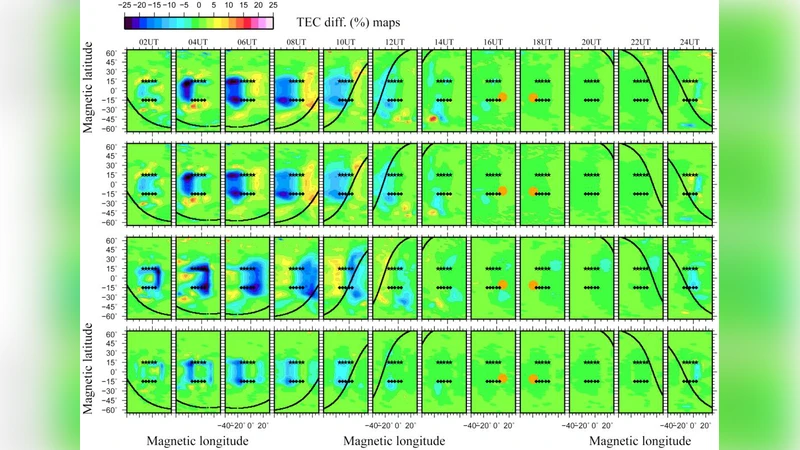
Simulation results reveal a clear and robust response of the ionospheric electron density to the imposed currents. When the current is directed upward (positive polarity), the model produces an enhancement of the electric field in the upper ionosphere, leading to an increase in electron concentration and a positive TEC perturbation that can reach up to 35 % above the background level. Conversely, a downward (negative) current generates a reduction of the electric field, depleting electrons and producing a negative TEC anomaly of comparable magnitude. The magnitude and sign of the TEC response are strongly modulated by the return‑current configuration. The “border” return current, which creates a compact circuit, yields the strongest electric fields and therefore the largest TEC deviations. A globally spread return current weakens the field and reduces the TEC perturbation, while the case without any return current produces the smallest effect because the circuit is incomplete and the field cannot fully develop.

Latitude also influences the outcome. At low latitudes, where background ionospheric conductivity is relatively low, the imposed currents generate larger electric fields and consequently larger TEC changes. At mid‑ and high‑latitudes, higher ambient conductivity partially shields the ionosphere, but the model still predicts TEC variations of 20 % or more, consistent with many observational reports. The spatial pattern of the simulated TEC anomalies—elongated along the meridional direction and extending over several thousand kilometers—matches the morphology of GPS‑derived pre‑seismic TEC disturbances documented in previous studies.

By reproducing both the amplitude (up to 35 %) and the spatial scale of observed TEC anomalies, the study provides quantitative support for the vertical‑current coupling hypothesis. It demonstrates that a relatively modest current density, when applied over a realistic geographic extent, is sufficient to drive ionospheric electric fields capable of producing the observed pre‑earthquake signatures. Moreover, the sensitivity of the TEC response to current direction and return‑current topology offers a potential diagnostic tool for distinguishing between different seismo‑ionospheric coupling mechanisms in future observational campaigns.

The authors acknowledge several limitations. The origin of the vertical currents is prescribed rather than derived from a physical model of stress‑induced charge separation, radon release, or other geophysical processes. The temporal evolution of the currents (duration, intermittency) is not explored, even though real pre‑seismic signals may be transient. Additionally, the model’s treatment of atmospheric chemistry and conductivity is simplified, and the impact of concurrent atmospheric disturbances (e.g., gravity waves, atmospheric tides) is not examined.

Future work is suggested in three main directions: (1) developing a physics‑based source model that links crustal stress, gas emission, and charge generation to the vertical current density; (2) integrating multi‑satellite (e.g., Swarm, COSMIC) and ground‑based GNSS observations to validate the simulated electric fields and TEC patterns in real time; and (3) extending the UAM framework to higher spatial resolution and coupling it with full‑wave atmospheric models to capture the interaction between electric currents, neutral dynamics, and ionospheric plasma. Successful implementation of these steps could pave the way for operational ionospheric monitoring systems that flag significant TEC anomalies as potential earthquake precursors, thereby contributing to the long‑standing goal of reliable seismic early warning.