Kernels for Vector-Valued Functions: a Review

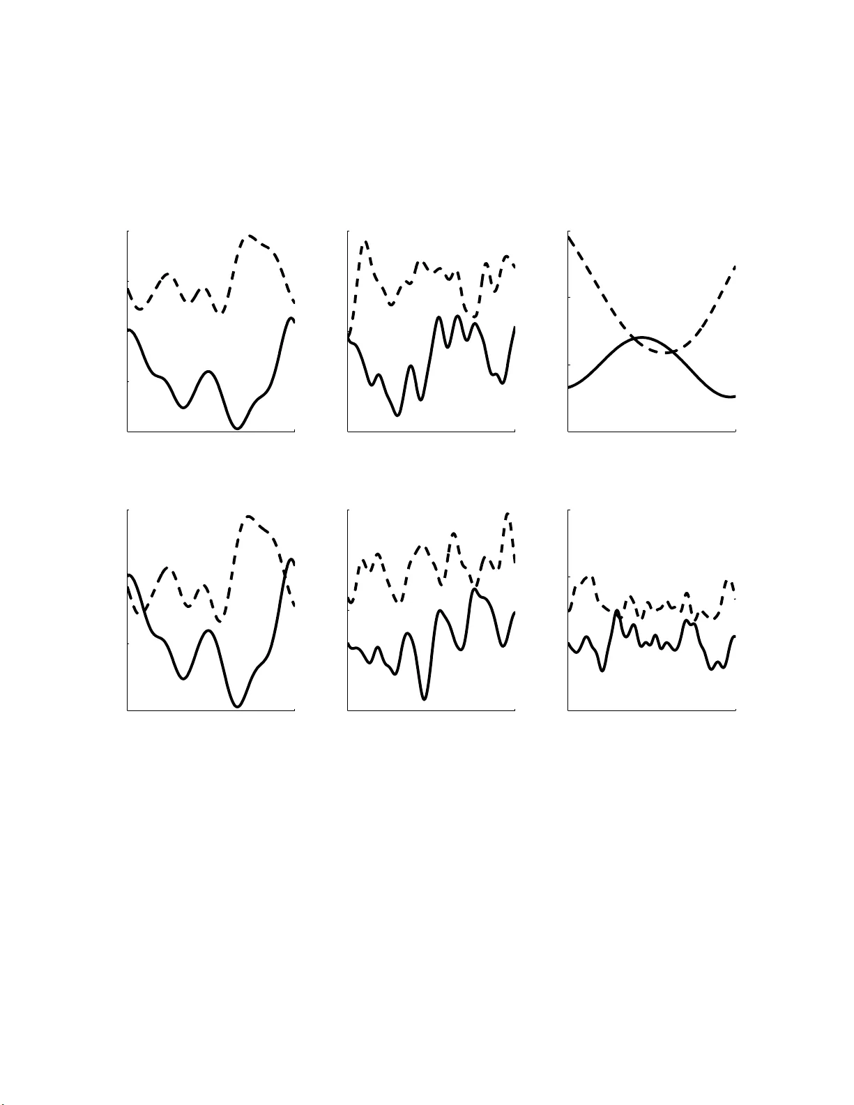
Kernels for V ector -V alued Functions: a Review Mauricio A. ´ Alvarez + , Lor enzo Rosasco ♯, † , Neil D. Lawr ence ⋆, ⋄ , ‡ - School of Computer Science, Uni versity of Manchester Manchester , UK, M 13 9PL. + Department of Electrical Engineering, Universidad T ecnol ´ ogica de Pereira, Colombia, 660003 ♯ - CBC L , McGovern Institut e, Massachusetts Institute of T echnolog y , Cambridge, MA, USA † -IIT@MIT Lab, Ist i tuto Italiano di T ecnologia, Genova, Italy ⋆ - Department of Computer Science, University of Shefﬁeld, UK ⋄ The S hefﬁeld Institute for T ranslational Neuroscience, Shefﬁeld, UK. malvarez@utp. edu.co, lrosasco@mit.edu, n.lawrence@sheffield. ac.uk November 26, 2024 Abstract Kernel methods are among t he most popular techniques in machine learning. From a regularization perspec- tive they play a central role in regularization th eory as they provide a natural choice for the hypotheses space and the regularization functiona l through the notion of reproducing kernel Hil ber t s paces. F rom a probabilistic per- spective they are the key in the context of Gaussian processes, where the kernel function is known as the covariance function. T raditionally , ker nel methods ha ve been used in supervised lear ning problem with scalar outputs and indeed there has been a considerable amount of wor k devoted to des igning and learning k e rnels. More recently there has been an increasing interest in methods that deal with multiple outputs, motivated partly by fr ameworks like multita sk learning. In this paper , we review different methods to des ign or learn valid k ernel funct ions for multiple outputs, pay i ng particular attention to the connection between probabilistic and functional methods. 1 Contents 1 Introduction 3 2 Learning Scalar Outpu ts with Kernel Method s 3 2.1 A Regulari zation Perspective . . . . . . . . . . . . . . . . . . . . . . . . . . . . . . . . . . . . . . . . . 4 2.2 A Bayesi an Perspective . . . . . . . . . . . . . . . . . . . . . . . . . . . . . . . . . . . . . . . . . . . . 5 2.3 A Connection B etween Bayesian and Reg ularization Point of V iews . . . . . . . . . . . . . . . . . . . 5 3 Learning Multip le Outputs with Kernels Metho ds 7 3.1 Multi-output Learning . . . . . . . . . . . . . . . . . . . . . . . . . . . . . . . . . . . . . . . . . . . . 7 3.2 Reproducing Kernel for V ector V alued Function . . . . . . . . . . . . . . . . . . . . . . . . . . . . . . 8 3.3 Gaussian Processes for V ector V alued Functions . . . . . . . . . . . . . . . . . . . . . . . . . . . . . . 9 4 Separable Kernels and Sum of Separable Kernels 10 4.1 Kernels and Reg ul arizers . . . . . . . . . . . . . . . . . . . . . . . . . . . . . . . . . . . . . . . . . . . 10 4.2 Coregionalization Models . . . . . . . . . . . . . . . . . . . . . . . . . . . . . . . . . . . . . . . . . . . 12 4.2.1 The Linear Mod el of Coregionalization . . . . . . . . . . . . . . . . . . . . . . . . . . . . . . . 12 4.2.2 Intrinsic Coregionalization Model . . . . . . . . . . . . . . . . . . . . . . . . . . . . . . . . . . 13 4.2.3 Comparison Between ICM and LMC . . . . . . . . . . . . . . . . . . . . . . . . . . . . . . . . 13 4.2.4 Linear Model of Coregionalization in Machine Learning and Statistics . . . . . . . . . . . . . 15 4.3 Extensions . . . . . . . . . . . . . . . . . . . . . . . . . . . . . . . . . . . . . . . . . . . . . . . . . . . 19 4.3.1 Extensions W ithin the Regularization Framewor k . . . . . . . . . . . . . . . . . . . . . . . . . 19 4.3.2 Extensions from the Gaussian Processe s Perspective . . . . . . . . . . . . . . . . . . . . . . . 20 5 Beyond Separable Kernels 20 5.1 Invariant Kernels . . . . . . . . . . . . . . . . . . . . . . . . . . . . . . . . . . . . . . . . . . . . . . . 20 5.2 Further Extensions of the LMC . . . . . . . . . . . . . . . . . . . . . . . . . . . . . . . . . . . . . . . . 21 5.3 Process Convolutions . . . . . . . . . . . . . . . . . . . . . . . . . . . . . . . . . . . . . . . . . . . . . 22 5.3.1 Comparison Between Process Convolutions and LMC . . . . . . . . . . . . . . . . . . . . . . 23 5.3.2 Other Approaches Related to Process Convolutions . . . . . . . . . . . . . . . . . . . . . . . . 23 6 Inference and Co mputational Considerations 26 6.1 Estimation of Parameters i n Regularization Theor y . . . . . . . . . . . . . . . . . . . . . . . . . . . . 26 6.2 Parameters Estimation for Gaussian Processes . . . . . . . . . . . . . . . . . . . . . . . . . . . . . . . 27 7 Applications of Mu ltivariate Kernels 29 8 Discussion 30 2 1 Introduction Many mo dern applications of mach ine learning require sol ving sever al decision making or pr ediction problems and exploiting dependencies between the problems is often the k ey to obtain better results and coping with a lack of data (to s o lve a problem we can b orrow strength from a distinct but related problem). In sensor networks , f or example, mi ssing signals from certain sensors may be predicted by exploiting their cor- relation with observed signals acquired from other sensors [72]. In geostatistics , predicting the concentration of heavy pollutant metals, which ar e e xpensive to measure, can be done usi ng inexpensive and over sampled vari- ables as a proxy [37]. In computer graphics , a common theme is the animation and s imulation of physically plausible humanoid motion. Given a set of poses that delineate a particular moveme nt (for example , walki ng), we are faced with the task of completing a s equence by ﬁlling in the mi s sing frames with na tural-looking poses. Human move- ment exhibits a high-de g ree of cor relation. Consider , for example, the way we w alk. When mo ving t he right leg forward, we un consciously pr epare the left leg, which is curren tly touching the ground, to s tart moving as soon as the ri ght leg reaches the ﬂoor . At the same time, our hands move synchronously with our leg s. W e can explo i t these implicit correlations for predicting new poses and for generating new natural-looking walking sequences [106]. In text categ orization , one document can be assigned to multiple topics or have multiple labels [50]. In all the examples above, the simplest approach i gnores the potential correlation among the different output compo- nents of the problem and employ models that make predictions individ ually for each output. However , these examples suggest a different approach through a joint prediction exploiting the interaction between the different components to improve on individual predictions. W ithin the machine learning community this type of model ing is often broadly referred to to as multitask learning . Again the key idea is that information shared between different tasks can lead to improved performance in comparison to learning th e same tasks individually . These ideas are related to tran sfer learning [97, 20, 12, 74], a term which refers to systems that l e arn by transferring knowledge between different domains, for example: “wh at can we learn about running through see ing walking?” More formally , th e classical supervised learning problem requires estimating the output for any given input x ∗ ; an estimator f ∗ ( x ∗ ) is built on the basis of a training set consisting of N input-output pairs S = ( X , Y ) = ( x 1 , y 1 ) , . . . , ( x N , y N ) . The input space X is us ually a space of vectors, while the output s p ace is a space of scalars . In multiple output learning ( M OL) the output space is a space of vectors ; the estimator is now a vector valued function f . Indeed, this situation can also be described as the problem of solving D di s tinct cl ass ical supervised problems, where each problem is descr ibed by one of the components f 1 , . . . , f D of f . As mentioned before, the key idea is to work under the assumption th at the problems are in some wa y related. The idea is then to exploit the relation among the p roblems to improve upon solving each problem separately . The goal of this survey is twofold. First, we aim at di scussing recent results in multi-output/multi-task learning based on kernel methods and Gaussian processes providing an account of the state of the art in the ﬁeld. Second, we analyze systematically the connections between Bayesian and regularization (frequentist) approaches. Indeed , related techniques have been propos ed from different perspectives and drawing clearer connections can boost advances in the ﬁeld, while fostering col laborations between different communities. The plan of the paper follows. In chapter 2 we give a brief review of the main ideas underlying kernel methods for s calar learning, introducing the concepts of regularization in reproducing ker nel Hilbert spaces and Gaussian processes. In chapt er 3 we describe how similar concepts extend to the context of vector valued functions and discuss different settings that can be conside red. In chapters 4 and 5 we discuss approaches to constructing mul- tiple output kernels, drawing conn ections between the Baye sian and r egularization framewor k s. The parameter estimation problem and the computationa l complexity problem are both described i n chapter 6 . In chapter 7 we discuss some potential applications th at can be see n as multi-output learning. Fi nally we con clude in chapter 8 with some remark s and discussion. 2 Learning Scalar O utputs with Kernel Methods T o make the paper sel f contained, we will start o ur study reviewing the classical problem of learning a scalar valued function, se e for example [100, 40, 10, 82]. This will also serve as an opportunity to review conn ections between Bayes ian and regularization methods. As we mentioned above, in the classical s etting o f supervised learning, we have to build an es timator (e.g . a classiﬁcation r ule or a regression function) on th e basis of a training set S = ( X , Y ) = ( x 1 , y 1 ) , . . . , ( x N , y N ) . Given a symmetric and positive bivariate function k ( · , · ) , namely a kernel , one of t he mo s t po p ular estimators in machine learning is deﬁned as f ∗ ( x ∗ ) = k ⊤ x ∗ ( k ( X , X ) + λN I ) − 1 Y , (1) 3 where k ( X , X ) has entries k ( x i , x j ) , Y = [ y 1 , . . . , y N ] ⊤ and k x ∗ = [ k ( x 1 , x ∗ ) , . . . , k ( x N , x ∗ )] ⊤ , where x ∗ is a new input point. Int erestingly , such an estimator can be d erived from two different, though, related perspectives. 2.1 A Regularization Perspective W e wil l ﬁrst describe a regularization (frequentist) pe rspective (see [35, 105, 100, 86]). The key point in this setting is that the function of interest is assumed to belong to a reproducing kernel Hilbert space (RKHS), f ∗ ∈ H k . Then the e s timator is derived as the minimizer of a regul ar ized functional 1 N N X i =1 ( f ( x i ) − y i ) 2 + λ k f k 2 k . (2) The ﬁrst ter m in the functional is the so called emp i rical risk and it is the sum of the squared errors. It is a measure of the pr ice we pay when predicting f ( x ) in place of y . The second term in t he functional is the (squared) norm in a RKHS. This latter concept plays a key role, so we review a few essential concepts (see [87, 6, 105, 25]). A RKHS H k is a Hilbert space o f functions and can be deﬁned by a reproducing k ernel 1 k : X × X → R , which is a symme tr ic, positive deﬁnite function. The latter assumption amounts to requir ing the matrix with entries k ( x i , x j ) to be positive for any (ﬁnit e) sequence ( x i ) . Given a k ernel k , the RKHS H k is the Hilbert space such that the function k ( x , · ) belongs to belongs to H k for all x ∈ X and f ( x ) = h f , k ( x , · ) i k , ∀ f ∈ H k , where h· , ·i k is the inner product in H k . The l atter property , known as the reproducing property , gives the n ame to the space. T wo further properties make RKHS appeali ng: • functions in a RKHS are in the closure of the linear combinations of the kernel at given points, f ( x ) = P i k ( x i , x ) c i . This allows us to d escribe, i n a uniﬁed framework, linear models as well as a variety of generalized linear models ; • the norm in a RKHS can be wri tten as P i,j k ( x i , x j ) c i c j and is a nat ural measure of how complex i s a function. Speciﬁc examples are given by the shrinkag e point of view taken in r idge regression with linear models [40] or the regularity expressed in terms of magnitude of derivatives, as is done in spl ine models [105]. In this setting the functional (2 ) can be de rived either from a regularization point of view [35, 105] or from the theory of empirical ris k minimization (ERM) [100]. In the former , one observes that, if the s pace H k is large enough, the minimi zation of the empirical error is ill-pos ed, and in particular i t responds in a n unstable manner to noise, or when the number of samples is low Adding the squared norm stabilizes the problem. The latter point of view , starts from the analysis of ERM showing that generalization to new sample s can be achieved if there is a tradeoff between ﬁtting and complexity 2 of the estimator . The functional (2) can be s e en as an instance of such a trade-off. The explicit form of th e estimator is derived i n two steps. Fir st, one can show that the minimizer of (2) can always be written as a linear combination of the kernels centered at the training set points, f ∗ ( x ∗ ) = N X i =1 k ( x ∗ , x i ) c i = k ⊤ x ∗ c , see for example [65, 19]. The above result is the well known representer theorem originally proved in [51] (see also [88] and [26] fo r recent results and further references). The explicit for m of the coef ﬁcients c = [ c 1 , . . . , c N ] ⊤ can be then d erived by substituting for f ∗ ( x ∗ ) in (2). 1 In the following we will simply write kernel rather than reproducing kernel. 2 For example, a measure of complexity is the V apnik–Chervonenkis dimension [86] 4 2.2 A Bayesian Perspective A Gaussian process (GP) is a stochastic process with the i mportant charact eristic that an y ﬁnite number of random variables, taken from a realization of the GP , follows a joint Gaussian distri bution. A GP is usually used as a prior distribution for functions [82 ]. If th e function f follo ws a Gaussian process we wr i te f ∼ G P ( m, k ) , where m is the mean function and k the covariance or kernel function. The mean function and the covariance function completely specify the Gaussian process . In other words the above assumption means that for any ﬁnite set X = { x n } N n =1 if we let f ( X ) = [ f ( x 1 ) , . . . , f ( x N )] ⊤ then f ( X ) ∼ N ( m ( X ) , k ( X , X )) , where m ( X ) = [ m ( x 1 ) , . . . , m ( x N )] ⊤ and k ( X , X ) is the ker nel matrix. In the following, unles s otherwise stated, we assume that the mean vector is zero. From a Bayesian point of view , the Gaussian process speciﬁes our prior beliefs about the properties of the func- tion we are model i ng. Our beliefs are updated i n the presence of data by me ans of a likelihood fu n ction , that relates our prior assumptions to the actua l obser vations. This le ads to an updated distr i bution, the posterior distrib u tion , that can be used, for example, fo r predicting test cases. In a regression context, the likelihood function is usually Gaussian and expresses a linear relation between the observations and a given model for the data that is cor rupted with a zero mean Gaussian noise , p ( y | f , x , σ 2 ) = N ( f ( x ) , σ 2 ) , where σ 2 corresponds to th e variance of the noise. Noise is assumed to be independent an d i dentically distri buted. In this wa y , the likelihood funct ion factorizes over d ata points, given the set of inputs X an d σ 2 . The posterior distribution can be computed analytically . For a test input vector x ∗ , gi ven the training data S = { X , Y } , this posterior distri bution is given by , p ( f ( x ∗ ) | S , x ∗ , φ ) = N ( f ∗ ( x ∗ ) , k ∗ ( x ∗ , x ∗ )) , where φ denotes the set of parameters wh ich include the va riance of the nois e , σ 2 , and any parameters from the covariance function k ( x , x ′ ) . Here we have f ∗ ( x ∗ ) = k ⊤ x ∗ ( k ( X , X ) + σ 2 I ) − 1 Y , k ∗ ( x ∗ , x ∗ ) = k ( x ∗ , x ∗ ) − k ⊤ x ∗ ( k ( X , X ) + σ 2 I ) − 1 k x ∗ and ﬁn ally we note th at if we are interested into the distribution of th e noisy predictions, p ( y ( x ∗ ) | S , x ∗ , φ ) , it is easy to se e that we simply have to add σ 2 to the exp ress ion for the predictive variance (see [82]). Figure 1 repr esents a posteri or predictive distri bution for a data vector Y with N = 4 . Data p oints are repre- sented as dots in the ﬁgure. The solid line represents the mean function predicted, f ∗ ( x ∗ ) , while th e shaded region corresponds to two standard deviations away from the mean. This shaded reg ion is speciﬁed using the predicted covariance function, k ∗ ( x ∗ , x ∗ ) . Notice how the uncertainty in the prediction increases as we move awa y from the data points. Equations for f ∗ ( x ∗ ) and k ∗ ( x ∗ , x ∗ ) are obtained under the assumption of a Gaussian likelihood, common in regression setups. For non-Gaussian li kelihoods, for example i n classiﬁcation problems, closed f o rm solutions are not longer possible. In this case, one can resor t to d ifferent appr oximations, including the L aplace approximation and variational me thods [82]. 2.3 A Connection Between Bayesian and Regularization Point of V iews Connections between regulari zation theory and Gaussian process prediction or Bayes ian models for prediction have been pointed out elsewhere [78, 105, 82]. Here we just give a very brief sketch of the argument. W e restrict ourselves to ﬁnite dime nsi o nal RKHS. Under this assumption one can show that every RKHS can be described in terms of a fe ature map [100], that is a map Φ : X → R p , such that k ( x , x ′ ) = p X j =1 Φ j ( x )Φ j ( x ′ ) . 5 −0.2 0 0.2 0.4 0.6 0.8 1 1.2 −2.5 −2 −1.5 −1 −0.5 0 0.5 1 1.5 2 x f ( x ) Figure 1: E xample of a p redictive posterior distribution inferred with N = 4 . The solid line corresponds to the predictive mea n, the shaded region corresponds to two standard deviations of the prediction. Dots are values of the output function Y . W e have also included some samples f rom the posterior distribution, shown as dashed lines. In fact in this case one can show that functions in the RKHS with ker nel k can be written as f w ( x ) = p X j =1 w j Φ j ( x ) = h w , Φ( x ) i , an d k f w k k = k w k . Then we can build a Gaussian p rocess by assuming th e coefﬁcient w = w 1 , . . . , w p to be distributed according to a multivariate Gaussian di s tribution. Roughly speaking, in this case the assumption f ∗ ∼ G P (0 , k ) becomes w ∼ N (0 , I p ) ∝ e −k w k 2 . As we noted before i f we assume a Gaussian likelihood we have P ( Y | X , f ) = N ( f ( X ) , σ 2 I D ) ∝ e − 1 σ 2 k f w ( X ) − Y k 2 n , where f w ( X ) = ( h w , Φ( x 1 ) i , . . . , h w , Φ( x n ) i ) and k f w ( X ) − Y k 2 n = P n i =1 ( h w , Φ( x i ) i − y i ) 2 . Then the po sterior distribution is proportional to e − ( 1 σ 2 k f w ( X ) − Y k 2 n + k w k 2 ) , and we se e that a maximum a posterio r i estimate will in t urn g ive the minimization prob lem deﬁning T ikhonov regularization [98], where the regularization parameter is now related to the noise variance. 6 W e note that in regularization the squared error i s often replaced by a mo re general error term 1 N P N i =1 ℓ ( f ( x i ) , y i ) . In a regular ization perspe ctive, the loss function ℓ : R × R → R + measure the error we incur when predicting f ( x ) in place of y . The choice of the loss funct ion is problem dependent . Often us ed examples are the square loss, the logistic loss or the hinge loss us e d in support vector machines (see [86]). The choice o f a l o ss function in a regularization setting can be contrasted to th e choice of the likel ihood in a Bayesian setting. In this context, the likelihood function model s how the observations d e viate from the ass umed true model in th e generative process. The notion of a los s function is philosop hically different. It represents the cost we pay for making errors. In Bayes ian model ing decisio n making is separated from inference. In the inference stage the pos terior distributions are computed evaluating the uncertainty in the mod e l. The loss function appears only at the second stage of the analysis, known as the decision stage, and weighs how incorrect decisions are penalized given the current un certainty . However , whilst the t wo notions are philosophically very different, we can s ee that, due to the formulation of the fr ameworks, the l oss function and the log likelihood provide the same role mathema tically . The di scussion in the previous sections shows that the notion of a ke r nel plays a crucial role in statistical modeling both in the Bay esian perspective (as the covariance function of a GP) and the regularization per spective (as a reproducing k ernel). Indeed , for scalar valued problems there is a rich literature on the design of kernels (see for ex ample [86, 90, 82] and references therein). In the next sections we show how the concept of a kernel can be used i n multi-output learning problems . Before doing that, we describe how the concepts o f RKHSs and GPs translate to the s e tting of vector valued learning. 3 Learning Multiple Outputs with Kernels Me thods In this chapter we discuss the basic setting for learning vector valued functions and related problems (multiclass , multilabel) and then d escribe how th e concept of kernels (reproducing kernels and covariance fun ction for GP) translate to this setting. 3.1 Multi-output Learning The problem we are interested in is that of learning an unknown funct ional relationship f between an input space X , for example X = R p , an d an output space R D . In th e following we will s ee that the problem can be tac kled either assuming that f belongs to reproducing k ernel Hilber t s p ace of vector valued functions or ass uming that f is drawn from a vector valued Gaussian process. Before doing this we describe s e veral related settings all falling under the framework of multi-output learning. The natural extension of the traditional (scalar) supervis e d learning problem i s the one we d i scussed in the introduction, when the data are pairs S = ( X , Y ) = ( x 1 , y 1 ) , . . . , ( x N , y N ) . For example this is the typical se tting for problems such as motion/velocity ﬁelds estimation. A special case is that of multi-category classi ﬁcation problem or multi-label problems, where if we have D classes each input point can be asso ci ated to a (binary) coding vector where, for example 1 stands fo r presence ( 0 for absence) of a class instance.The simplest example is the so called one vs all approach to multiclass classiﬁcation which, if we have { 1 , . . . , D } classes, amoun ts t o t he coding i → e i , where ( e i ) is the canonica l basis of R D . A more general situation is that wher e different outputs might have d ifferent training set cardinalities, different input points or in the extreme case even different input spaces. More formally , in this case we have a training set S d = ( X d , Y d ) = ( x d, 1 , y d, 1 ) , . . . , ( x d,N d , y d,N d ) for each component f d , with d = 1 , . . . , D , where the number of data associated with each output, ( N d ) might be d i fferent and th e input for a compo nent might belong to different input space ( X d ) . The terminology used in machine learning often does not distinguish the different settings above and the term multitask learning is often used. In this paper we use the term multi-output lear ning or vector valued learning to deﬁne the general class of problems and use the term multi-task for the case where each component has different inputs. Indeed in this very general situation each compo nent can be thought of as a dis tinct task possibly related to other tasks (components). In the geostatistics literature, if each output has the same set of inputs the model is called isotopic and heterotopic i f each output to be associated with a different set of inputs [ 104] . Heter otopic data is further classi ﬁe d into entirely hetero topic data , where the variables have no sample locations in common, and partially heter otopic data , wh ere the variables shar e some s ample locations. In mach ine learning, the partially heterotopic case is sometimes referred to as asymmetric mu ltitask learning [112, 21]. The notation in the mul titask l earning scenario (heterotopic case) is a bit more involved. T o simplify the nota- tion we ass ume that the number o f data for each output is the same. Moreover , for the sake of simp l icity sometimes 7 we restrict the presentation to the isotopic setting, though the models can usually readily be extended to the mo re general setting. W e will use the notation X to indicate the collection of all the training input po ints, { X j } N j =1 , and S to d enote the colle ction of all t he training data. Also we will use the n otation f ( X ) to indicate a vector valued function evaluated at d i fferent training points. This notation has slig htly different meaning depending on the way the input points are sample d. If th e input to all the components are the same then X = x 1 , . . . , x N and f ( X ) = f 1 ( x 1 ) , . . . , f D ( x N ) . If the input for the different components are different then X = { X d } D d =1 = X 1 , . . . , X D , where X d = { x d,n } N n =1 and f ( X ) = ( f 1 ( x 1 , 1 ) , . . . , f 1 ( x 1 ,N )) , . . . , ( f D ( x D , 1 ) , . . . , f D ( x D ,N )) . 3.2 Reproducing Kernel for V ecto r V a lue d Function The deﬁnition of RKHS for vector valued functions parallels the one in the scalar , with the main difference that the reproducing kernel is now matrix valued , see for example [ 65, 19] . A reproducing kernel is a symmetric function K : X × X → R D × D , such that for any x , x ′ K ( x , x ′ ) is a positive sem i -deﬁnite matrix . A vector valued RKHS i s a Hilbert space H of functions f : X → R D , such that for very c ∈ R D , and x ∈ X , K ( x , x ′ ) c , as a function of x ′ belongs to H and moreover K has the reproducing property h f , K ( · , x ) c i K = f ( x ) ⊤ c , where h· , ·i K is the inner product in H . Again, the choice of the kernel corresponds to the choice of the representation (parameterization) for the func- tion of interest. In fact any function in the RKHS is in the closure of the set of linear combinations f ( x ) = p X i =1 K ( x i , x ) c j , c j ∈ R D , where we n ote tha t in the above equation each term K ( x i , x ) is a matrix acting o n a vector c j . The norm in the RKHS typically p rovid es a measure of the complexity of a function and this will be the subject of the next sections. Note that the deﬁnition of vector valued RKHS can be described in a component-wise fashion i n the following sense. T he kernel K can be described by a scalar kernel R acting joint ly on input examples and task indices, that is ( K ( x , x ′ )) d,d ′ = R (( x , d ) , ( x ′ , d ′ )) , (3) where R is a scalar reproducing k ernel on the s pace X × { 1 , . . . , D } . This latter point of view is use ful while dealing with mul titask learning, see [28] for a discussion. Provided with the above concepts we can follow a regularization approach to deﬁne an estimator by mi nimiz- ing the regul ar i zed e mp i rical error (2), which in this case can be written as D X j =1 1 N N X i =1 ( f j ( x i ) − y j,i ) 2 + λ k f k 2 K , (4) where f = ( f 1 , . . . , f D ) . Once again the solution i s given by the representer theorem [65] f ( x ) = N X i =1 K ( x i , x ) c i , and the coefﬁcient satisﬁes the linear system c = ( K ( X , X ) + λ N I ) − 1 y , (5) where c , y are N D vectors obtained concat enating the coefﬁcients and the output vectors , and K ( X , X ) i s an N D × N D with entries ( K ( x i , x j )) d,d ′ , for i, j = 1 , . . . , N and d, d ′ = 1 , . . . , D (see for e xample [65]). More explicitly K ( X , X ) =      ( K ( X 1 , X 1 )) 1 , 1 · · · ( K ( X 1 , X D )) 1 ,D ( K ( X 2 , X 1 )) 2 , 1 · · · ( K ( X 2 , X D )) 2 ,D . . . · · · . . . ( K ( X D , X 1 )) D , 1 · · · ( K ( X D , X D )) D ,D      (6) 8 where each blo ck ( K ( X i , X j )) i,j is an N by N matrix (here we make the simpl i fying assumption that e ach output has same number of training data). Note that given a new point x ∗ the correspo nding predi ction is given by f ( x ∗ ) = K ⊤ x ∗ c , where K x ∗ ∈ R D × N D has entries ( K ( x ∗ , x j )) d,d ′ for j = 1 , . . . , N and d, d ′ = 1 , . . . , D . 3.3 Gaussian Processes for V ector V alued Functio ns Gaussian process methods for modeling vector-valued functions follow the same approach as in the single o utput case. Recall that a Gaussi an process is deﬁned as a collection o f random va riables, such that any ﬁnite number of them follows a joint Gaussian distribution. In the single output case, the random variables are associated to a si ngle process f evaluated at different values of x w hile in the multiple output case, the random variables are associated to different processes { f d } D d =1 , evaluated at different values of x [24, 37, 102]. The vector-valued function f is assumed to fo llow a Gaussian process f ∼ G P ( m , K ) , (7) where m ∈ R D is a vector which compo nents are the mean functions { m d ( x ) } D d =1 of each output and K is a positive matrix valued function as in section 3.2. The entries ( K ( x , x ′ )) d,d ′ in the matrix K ( x , x ′ ) correspond to the covariances between the outputs f d ( x ) and f d ′ ( x ′ ) and express the degree of correlation or similarity between them. For a s et of inputs X , the prior distri bution over the vector f ( X ) i s given by f ( X ) ∼ N ( m ( X ) , K ( X , X )) , where m ( X ) is a vector tha t concatena tes the mean vectors associated t o th e outputs and the covariance matrix K ( X , X ) i s the block partitioned matrix in (6). W ithout loss of generality , we assume the mean vector to be zero. In a regression context, the likelihood function for the outputs is often taken to be Gaussian distribution, so that p ( y | f , x , Σ) = N ( f ( x ) , Σ) , where Σ ∈ R D × D is a diago nal matrix with elements 3 { σ 2 d } D d =1 . For a Gauss ian likelihood, the predictive distribution and the marginal likeli hood can be derived analytically . The predictive distribution for a new vector x ∗ is [82] p ( f ( x ∗ ) | S , f , x ∗ , φ ) = N ( f ∗ ( x ∗ ) , K ∗ ( x ∗ , x ∗ )) , (8) with f ∗ ( x ∗ ) = K ⊤ x ∗ ( K ( X , X ) + Σ ) − 1 y , K ∗ ( x ∗ , x ∗ ) = K ( x ∗ , x ∗ ) − K x ∗ ( K ( X , X ) + Σ ) − 1 K ⊤ x ∗ , where Σ = Σ ⊗ I N , K x ∗ ∈ R D × N D has entries ( K ( x ∗ , x j )) d,d ′ for j = 1 , . . . , N and d, d ′ = 1 , . . . , D , and φ denotes a possible set o f hyperparameters of the covariance fun ction K ( x , x ′ ) used to compute K ( X , X ) and the variances of the noise for each output { σ 2 d } D d =1 . Again we note that if we are interested i nto the distribution of the noisy predictions it is easy to see that we simply have to add P Σ to the ex pression of the prediction variance. The above expression fo r the mean prediction coincides again with t he prediction of the es timator d erived in the regularization framework. In the following chapters we describe s e veral possi ble choices of k ernels (covariance function) for multi-output problems. W e start in the next cha pter wit h k e rnel functions that clearly separate t he contributions of input and output. W e wil l see later alternative ways to construct kernel functions that interleave both contributions in a non trivial way . 3 This relation d erives fr om y d ( x ) = f d ( x ) + ǫ d ( x ) , for each d , wher e { ǫ d ( x ) } D d =1 are ind ependent white Gaussian noise processes with variance σ 2 d . 9 4 Separable Kernels and Sum of Separable Ker nels In this chapter we review a special class of multi-output ke rnel functions that can be formulated as a sum of products between a ker nel function for the input space alone, and a ker nel function that encodes the interactions among the outputs. W e refer to this type of multi-output kernel functions as sep arable kernels and sum of separable kernels (SoS ker nels). W e consid er a class o f ker nels of the form ( K ( x , x ′ )) d,d ′ = k ( x , x ′ ) k T ( d, d ′ ) , where k, k T are scalar kernels on X × X and { 1 , . . . , D } × { 1 , . . . , D } . Equivalently one can consider the matrix ex pression K ( x , x ′ ) = k ( x , x ′ ) B , (9) where B is a D × D symmetr i c and pos itive semi-deﬁnite matrix. W e call this class of kernels separable since, comparing to (3), we see that the contribution of input and output is decoupled. In the s ame spirit a more general class of kernels is gi ven by K ( x , x ′ ) = Q X q =1 k q ( x , x ′ ) B q . For this class of kernels, the ker nel matrix associated to a data set X has a simple r form and can be wr itten as K ( X , X ) = Q X q =1 B q ⊗ k q ( X , X ) , (10) where ⊗ represents the Kronecker product between matrices. W e call this class of kernels sum of separable ker nels (SoS ker nels ). The simple st example of separ able k ernel is given by setting k T ( d, d ′ ) = δ d,d ′ , where δ d,d ′ is the Kronecker delta. In this case B = I N , that is all the outputs are tr eated as being un related. In this case the kernel matrix K ( X , X ) , associated to some se t of data X , becomes block diagonal. Since the of f diagonal terms en code output relatedness. W e can see that the matrix B encodes dependencies among the outputs. The key question is how to choose the scalar kernels { k q } Q q =1 and especially how to desig n, or le arn, the matri- ces { B q } Q q =1 . This is the subject we discuss in the next few sections. W e will see that one can approach the problem from a regularization po int of view , where ker nels will be deﬁned by the choice of suitable regularizers, o r , from a Bayesian point of view , constructing covariance functions from expli cit generative models for the different output components. As it turns out these two points of view are equivalent and allo w for two different interpretations of the same class of models. 4.1 Kernels and Regularizers In this section we largely follow the results in [64, 65, 27] and [7]. A poss i ble way to desi gn mul ti-output kernels of th e form ( 9) is given by the following result. If K is given by (9) then is pos sible to prove that the norm of a function in the corresponding RKHS can be written as k f k 2 K = D X d,d ′ =1 B † d,d ′ h f d , f d ′ i k , (11) where B † is the pseudoinverse of B and f = ( f 1 , . . . , f D ) . The above expression gives another way to see why the matrix B encodes the r elation among the components. In fact, we can interpret the right hand side in the above expression as a regularizer inducing speciﬁc coupling among different tasks h f t , f t ′ i k with different weights given by B † d,d ′ . This result says that any such regularizer induces a ke rnel of the for m ( 9). W e illustrate the above id ea with a fe w examples. 10 Mixed Effect Regu l arizer Consider the regularizer given by R ( f ) = A ω C ω D X ℓ =1 k f ℓ k 2 k + ω D D X ℓ =1 k f ℓ − 1 D D X q =1 f q k 2 k ! (12) where A ω = 1 2(1 − ω )(1 − ω + ω D ) and C ω = (2 − 2 ω + ω D ) . The above regularizer i s composed of two terms : the ﬁrst is a standard regularization term on the n orm of each component of the estimator; th e second forces each f ℓ to be clo se to the mean estimator across the components, f = 1 D P D q =1 f q . The corresponding kernel imposes a common similarity structur e between all th e output components and the strength of the similari ty is controlled by a parameter ω , K ω ( x , x ′ ) = k ( x , x ′ )( ω 1 + (1 − ω ) I D ) (13) where 1 is the D × D matrix whose entries are all e q ual to 1 , and k is a scalar kernel on the i nput s pace X . Setting ω = 0 corresponds to treatin g all compo nents independently and the possible similarity among them is not exploited . Conversely , ω = 1 is equivalent to assuming that all compo nents are identical an d are ex plained by the same function. By tuning the parameter ω the above k ernel interpolates between this two o pposites cases. W e note that from a Bayesian pers pective B is a correlation matrix with all the o ff-diago nals equal to ω , which means that the o utput of the Gaussian process are exchangeable. Cluster Based Regularizer . Another example of regularizer , proposed in [28], is based on the idea of grouping the components in to r clusters and enfor cing the components in each cluster to b e simi lar . Follo wing [47], l e t us deﬁne the matrix E as the D × r matrix, wh ere r is t he number of clusters , such tha t E ℓ,c = 1 i f the component l belongs to cluster c and 0 otherwise. Then we can comp ute the D × D matrix M = E ( E ⊤ E ) − 1 E ⊤ such that M ℓ,q = 1 m c if components l and q belong to the same cluster c , and m c is its cardinality , M ℓ,q = 0 otherwise. Furthermore let I ( c ) be the index set of the components that belong to cl us ter c . Then we can conside r the fol lowing regularizer that forces components belonging to the same cluster to be close to each other: R ( f ) = ǫ 1 r X c =1 X ℓ ∈ I ( c ) k f ℓ − f c k 2 k + ǫ 2 r X c =1 m c k f c k 2 k , (14) where f c is the mean of t he components in cluster c and ǫ 1 , ǫ 2 are parameters ba lancing the two terms . Straig ht- forward calculations show that the previous regularizer can be rewritten as R ( f ) = P ℓ,q G ℓ,q h f ℓ , f q i k , where G ℓ,q = ǫ 1 δ lq + ( ǫ 2 − ǫ 1 ) M ℓ,q . (15) Therefore the corresponding matrix valued kernel is K ( x , x ′ ) = k ( x , x ′ ) G † . Graph Regularizer . Following [64, 91], we can deﬁne a regularizer that, in addition to a sta ndard regulari za- tion on the single components, forces stronger or weaker similarity between them thr ough a given D × D positive weight matrix M , R ( f ) = 1 2 D X ℓ,q = 1 k f ℓ − f q k 2 k M ℓq + D X ℓ =1 k f ℓ k 2 k M ℓ,ℓ . (16) The regularizer J ( f ) can be rewritten as: D X ℓ,q = 1  k f ℓ k 2 k M ℓ,q − h f ℓ , f q i k M ℓ,q  + D X ℓ =1 k f ℓ k 2 k M ℓ,ℓ = D X ℓ =1 k f ℓ k 2 k D X q =1 (1 + δ ℓ,q ) M ℓ,q − D X ℓ,q = 1 h f ℓ , f q i k M ℓ,q = D X ℓ,q = 1 h f ℓ , f q i k L ℓ,q (17) where L = D − M , with D ℓ,q = δ ℓ,q  P D h =1 M ℓ,h + M ℓ,q  . Therefore th e resulting kernel will be K ( x , x ′ ) = k ( x , x ′ ) L † , with k ( x , x ′ ) a s calar kernel to be chosen according to the problem at hand. In the next section we will see how model s related to those described above can be derived from suitable generative models. 11 4.2 Coregionalization Models The use of probabilistic models and Gaussian processes for multi-output learning was pioneered and largely d e - veloped in the context of g eostatistics, where prediction over vector-valued output data is known as cokriging . Geostatistical approaches to multivariate mod elling are mostly formulated around the “linear model of coregi on- alization” (LMC) [49 , 37], t hat can be consi d ered as a gener ative approach for develop ing valid covariance fun c- tions. Covariance functions obt ained un der the LMC assumption follow the form of a sum of separable kernels. W e will start consid ering this model and then discuss how several model s recently proposed in the machine learn- ing literature are special cases of the LMC. 4.2.1 The Linear Model of Coregionaliza tion In the linear model of coregionalization, the outputs are ex pressed as li near combinations of independent random functions. This is done in a way that ensures that the resulting covariance function (e x pressed jointly over all the outputs and the i nputs) is a valid positive semideﬁnite function. Consider a s et of D outputs { f d ( x ) } D d =1 with x ∈ R p . In the LMC, each component f d is expressed as [49] f d ( x ) = Q X q =1 a d,q u q ( x ) , where the latent functions u q ( x ) , have mean zero and covari ance co v[ u q ( x ) , u q ′ ( x ′ )] = k q ( x , x ′ ) if q = q ′ , and a d,q are scalar coefﬁcients. The process es { u q ( x ) } Q q =1 are independent for q 6 = q ′ . The independence assumption can be relaxed and such relaxation is presented as an extension in section 4.3. Some of the basic proces s es u q ( x ) and u q ′ ( x ′ ) can have the same covariance k q ( x , x ′ ) , while remaining independent. A similar expression f o r { f d ( x ) } D d =1 can be wr itten grouping the functions u q ( x ) which share the same covari- ance [49, 37] f d ( x ) = Q X q =1 R q X i =1 a i d,q u i q ( x ) , (18) where the functions u i q ( x ) , with q = 1 , . . . , Q and i = 1 , . . . , R q , have mean equal to zero and covariance co v[ u i q ( x ) , u i ′ q ′ ( x ′ )] = k q ( x , x ′ ) if i = i ′ and q = q ′ . Express ion (18) means that t here ar e Q g roups o f fun ctions u i q ( x ) and that the functions u i q ( x ) within each group share the same covariance, b ut are independent. The cr oss covariance between any two functions f d ( x ) and f d ′ ( x ) is gi ven in terms of the covariance functions fo r u i q ( x ) co v[ f d ( x ) , f d ′ ( x ′ )] = Q X q =1 Q X q ′ =1 R q X i =1 R q X i ′ =1 a i d,q a i ′ d ′ ,q ′ co v[ u i q ( x ) , u i ′ q ′ ( x ′ )] . The covariance co v[ f d ( x ) , f d ′ ( x ′ )] is given by ( K ( x , x ′ )) d,d ′ . Due to the independence of the functions u i q ( x ) , the above expressio n reduces to ( K ( x , x ′ )) d,d ′ = Q X q =1 R q X i =1 a i d,q a i d ′ ,q k q ( x , x ′ ) = Q X q =1 b q d,d ′ k q ( x , x ′ ) , (19) with b q d,d ′ = P R q i =1 a i d,q a i d ′ ,q . The kernel K ( x , x ′ ) can now be expressed as K ( x , x ′ ) = Q X q =1 B q k q ( x , x ′ ) , (20) where each B q ∈ R D × D is known as a coregionalization matrix . T he elements of each B q are the coefﬁcients b q d,d ′ appearing i n equation (19). The rank for each matrix B q is determined by th e number of latent functions that shar e the same covariance function k q ( x , x ′ ) , that is, by the coefﬁcient R q . Equation (18) can be interpreted as a nested structure [104] in which the outputs f d ( x ) are ﬁrst expressed as a linear combination o f s patially uncorrelated processes f d ( x ) = P Q q =1 f q d ( x ) , with E[ f q d ( x )] = 0 and cov[ f q d ( x ) , f q ′ d ′ ( x ′ )] = b q d,d ′ k q ( x , x ′ ) i f q = q ′ , otherwise it is equal to zero. At the same time, each process f q d ( x ) can be represented as a set 12 of uncorrelated functions weighted b y the c oefﬁcients a i d,q , f q d ( x ) = P R q i =1 a i d,q u i q ( x ) where again, the covarian ce function for u i q ( x ) is k q ( x , x ′ ) . Therefore, starting from a generative model for the outputs, the linear model of coregionalizat ion l eads to a sum of separable kernels that represents the covariance function as th e s um of the products of two covariance functions, one that mod e ls the dependence between the outputs, indepe ndently of the input vector x (the coregionalization matrix B q ), an d one that mo d els the input dependence, independently of the particular s et of func tions { f d ( x ) } (the covariance function k q ( x , x ′ ) ). The covariance matrix for f ( X ) is given by (10). 4.2.2 Intrinsic Coregionaliz ation Model A simpliﬁed versi on of th e LMC, k nown as the intrinsic coregionalization mod el (ICM) (see [37]), assumes that th e elements b q d,d ′ of th e coregionalization matrix B q can b e written as b q d,d ′ = υ d,d ′ b q , for some suitable coef ﬁcients υ d,d ′ . W ith this for m for b q d,d ′ , we have co v[ f d ( x ) , f d ′ ( x ′ )] = Q X q =1 υ d,d ′ b q k q ( x , x ′ ) , = υ d,d ′ Q X q =1 b q k q ( x , x ′ ) = υ d,d ′ k ( x , x ′ ) , where k ( x , x ′ ) = P Q q =1 b q k q ( x , x ′ ) . The above ex pression can be seen as a particular case of the k ernel function ob- tained from the linear model of coregio nalization, with Q = 1 . In this case, the coefﬁcients υ d,d ′ = P R 1 i =1 a i d, 1 a i d ′ , 1 = b 1 d,d ′ , and the kernel matrix for multiple outputs becomes K ( x , x ′ ) = k ( x , x ′ ) B as in (9). The ker nel matrix corresponding to a dataset X takes the form K ( X , X ) = B ⊗ k ( X , X ) . (21) One can see th at the intrinsic coregionalization model corresponds to the special separable kernel often used in the context of regularization. Notice that the value of R 1 for the coe fﬁcients υ d,d ′ = P R 1 i =1 a i d, 1 a i d ′ , 1 = b 1 d,d ′ , determines the rank of the matrix B . As pointed out by [37], the ICM is much more restrictive th an the LMC since it assumes that each basic covari- ance k q ( x , x ′ ) contributes equall y to the constr uction of the autocovariances and cross covariances for the outputs. However , the computations required for the corresponding inference are greatly simpliﬁed, essentially because of the properties of the Kronecker product. This latter point is discussed in detail in Section 6. It can be shown that if the outputs are consid ered to be noise-free, prediction using the intrinsic coregional- ization model under an isotopic data case is equivalent to independent prediction over each output [41]. This circumstance is also known as autokrigeability [104]. 4.2.3 Comparison Between ICM and LMC W e have seen before that the intrinsic coregionalization model is a particular case of the linear model of core- gionalization for Q = 1 (with R q 6 = 1 ) i n equation 1 9. Here we contrast these two models. Note that a different particular case of the linear mod el of coregionalization is assuming R q = 1 (wit h Q 6 = 1 ). This model, known in the mach ine learning literature as the semiparametric latent factor model (SLFM) [96], will be introduced in the next subsection. T o compare the two mod els we have sampled from a multi-output Gaussian process with two outputs ( D = 2 ), a one-dimensional input space ( x ∈ R ) and a LMC with different values for R q and Q . As basic kernels k q ( x , x ′ ) we have used the exponentiated quadratic (EQ ) kernel given as [82], k q ( x , x ′ ) = exp  − k x − x ′ k 2 ℓ 2 q  , where k·k represents the Euclidian norm and ℓ q is known as the characteristic length-scale. T he exponentiated quadratic is various ly referred to as the Gaussian, the radial basis function o r the squared exponential ker nel. Figure 2 shows samples from the intrinsic coregionalization model fo r R q = 1 , me aning a coregionalization matrix B 1 of rank one. Samples share the same length-scale and hav e simi l ar fo r m. They have different vari ances, though. Each sample may be consid ered as a scaled version of the latent function, as i t can be seen from equation 18 with Q = 1 and R q = 1 , f 1 ( x ) = a 1 1 , 1 u 1 1 ( x ) , f 2 ( x ) = a 1 2 , 1 u 1 1 ( x ) , 13 0 1 2 3 4 5 −1 0 1 2 I CM R q = 1 , f 1 ( x ) 0 1 2 3 4 5 −5 0 5 10 I CM R q = 1 , f 2 ( x ) Figure 2: T wo samples from the intrinsic coregionalization model with rank one, this is R q = 1 . Solid lines represent one of the samples, and dashed lines represent the other sample. Samples are identical except for scale. where we have used x instead of x for the one-dimensional input space. Figure 3 shows samples from an ICM of rank two. From equation 18, we have for Q = 1 and R q = 2 , f 1 ( x ) = a 1 1 , 1 u 1 1 ( x ) + a 2 1 , 1 u 2 1 ( x ) , f 2 ( x ) = a 1 2 , 1 u 1 1 ( x ) + a 2 2 , 1 u 2 1 ( x ) , where u 1 1 ( x ) and u 2 1 ( x ) are sampled from the same Gaussian process. Outputs are weighted sums of two different latent functions that share the same covariance. In contrast to the ICM of rank one, we see from ﬁgure 3 that both outputs have different forms, although they share the same length-scale. Figure 4 displays outputs sampled from a LMC with R q = 1 and two latent fun ctions ( Q = 2 ) with differ ent length-scales. Notice tha t both samples are combinations of two terms, a long length-scale term and a short length- scale term. According to equation 18, outputs are given as f 1 ( x ) = a 1 1 , 1 u 1 1 ( x ) + a 1 1 , 2 u 1 2 ( x ) , f 2 ( x ) = a 1 2 , 1 u 1 1 ( x ) + a 1 2 , 2 u 1 2 ( x ) , where u 1 1 ( x ) and u 1 2 ( x ) are samples from two Gaussian processes with different covariance functions. In a similar way to the ICM o f rank o ne (s ee ﬁg ure 2) , samples from both o utputs have the same form, this is, they ar e aligned. W e have the additional case for a LMC with R q = 2 and Q = 2 in ﬁgure 5 . According to equation 18, the outputs are give as f 1 ( x ) = a 1 1 , 1 u 1 1 ( x ) + a 2 1 , 1 u 2 1 ( x ) + a 1 1 , 2 u 1 2 ( x ) + a 2 1 , 2 u 2 2 ( x ) , f 2 ( x ) = a 1 2 , 1 u 1 1 ( x ) + a 2 2 , 1 u 2 1 ( x ) + a 1 2 , 2 u 1 2 ( x ) + a 2 2 , 2 u 2 2 ( x ) , 14 0 1 2 3 4 5 −2 −1 0 1 2 I CM R q = 2 , f 1 ( x ) 0 1 2 3 4 5 −4 −2 0 2 I CM R q = 2 , f 2 ( x ) Figure 3: T wo samples from the intrin sic coregionalization model wi th rank two, R q = 2 . Solid li nes and dashed lines represent different samples. Although samples fro m different outputs have the same length-scale, they loo k different and are not simply scaled versions of one another . where the pair of latent functions u 1 1 ( x ) and u 2 1 ( x ) s hare their covariance function and the pair of latent functions u 1 2 ( x ) and u 2 2 ( x ) also share their covariance function. As in the case of the LMC with R q = 1 and Q = 2 in ﬁgure 4, the outputs are combinations of a term with a long length-scale and a term with a short length-scale. A key difference however , i s that, for R q = 2 and Q = 2 , samples from different outputs have different s hapes. 4 4.2.4 Linear Model of Coregionalizat ion in Machine Learnin g and Statist ics The linear model of c oregionalization has already been us ed in machine le ar ning in the context of Gaussian pro- cesses for multivariate regression and in statistics for computer emulation of expensive multivariate computer codes. As we have seen before, the linear model of coregionalization imposes the cor relation of the outputs explicitly through the set of coregionalization matrices . A simple idea used in the early papers o f multi-output GPs for machine learning wa s based on the intrinsic cor egionalization model and assumed B = I D . In other words, th e outputs were considered to be conditionally independent given the parameters φ . Correlation between the outputs was assumed to exist implicitly by imposing the same set of hyperparameters φ for all outputs and estimating those parameters, or the kernel matrix k ( X , X ) directly , using d ata from all the outputs [66, 55, 113]. 4 Notice that samples from each output are not synchronized, meaning that the m aximums and minimus do n ot always occur at t h e same input points. 15 0 1 2 3 4 5 −2 0 2 4 L M C w i t h R q = 1 a n d Q = 2 , f 1 ( x ) 0 1 2 3 4 5 −2 0 2 4 L M C w i t h R q = 1 a n d Q = 2 , f 2 ( x ) Figure 4: T wo samples fro m a linear model of coregionalization with R q = 1 and Q = 2 . The solid lines represen t one of the sa mples. The dashed lines represent the other sample. Samples are the weigthed sums of latent functions with different length-scales. In this section, we review more recent approaches for multiple output mo d eling that are different versions of the linear mo d el of coregionalization. Semipara metric l atent factor model. The semiparametric latent factor mode l (SLFM) proposed by [ 96 ] turns out to be a simpliﬁed version of the LMC. In fact i t cor responds to setting R q = 1 i n (18) so tha t we can rewrite equation (10) as K ( X , X ) = Q X q =1 a q a ⊤ q ⊗ k q ( X , X ) , where a q ∈ R D × 1 with elements { a d,q } D d =1 and q ﬁxed. W ith some algebraic manipulations, that exploit the properties of the Kronecker product, we can write K ( X , X ) = Q X q =1 ( a q ⊗ I N ) k q ( X , X )( a ⊤ q ⊗ I N ) = ( e A ⊗ I N ) e K ( e A ⊤ ⊗ I N ) , where e A ∈ R D × Q is a matrix with columns a q and e K ∈ R QN × QN is a block diagonal matrix with blocks given by k q ( X , X ) . 16 0 1 2 3 4 5 −5 0 5 L M C w i t h R q = 2 a n d Q = 2 , f 1 ( x ) 0 1 2 3 4 5 −5 0 5 L M C w i t h R q = 2 a n d Q = 2 , f 2 ( x ) Figure 5: T wo samples fro m a linear model of coregionalization with R q = 2 and Q = 2 . The solid lines represen t one of the samples. The dashed lines represent the other sample. Sa mples are the weigthed sums of four latent functions, two of them share a cova r iance with a long length-scale and the other two share a covariance with a shorter length-scale. The functions u q ( x ) are consid e red to be latent factors and the semiparametric name comes from the fact that it is combining a nonparametric model, that is a Gaussian process, with a parametri c linear mixing of the functions u q ( x ) . The k ernels k q , for each basic process is assume d to be exponentiated quadratic with a differ ent characteristic length-scale for each i nput dimension. The infor mative vector machin e (IVM) [57] is e mployed to speed up computations. Gaussian p rocesses for Mul ti-task , Multi-output an d Multi- c l ass The i ntrinsic coreg i onalization model is considered by [12] in the context of multitask learning. The authors use a probabilistic principal component analysis (PPCA) model to represent the matrix B . The spectral factorization in the PPCA model is replaced by an incomplete Cholesky decomposition to keep numerical stability . The authors also refer to the autokrigeability effect as the cancellation of i nter-task transfer [12], and discuss the similar ities between the multi-task GP and the ICM, and its relationship to the SLFM and the LMC. The i ntrinsic coregionalization model has also been used by [72]. Here the matrix B is assumed to have a spherical parametrization, B = diag ( e ) S ⊤ S diag ( e ) , wh ere e gives a descr iption for the scale length of each output variable and S is an upper triangular matrix whose i -th column is associated with particular spherical coordinat es of points in R i (for d etails see sec. 3.4 [71]). T he scalar kernel k is represented through a Mat ´ ern kernel, wher e different parameteri zations allow the expression of periodic and non-periodic terms. Sparsiﬁcation for this model is obtained using an IVM style approach. In a classiﬁcation context, Gaussian processes methodology has been mostly restricted to the ca se where the 17 outputs are conditionally independent given th e hyperparameters φ [66, 110, 55, 89, 113, 82]. Therefore, the ker nel matrix K ( X , X ) takes a block-di agonal form, with blocks given by ( K ( X d , X d )) d,d . Correlation between the out- puts i s assumed to exist impli ci tly by imp o sing the same set of hyp e rparameters φ for all outputs and estimating those par ameters, or directly the kernel matrices ( K ( X d , X d )) d,d , using data from all the outputs [66, 55, 113, 82]. Alternatively , it i s also possible to have parameters φ d associated to each output [110, 89]. Only recently , the intrinsic coregionalization model has bee n used in the multiclass scenario. In [ 93 ], the authors use the intrinsic coregionalization mod e l for classiﬁcation, by introducing a probit noise model as the likelihood. Since th e posterior distribution is no longe r analytically tract able, the authors use Gibbs sampling, Expectation- Propagation (EP) and variational Baye s 5 to approximate the distribution. Computer emu lation. A computer emulator is a statistical model used as a surrogate for a computa tionally expensive deterministic model or computer code, also known as a simulator . Gaussian processes have become the preferred statistical model among computer emulation practitioners (for a review see [70]). Differen t Gaussian process emulators have been recently proposed to deal with several outputs [42, 23, 83, 63, 9, 79]. In [42], the li near model of coregio nalization is used to model images representing the evolution of the implo- sion of s tee l cylinders after using TNT and obtained empl o ying the so called Neddemeyer s imulation mod el (s e e [42] for fur ther d etails). The input vari able x represents parameter s of the simul ation model, while the output is an image o f the radius of the inner shell of the cylinder over a ﬁxed grid o f times and angles. In the version of the LMC that the authors employed, R q = 1 and the Q vectors a q were obta ined as the eigenvectors of a PCA decomposition of the s et of training images. In [23], the intrinsic coregi o nalization model is employed for emulating the response of a vegetation model called the Shefﬁeld Dynamic Global V egetation M o del (SDGVM ) [111]. Authors refer to the ICM as the Multiple - Output (M O ) emulator . The inputs to the mo del are ten ( p = 10 ) variables related to broad soi l , vegetation and climate data, while the outputs are time series of the net biome productivity (NBP) index measured at a particular site in a forest area of Harwood, UK. The NBP index accounts for the r esidual amount o f carbon at a vegetation site after some natural processes have taken place. In the paper , t he authors assume that the output s correspond to the different sampling t ime points, so that D = T , bein g T the number of time points, wh ile each observation corresponds to speciﬁc values of t he ten input variables. V alues of the input variables are chose n acc ording to a maxi-min Latin hype rcube des i gn. Rougier [83] introduces an emulator f o r multiple-outputs that assumes that the set of output variables can be seen as a single variable while augment ing the input space with an add itional index over the outputs. In other words, it considers the output vari able as an input variable. [23], refers to the model i n [83 ] as the T ime Input (TI) emulator and discussed how the TI model turns out to be a particular case of the MO model that assumes a particular exponentiated quadratic kernel (see chapter 4 [82]) for the entrie s in the coregionalization matrix B . McFarland et al. [63] consider a multiple-output problem as a single output one. T he setup is similar to the one us ed in [23], where the number o f outputs are associated to different time points, this is, D = T . The outputs correspond to the t ime evolutions of the tempe r ature of certain location of a container with decomposi ng foam, as function of ﬁve differen t calibration va riables (input variables in this context, p = 5 ). T he authors use the time index as an input (aki n to [83]) and apply a greedy-like alg o rithm to s elect the training poi nts for the Gaussian process. Greedy approximations l ike this one have also been used in th e machine learning literature (for details, see [82], page 174). Similar to [83] and [63], B ay arri et al. [9] use the time index as an input for a computer emulator that evaluates the accuracy of CRASH, a computer mo d el that simulates the effect of a collision o f a vehicle with different types of barriers. Quian et al. [79 ] propose a computer emulator based on Gaussian processes that supports quantitative and qualitative inputs. The covariance function i n this computer emulator i s related to the ICM in the case of one qualitative fact or: the qualitative factor is considered to be the index of the output, and t he covarianc e function takes again the form k ( x , x ′ ) k T ( d, d ′ ) . In the case of more th an one qualitative input, the comp uter emul ator could be consid ered a multiple o utput GP in which each output i ndex would correspond to a particular combination of the possible values taken by the qualitative factors. In this case, the matrix B in ICM would have a block diagonal form, each block d etermining the covariance between the values taken by a particular qualitative i nput. 5 Mathematical treatment for each of th ese inference methods can be found in [10], chapters 10 and 11. 18 4.3 Extensions In th is section we des cribe further develo pments related to th e setting of s eparable kernels or SoS kernels, both from a regularization and a Bayesian p e rspective. 4.3.1 Extensi ons W ithin the Regularizat ion Framework When we consider kernels of the form K ( x , x ′ ) = k ( x , x ′ ) B , a natural question is whether the matrix B can be learned from data. In a regression setting, one idea i s to estimate B in a separ ate inference step as the covariance matrix of the output vectors in th e training set and this i s stan dard in the geostatistics literature [104]. A further question is whether we can learn both B a nd an estimator within a unique inference s tep. This is the question tackled in [48 ]. The authors con sider a va riation of th e regularizer in (14 ) and try to learn the cl us ter matrix a s a part of the optimi zation process. M o re precisely the authors considered a regularization term of the form R ( f ) = ǫ 1 k f k k + ǫ 2 r X c =1 m c k f c − f k 2 k + ǫ 3 r X c =1 X l ∈ I ( c ) k f l − f c k 2 k , (22) where we recall that r is the number of clusters. The three terms in the f unctional can be seen as: a global penalty , a term penalizing between cluster variance and a term penalizing within cluster variance. As in the case of the regularizer in ( 14), the above regularizer is completely characterized by a cluster matrix M , i. e. R ( f ) = R M ( f ) (note that the corresponding matrix B will be slightly different from (15)). The idea is then to consider a reg ularized functional D X i =1 1 N N X i =1 ( f j ( x i ) − y j,i ) 2 + λR M ( f ) (23) to be minimized jointly over f and M (see [48] for de tails). This problem is typically non tractable from a com- putational point of view , so the authors in [48] propose a relaxation of the problem which can be shown to be convex. A different approach is taken in [4] and [5]. In th is case the idea is that only a a s mall s ubset of features i s us eful to learn all the components/tasks. In the simples t case the authors p ropos e to minimize a functional of the form D X d =1 ( 1 N N X i =1 ( w ⊤ d U ⊤ x i − y d,i ) 2 + λ w ⊤ d w d ) . over w 1 , . . . , w D ∈ R p , U ∈ R D × D under the constraint T r ( U ⊤ t U t ) ≤ γ . Note that the minimization over the matrix U coupl es the otherwis e disjoint component-wise problems. T he authors of [4] discuss how the above model is eq ui valent to consider ing a kernel of the fo rm K ( x , x ′ ) = k D ( x , x ′ ) I D , k D ( x , x ′ ) = x ⊤ Dx ′ where D is a po sitive deﬁnite matrix and a model which can be described components wise as f d ( x ) = p X i =1 a d,i x j = a ⊤ d x , making apparent the connection with the LMC model. In fact, it i s pos s ible to show that the above minimization problem is equivalent to minimizing D X d =1 1 N N X i =1 ( a ⊤ d x i − y d,i ) 2 + λ D X d =1 a ⊤ d Da d , (24) over a ′ 1 , . . . , a ′ D ∈ R p and T r ( D ) ≤ 1 , where the last restriction is a convex approximation of the low rank re- quirement. Note that from a Bayesi an perspective the above scheme can be i nterpreted as learning a cova riance matrix for the response variables which is optimal for all the tasks. In [4], the authors consider a more gener al setting w here D is replaced by F ( D ) and show that if the matrix valued funct ion F is matrix concave, then the induced minimization problem i s jointly convex in ( a i ) and D . Moreover , the aut hors discuss how to extend the 19 above fr amework to the case of more general kernel functions. Note that an approach similar to th e o ne we just described is at the basis of recent work exploiting the concept of sparsity while s olving multiple tasks. These latter methods cannot in g eneral be cast in the framework of k ernel methods and we refer the interested reader to [69] and references therein. For the reasoning above the ke y assumption is that a response variable is ei ther important for all the tasks or not. In practice i t is probably often the case that only certain subgroups of tasks s hare the same variables. This idea is at the basis of the s tudy in [5], wher e the authors desig n an algorithm to learn at once the group structure and the best set of variables for each groups of tasks. Let G = ( G t ) ⊤ t =1 be a partition of the set of components/tasks, where G t denotes a group of tasks and | G t | ≤ D . Then the author propose to consider a functional of the form min G X G t ∈G min a d ,d ∈ G t ,U t X d ∈ G t ( 1 N N X i =1 ( a ⊤ d U ⊤ t x i − y d,i ) 2 + λ w ⊤ d w ⊤ d + γ T r ( U ⊤ t U t ) ) , where U 1 , . . . U T is a seq ue nce of p by p matrices. The authors show that while th e above minimi zation p roblem is not convex, stochastic gradie nt descent ca n be used to ﬁnd local minimizers which seems to perform well in practice. 4.3.2 Extensi ons from the Gaussian Processes Perspective A recent extension of the linear mod el of coregionalization expresses the output covariance function through a linear combination of nonorthogonal latent functions [39]. In particular , the basic processes u i q ( x ) are assumed to be nonorthogonal, le ading to the fol l owing covariance function co v[ f ( x ) , f ( x ′ )] = Q X q =1 Q X q ′ =1 B q,q ′ k q,q ′ ( x , x ′ ) , where B q,q ′ are cro ss-coreg ionalization matrices. Cross-covariances k q,q ′ ( x , x ′ ) can be negative (while keeping pos - itive semideﬁniteness for cov[ f ( x ) , f ( x ′ )] ), allowing negative cross-covari ances in the l inear model of coregi onal- ization. The authors argue that, i n so me r eal scena rios, a linear combination of s everal correlated attributes are combined to represent a single model and give examples in mining, hydrology an d oil industry [39]. 5 Beyond Separable Kerne l s W or king with separable kernels or SoS kernels is appealing for their simplicity , but can be limiting in several applications. Next we review different types of k ernels that go beyond the separable case o r SoS case. 5.1 Invariant Kernels Divergence free and curl free ﬁelds. The foll owing two kernels are matrix valued ex ponentiated quadratic (EQ) kernels [68] a nd can be us ed to estimate di vergence-free or curl-free vector ﬁelds [60] when the input an d output space ha ve the same d imension. These ker nels induce a similarity between t he vector ﬁeld components that depends on the input points, and therefore cannot be reduced to the form K ( x , x ′ ) = k ( x , x ′ ) B . W e consider t he case of vect or ﬁelds with D = p , where X = R p . The divergence-free matrix-valued kernel can be deﬁned via a translation invariant matrix -valued EQ ker nel Φ( u ) = ( ∇∇ ⊤ − ∇ ⊤ ∇ I ) φ ( u ) = H φ ( u ) − tr( H φ ( u )) I D , where H is the Hessian operator and φ a s calar E Q kernel, s o that K ( x , x ′ ) := Φ( x − x ′ ) . The columns of the matrix valued EQ kernel, Φ , are di vergence-free. In fact, computing the divergence of a linear combination of its columns, ∇ ⊤ (Φ( u ) c ) , with c ∈ R p , it is possible to show that [7] ∇ ⊤ (Φ( u ) c ) = ( ∇ ⊤ ∇∇ ⊤ φ ( u )) c − ( ∇ ⊤ ∇ ⊤ ∇ φ ( u )) c = 0 , 20 where the last equality follo ws applying the product rule of the g r adient, the fact that the coefﬁcient vector c does not depend upon u and the e quality a ⊤ aa ⊤ = a ⊤ a ⊤ a, ∀ a ∈ R p . Choosing a expo nentiated quadratic, we obtain the divergence-free k ernel K ( x , x ′ ) = 1 σ 2 e − k x − x ′ k 2 2 σ 2 A x , x ′ , (25) where A x , x ′ =  x − x ′ σ   x − x ′ σ  ⊤ +  ( p − 1) − k x − x ′ k 2 σ 2  I p ! . The curl-free matrix valued ke rnels are obtained as K ( x , x ′ ) := Ψ( x − x ′ ) = −∇∇ ⊤ φ ( x − x ′ ) = − H φ ( x − x ′ ) , where φ is a scalar RBF . I t i s easy to show that th e column s of Ψ are curl -free. The j -th column o f Ψ is given by Ψ e j , where e j is the standar d basis vector with a one in the j -th position. This gives us Φ cf e j = −∇∇ ⊤ Φ cf e j = ∇ ( −∇ ⊤ Φ cf e j ) = ∇ g , where g = − ∂ φ/∂ x j . The function g i s a scalar function and the curl of the g radient of a scalar function i s always zero. Choosing a exponentiated quadratic, we obtain the following curl-free kernel Γ cf ( x , x ′ ) = 1 σ 2 e − k x − x ′ k 2 2 σ 2 I D −  x − x ′ σ   x − x ′ σ  ⊤ ! . (26) It is possible to consider a convex linear com bination of these two k ernels to o btain a ker nel for learning any kind of vector ﬁeld, while at th e same time allowing reconstruction of the divergence-free and curl-free parts separately (see [60]). The interested reader can refer to [68, 59, 32] for f urther details on matrix-valued RBF and the properties of divergence-free and curl-free kernels. T ransformable kernels. Another example of invariant kernels is d iscussed in [18] and i s given by kernels deﬁned by transformations. For the purpose of o ur discussion, let Y = R D , X 0 be a Hausdor ff space and T d a family of maps (not necessarily linear) from X to X 0 for d = { 1 , . . . , D } . Then, g iven a continuous scala r ke rnel k : X 0 × X 0 → R , it is po ssible to d eﬁne the foll owing matrix valued kernel for any x , x ′ ∈ X  K ( x , x ′ )  d,d ′ = k ( T d x , T d ′ x ′ ) . A s peciﬁc instance of the above example is des cr ibed by [101] in the context of system id e ntiﬁcation, se e also [18] for further details. 5.2 Further Extensions of the LMC In [34], the authors introduced a nonstationary version of th e LMC, in which the coregionalization matrices are allowed to vary as functions of the input variables. In p ar ticular , B q now dep e nds on the input variable x , this is, B q ( x , x ′ ) . The authors refer to this model as the spatially varying LMC (SVLMC). As a model for the varying core- gionalization matrix B q ( x , x ′ ) , the authors employ two alternat ives. In one of th em, they assume that B q ( x , x ′ ) = ( α ( x , x ′ )) ψ B q , where α ( x ) is a covariate of the input va riable, and ψ is a variable that follows a uniform prior . In th e oth er alterna tive, B q ( x , x ′ ) follows a W ishart s patial process , which is constructed using the deﬁnition of a W ishart distr ibution, as follows. Suppose Z ∈ R D × P is a random matrix with entries z d,p ∼ N (0 , 1) , indepen- dently an d identically distributed, for d = 1 , . . . , D and p = 1 , . . . , P . Deﬁne the matrix Υ = ΓZ , with Γ ∈ R D × D . The matrix Ω = ΥΥ ⊤ = ΓZZ ⊤ Γ ⊤ ∈ R D × D follows a W ishart distribution W ( P, ΓΓ ⊤ ) , where P is known as the nu mber of degr ees of freedom of the dis tribution. The spatial W ishart process is construct ed assuming that z d,p depends on the input x , this is, z d,p ( x , x ′ ) , with z d,p ( x , x ′ ) ∼ N (0 , ρ d ( x , x ′ )) , where { ρ d ( x , x ′ ) } D d =1 are correlation functions. Matrix Υ ( x , x ′ ) = ΓZ ( x , x ′ ) and Ω ( x , x ′ ) = Υ ( x , x ′ ) Υ ⊤ ( x , x ′ ) = ΓZ ( x , x ′ ) Z ⊤ ( x , x ′ ) Γ ⊤ ∈ R D × D follows a s patial W ishart process S W ( P, ΓΓ ⊤ , { ρ d ( x , x ′ ) } D d =1 ) . In [34], authors assume Γ = I D and ρ d ( x , x ′ ) is the same for all values o f d . Inference in this mode l is accomplished using Markov chain M onte Carlo. For details about the particular i nference procedure, the reader is referred to [34]. 21 5.3 Process Convolutions More gener al non-separable kernels can also be c onstructed fr om a generative point of view . W e saw in section 4.2.1 that the linear mo d el of coregionalization involves instantaneous mixing through a linear weighted sum of independe nt processes to construct correlated processes. B y instantaneous mix ing we mean that the output function f ( x ) evaluated at th e input point x only depends on the values of the latent functions { u q ( x ) } Q q =1 at the same input x . This instantaneous mixing leads to a kernel function for vector-valued functions th at has a s e parable form. A non-trivial way to mix the latent functions is through convolving a base process with a smoothing ker nel. 6 If the base process is a Gaussian process, it turns out that the convolved process is also a Gaussian process. W e can therefore ex ploit convolutions to construct covariance functions [8, 102, 43, 44, 14, 56, 2]. In a similar way to the linear model of coregionalization, we consider Q g roups of functions, where a particular group q has elements u i q ( z ) , for i = 1 , . . . , R q . Each member of the group ha s the same covariance k q ( x , x ′ ) , but i s sampled independently . Any output f d ( x ) is des cribed by f d ( x ) = Q X q =1 R q X i =1 Z X G i d,q ( x − z ) u i q ( z ) d z + w d ( x ) = Q X q =1 f q d ( x ) + w d ( x ) , where f q d ( x ) = R q X i =1 Z X G i d,q ( x − z ) u i q ( z ) d z , (27) and { w d ( x ) } D d =1 are independent Gaussian processes with zero mean and covariance k w d ( x , x ′ ) . For the integrals in equation (27) to exist, i t is assumed that e ach kernel G i d,q ( x ) is a contin uous function with compact suppor t [46] or square-integrable [102, 44]. The kernel G i d,q ( x ) is also known as the movin g average function [102] or the smoothing kernel [44]. W e have included the superscript q for f q d ( x ) in (27) to emphasize the fact tha t the function depends on the set of latent processes { u i q ( x ) } R q i =1 . The latent functions u i q ( z ) are Gaussian processes with general covariances k q ( x , x ′ ) . Under the same independence assumptions used in the linear mod el of cor egionalization, the covariance be- tween f d ( x ) and f d ′ ( x ′ ) follows ( K ( x , x ′ )) d,d ′ = Q X q =1 k f q d ,f q d ′ ( x , x ′ ) + k w d ( x , x ′ ) δ d,d ′ , (28) where k f q d ,f q d ′ ( x , x ′ ) = R q X i =1 Z X G i d,q ( x − z ) Z X G i d ′ ,q ( x ′ − z ′ ) k q ( z , z ′ ) d z ′ d z . (29) Specifying G i d,q ( x − z ) and k q ( z , z ′ ) in the equation above, the covariance for the outputs f d ( x ) can be constr ucted indirectly . Notice that if the smoothing ke r nels are taken to be the Dirac delta function in equation (29), such that G i d,q ( x − z ) = a i d,q δ ( x − z ) , 7 the double integral is easil y so l ved an d the linear model of coregi onalization is recovered. In this respe ct, process convolutions could also be seen as a dynamic versio n of the linear model of coregionalization in t he sense that the laten t functions are dynamically transformed with the help of the kernel smoothing functions, as opposed to a static mapping of the latent functions in the LMC case. See section 5.3.1 for a comparison between the process convolution and the L MC. A recent review of several extensions of this approach for the single output case is presented in [17]. Some of th ose extensions include the construct ion of nonstationary covariances [43, 45, 30, 31, 73] and spatiotemporal covariances [109, 107, 108]. The idea of using convolutions for construc ting multiple output covariances was originally proposed by [102]. They assumed that Q = 1 , R q = 1 , that the process u ( x ) was white Gaussian noise and that the input space was 6 W e use kernel to refer to both reproducing kernels and smoothing kerne ls. Sm oothing kernels are functions which are convolved with a signal to create a smoothed version of that signal. 7 W e have slightly abused of the delta notation to indicate the Kro necker delta for discr ete ar guments and the Dirac function for continuous arguments. The particular meaning should be understood from the context. 22 X = R p . [44] depicted a similar construction to the one i ntroduced by [102], but partitioned the input space into disjoint subse ts X = T D d =0 X d , all o wing de p e ndence between the outputs only in certain subsets of the input space where the latent process was common to all convolutions. 8 Higdon [44] coined the general moving average construction to develo p a covariance function in equation ( 27) as a process convolution . Boyle and Frean [14, 15] introduced the process convolution approach for multiple outputs to the machin e learning communit y with the name of “dependent Gauss ian processes” (DGP), further devel oped i n [13]. They allow the number of latent functions to be greater than one ( Q ≥ 1 ). In [56] and [2], the latent processes { u q ( x ) } Q q =1 followed a more general Gauss i an process that goes beyond the white noise assumption. 5.3.1 Comparison Between Process Convolutions and LMC Figure 6 shows an e xample of the instan taneous mixing effect obta ined in the ICM and the LMC, and th e non- instantan eous mixi ng effect due to the process convolution framework. W e s ample d twice from a two-output Gaussian process wit h an ICM cova riance with R q = 1 (ﬁrst column), an LMC covarianc e with R q = 2 (second column) and a process convolution cova riance with R q = 1 and Q = 1 (th ird column). As in t he examples for the LM C , we use EQ kernels for the basic kernels k q ( x , x ′ ) . W e also use an exponentiated quadraticform fo r th e smoothing kernel functions G 1 1 , 1 ( x − x ′ ) and G 1 2 , 1 ( x − x ′ ) and assume that the latent function is white Gaussian noise. Notice from Figure 6 that samples from the ICM share the same length-scale. Samples from the LMC are weighted sums of functions with different length-scales (a long l ength-scale term a nd a short length-scale term). In both models, ICM an d LMC, the two outputs share the same length-scale or the same combin ation of length- scales. Samples from the PC show that the contribution f rom the latent funct ion is different over each output. Output f 1 ( x ) has a long length-scale behavior , while output f 2 ( x ) has a short length-scale behavior . It would be possi ble to get similar s amples to the PC ones using a LMC. W e w ould need to a ssume, though, that some covariances in a particular coregionalization matrix B q are zero. In Figure 7, we di s play sample s from a LM C with R q = 2 and Q = 2 . W e have forced b 2 1 , 1 = b 2 1 , 2 = b 2 2 , 1 = 0 . T o generate these samples we use an ICM with R q = 2 and a latent funct ion with long le ngth-scale, and th en add a s ample from an indepe nde nt Gau ssian process with a short length-scale to output f 2 ( x ) . It is debatable if this comp o und mod el (ICM p lus independent GP) would capture the relevant correlations between the output functions. T o summarize, the choice of a kernel corresponds to sp e cifying dependencies among in puts a nd outputs. In the linear model of co-regionalization this is done consid ering s eparately inputs, via the ker nels k q , and outputs, via the coregionalization matrices B q , for q = 1 , . . . , Q . Having a large large value of Q allows for a larger ex- pressive power of the model. For example if the output component s are substantially different functions (different smoothness or length s cale), we might be able to capture their variability by choosing a sufﬁciently large Q . This is at the expense of a larger computational burden. On the other hand, the process convolution fr amework attempts to model the variance of the set of outputs by the direct association of a differen t smoothing kernel G d ( x ) to each output f d ( x ) . By specifying G d ( x ) , one ca n model, for example, the deg ree of smoothness and the length-scale that characterizes each output. If each output happens to have more than one degree of variation (marginally , it is a sum of functions of varied smoothness) one is faced with the same situation as in LMC, namely , the need to a ugment the parameter s pace so as to satisfy a required precisi on. However , due to the local descri p tio n of each output that the process convolution per forms, it is likely th at the parameter space for the process convolution approach grows slower than the parameter space for LMC. 5.3.2 Other Approaches Relate d to Process Convolutions In [61], a di fferent moving average construction for the covariance of multiple outputs was i ntroduced. It is obtained as a convolution over covariance functions in contrast to th e process convolution approach where the convolution is performe d over processes. Assuming that the covariances i nvolved are isotropic and the only latent function u ( x ) is a white Gaussian noise, [61] show that the cross-covariance obtained from co v [ f d ( x + h ) , f d ′ ( x )] = Z X k d ( h − z ) k d ′ ( z ) d z , 8 The latent process u ( x ) was assumed to be independent on these separate subspaces. 23 0 5 −1 0 1 2 3 I C M , f 1 ( x ) 0 5 −5 0 5 L M C , f 1 ( x ) 0 5 −2 0 2 4 P C , f 1 ( x ) 0 5 −5 0 5 10 I C M , f 2 ( x ) 0 5 −5 0 5 L M C , f 2 ( x ) 0 5 −5 0 5 10 P C , f 2 ( x ) Figure 6: T wo samples from three ker nel matrices obtained using the intrinsic coregionalization model with R q = 1 (ﬁrst column), the linear model of coregion alization with R q = 2 (second column) and the process convolutio n formalism with R q = 1 and Q = 1 (third column). Solid lines represent on e of the samples. Dashed lines represent the other sample. There a re two outputs, one row per output. Notice that for the ICM and the LM C, the outputs have the same length-scale (in the ICM case) or combined length-scales (in the LM C case). The outputs generated from the process convolution covariance differ in their relative length-scale. 24 0 1 2 3 4 5 −4 −2 0 2 4 L M C w i t h R q = 2 a n d Q = 2 , f 1 ( x ) 0 1 2 3 4 5 −5 0 5 L M C w i t h R q = 2 a n d Q = 2 , f 2 ( x ) Figure 7: T wo samples fro m a linear model of coregionalization with R q = 2 and Q = 2 . The solid lines represen t one of the samples. The da shed lines represent the other sample. Samples sh are a long length -scale b e havior . An added short length-scale term appears only in output two. where k d ( h ) and k d ′ ( h ) are covariances associ ated to the outputs d and d ′ , lead to a valid covariance function for the outputs { f d ( x ) } D d =1 . If we assume th at the smoothing kernels are not only square integrable, but also posi- tive deﬁnite functions, then the covariance convolution approach turns out to be a particular case o f the process convolution approach (square-integrability might be easier to satisfy than positive d eﬁniteness). [67] introduced the idea of transforming a Gaussian proces s prio r using a discretized process convolution, f d = G d u , where G d ∈ R N × M is a so called design matrix with e lements { G d ( x n , z m ) } N,M n =1 ,m =1 and u ⊤ = [ u ( x 1 ) , . . . , u ( x M )] . Such a transfor mation could be applied for the purposes of fusing the information from mul- tiple sensors, for solving inverse p roblems in reconstruction of images or for reducing computational complexity working w ith th e ﬁlt ered data in the transformed space [92]. Convolutions with general Gaussian processes for modelling single outputs, were also proposed by [30, 31], but instead of the continuous convolution, [30, 31] used a discrete convolution. The purpose in [30, 31] was to develop a spatially vary ing covariance for single outputs, by allowing the par ameters of the covariance of a base process to chan ge as a function of the input domain. Process convolutions a re closely r elated to th e B ayesian ker nel method [77, 58] construct r eproducible kernel Hilbert spaces (RKHS) by assigning prior s to signed measures and mapping these measures through integral operators. In particular , deﬁne the following s p ace of functions, F = n f    f ( x ) = Z X G ( x, z ) γ ( d z ) , γ ∈ Γ o , for some space Γ ⊆ B ( X ) of signed Borel measures. In [77, proposition 1], th e authors show that for Γ = B ( X ) , the space of all sig ned Borel measures, F corresponds to a RKHS. Examples of these measures that appear in the 25 form o f stochastic processes include Gauss ian processe s , Dirichlet processes and L ´ evy processes . In principle, we can extend this framework for the mul tiple output case, ex p ress ing e ach output as f d ( x ) = Z X G d ( x, z ) γ ( d z ) . 6 Inference and Computational Considerations Practical use o f multiple-o utput kernel functions require the tuning of the hyperparameters, and d ealing with the issue of computational burden related directly with the inversion of matrices of dimension N D × N D . Cross- validation and maximization of the log-marginal likelihood are alternatives for parameter tuning, while matrix diagonalization and reduced-r ank approximations are choices for overcoming computational complexity of the matrix inversion. In this section we refer to the parameter estimation problem fo r th e models presented in section 4 and 5 and also to the computational complexity when using those models in practice. 6.1 Estimation of Parameter s in Re gulariza tion Theory From a reg ularization perspective, once the kernel is ﬁxed, to ﬁn d a solution we need to solve the linear system deﬁned i n (5). The regularization parameter as well as the possible kernel parameters ar e typically tun ed via cross- validation. T he kernel free-parameters are usually reduced to one or two scalars (e.g. th e width of a scalar k ernel). While considering for example separable k e rnels the matrix B is ﬁx ed by des ign, rath er than le arned, an d the only free parameters are those of the scalar kernel. Solving problem (5), this is c = ( K ( X , X ) + λN I ) − 1 y , is in general a costly operation both in terms of memory and time. When we have to solve the problem for a single value of λ Cholesky d ecomposition is the method of choice, while when we want to compute the solution for different values o f λ (for example to perform cross validation) singular valued decompositio n (SVD) is th e method of choice. In both case the complexity in the worst case is O ( D 3 N 3 ) (with a larger constan t for the SVD) and the associated storage requirement is O ( D 2 N 2 ) As observed in [7], this computational burden can be greatly reduced for separ able kernels. For example, if we consider the kernel K ( x , x ′ ) = k ( x , x ′ ) I the kernel matrix K ( X , X ) becomes block di agonal. In particular if the input poi nts ar e the same, all th e blocks are equal and the problem reduces to inverting an N by N matrix. The simple ex ample above serves as a p rototype for the more general case of a kernel of the form K ( x , x ′ ) = k ( x , x ′ ) B . The p o int is that for this class of kernels, we can use the eigen-system of the matrix B to d eﬁne a new coordinate system where the kernel matrix becomes block diagonal. W e s tart observing that if we denote with ( σ 1 , u 1 ) , . . . , ( σ D , u D ) the eigenvalues and eige nvectors of B we can write the matrix C = ( c 1 , . . . , c N ) , with c i ∈ R D , as C = P D d =1 ˜ c d ⊗ u d , where ˜ c d = ( h c 1 , u d i D , . . . , h c N , u d i D ) and ⊗ i s the tensor product and si mi larly ˜ Y = P D d =1 ˜ y d ⊗ u d , with ˜ y d = ( h y 1 , u d i D , . . . , h y N , u d i D ) . The above transformations are simply rotations in the output space. Moreover , for the conside red class of kernels, the kernel matrix K ( X , X ) is given by the tensor product of the N × N scalar kernel matrix k ( X , X ) and B , that is K ( X , X ) = B ⊗ k ( X , X ) . Then we have the following equalities C = ( K ( X , X ) + N λ N I ) − 1 Y = D X d =1 ( B ⊗ k ( X , X ) + N λ N I ) − 1 ˜ y d ⊗ u d = D X d =1 ( σ d k ( X , X ) + N λ N I ) − 1 ˜ y d ⊗ u d . Since the eige nvectors u j are orthonormal, it follows that: ˜ c d = ( σ d k ( X , X ) + N λ N I ) − 1 ˜ y j =  k ( X , X ) + λ N σ d I  − 1 ˜ y d σ d , (30) for d = 1 , . . . , D . The ab ove equation shows that in the new coordinate sy stem we ha ve to solve D ess entially independent problems after rescaling each kernel matrix by σ d or equivalently rescaling the regul arization param- eter (an d the outputs). The above calculation shows that all ker nels of this for m all o w for a simple implementation at the price of the eigen-decompositio n of the matrix B . Then we s ee that the computationa l cost is now ess entially 26 O ( D 3 ) + O ( N 3 ) as oppos ed to O ( D 3 N 3 ) in the ge neral case. Also, it shows that the coupli ng among the different tasks can be s een as a rotation and rescaling of the output points. Stegle et al. [94] also applied this approach i n the context of ﬁtting matrix variate Gaussian mode l s with spherical noise. 6.2 Parameters Estimation for Gaussian Processes In machine learning parameter es timation for Gaussian processes is often approached through maximization of the marginal l ikelihood. The method also goes by the names of evidence approximation, type II maximum likelihood, empirical Bayes , among others [10]. W ith a Gaussian likelihood and aft er integrating f usi ng the Gaussian prior , the marginal lik elihood is given by p ( y | X , φ ) = N ( y | 0 , K ( X , X ) + Σ ) , (31) where φ are the hyperparameters. The objective function is the logarithm of the marginal likelihood log p ( y | X , φ ) = − 1 2 y ⊤ ( K ( X , X )+ Σ ) − 1 y − 1 2 log | K ( X , X ) + Σ | − N D 2 log 2 π . (32) The parameters φ are obtained by maximizing log p ( y | X , φ ) with respect to each element in φ . Maximization is performed using a numerical optimization algor ithm, for example, a g r adient based method. Derivatives follow ∂ lo g p ( y | X , φ ) ∂ φ i = 1 2 y ⊤ K ( X , X ) − 1 ∂ K ( X , X ) ∂ φ i K ( X , X ) − 1 y − 1 2 trace K ( X , X ) − 1 ∂ K ( X , X ) ∂ φ i ! , (33) where φ i is an element of the vector φ and K ( X , X ) = K ( X , X ) + Σ . In the case of the LMC, in which the core- gionalization matrices must be positive s emideﬁnite, it is possible to use an incomplete Cholesk y decomposition B q = e L q e L ⊤ q , with e L q ∈ R D × R q , as sug gested in [12]. The ele ments of t he matrices L q are considered part of the vector φ . Another method used for parameter estimation, more common in the geostatistics literatur e, consists of op- timizing an objective funct ion which involves some empirical measure of the correlation between the funct ions f d ( x ) , b K ( x , x ′ ) , and the multivariate covariance o btained using a particular model, K ( x , x ′ ) [38, 53, 76]. Assum- ing stationary covariances, this criteria reduces to WSS = N X i =1 w ( h i ) trace  h b K ( h i ) − K ( h i ) i 2  , (34) where h i = x i − x ′ i is a lag vector , w ( h i ) is a weight coefﬁcient, b K ( h i ) is an experimental covariance matrix with entries obtained by different es timators for cross-covariance functions [75, 102], and K ( h i ) is th e covariance matrix obtained, fo r ex ample , using the linear model o f coregionalization. 9 One o f the ﬁrst alg orithms for estimating the parameter vector φ in LM C was p roposed by [38]. It assumed that the parameters of the basic covariance functions k q ( x , x ′ ) had been deter mined a pri o ri and then used a weig hted least squares method to ﬁt the coregionalization matrices. In [76] the efﬁciency of other least squares procedures was e valuated experimentally , including o rdinary least squares and generalized least squares. Other more general algorithms in which all the parameters are esti- mated si mul taneously include simulated annealing [54] and the EM algorithm [114]. V er Hoef and Barr y [102] also proposed the use of an objective function like (34 ), to estimate th e parameters i n the covariance obtained fr om a process convolution. 9 Note that the c ommon practice in geostatistics is to work with variograms instead of covari ances. A variogram c haracterizes a ge neral class of random functions known as intrinsic random fun ctions [62], which are random processes whose increments follow a stationary second- order process. For clarity of exposition, we will av oid the int roduction of the variogram and its properties. The interested reader can follow the original paper by [62] for a motivation of their existence, [36] for a comparison b e tween variograms and covari ance functions and [37] for a deﬁnition of the linear model of coregionalization in terms of variograms. 27 Both methods described above, the evidence approxim ation or the least-square method, give point es timates of th e parameter vector φ . Several auth ors have employed full Bayesian in ference by assigning priors to φ and computing the posterior distribution thr ough some sampling procedure. Example s inc lude [42] and [23] under the LMC framework or [14] and [99] under the process convolution approach. As mentioned before, for non-Gaussian likeli hoods, there is not a closed form solution for the po sterior distri- bution nor for the ma rginal likelihood. However , the marginal li kelihood can be approximated under a Laplace, variational Bayes or expe ctation propagation (EP) approximation frameworks for multiple output classiﬁcation [93, 11], and used to ﬁnd es timates for the hyperp arameters. Hence, the error function is replaced for log q ( y | X , φ ) , where q ( y | X , φ ) is the approximated marginal likelihood. Pa rameters are again estimated using a g radient based methods. The problem of computational complex i ty for Gaussian process es in the multiple output context has been studied by different authors [83, 103, 96, 13, 2, 1]. Fundamentally , the computationa l problem is the same than the one appearing in regularization theory , that is, the i nversion of the matrix K ( X , X ) = K ( X , X ) + Σ for solv- ing equation (5). This step is n ecessary for computing the marginal lik elihood and its derivatives (for estimating the hyperparameters as explained before) or f or computing the pr edictive di stribution. W ith the exception of the method by [83], the approximation methods proposed in [103, 96, 13, 2, 1] can be applie d to reduce computa- tional complexity , whichever covariance f unction (LMC or process convolution, for example) i s used to compute the multi-output covariance matrix. In other words, the computational efﬁciency gained is independent of the particular method emplo y ed to compute the covariance matrix. Before looking with some detail at the di fferent approximation methods employ ed in the Gaussian proces s es literature fo r multiple outputs, it is worth mentioning th at computing the kernel function through process con- volutions in equation (29) i mplies solvi ng a double integral, which is not always feasible for any choice of the smoothing kernels G i d,q ( · ) and covariance functions k q ( x , x ′ ) . An example of an analytically tractable covariance function occurs when both the smoothing k ernel and the covariance function for the latent functions have EQ kernels [2], or when the smoothing ker nels have an exponentiated quadratic form and the latent functions are Gaussian whit e noise processes [73, 14]. An alternative would be t o consider di screte process con volutions [44] instead o f the continuous process convolution of equations (28) and (29), avoidi ng i n this way the need to solve double integrals. W e now brieﬂy summarize di fferent methods for reducing computational complexity in mul ti-output Gaussian processes. As we mentioned before, Rougier [83] assumes that the multiple output problem can be seen as a single output problem considering the output index as another variable of the input space. The predicted output, f ( x ∗ ) is expressed as a weighted sum of Q deterministic regresso rs that explain the mean of the output process plus a Gaussian error term t hat explains the variance in the output. Both, the set of regressors and the covariance for the error are assumed to be separable in the input space. The covariance takes the form k ( x , x ′ ) k T ( d, d ′ ) , as in the introduction o f section 4. Fo r is o topic model s ([83] refer s to this condi tion as regular o utputs, meaning outputs that are evaluated at the same s e t of in puts X ), the mean and covariance for the output, can be obtained through Kronecker products for the regress ors and the covariances involved in the error term. For inference the inversi on of the necessary terms is accomplished using propertie s of the Kron ecker product. For example , if K ( X , X ′ ) = B ⊗ k ( X , X ′ ) , then K − 1 ( X , X ′ ) = B − 1 ⊗ k − 1 ( X , X ′ ) . Computational complexity is reduced to O ( D 3 ) + O ( N 3 ) , similar to the eigendecompos i tion method in section 6.1. V er Hoef and Barry [103] present a s i mulation example with D = 2 . Prediction over one of the variables is per- formed using cokriging . In cok riging scenarios, usually one ha s access to a few me asurements of a pr imary vari able, but plenty of observations for a secondary va riable. In geostatistics, fo r example, predi cting the concentration of heavy pollutant metals (say Cadmium or Lead), which are expensive to measure, can be d one us ing inexpensive and over sampled variables as a proxy (say pH levels) [37]. Following a suggestion by [95] (page 172), the authors partition the secondary o bservations into subgroups of observations and assume the likeli hood function is the sum of the partial likelihood functions of sever al sys tems that include the primary observations an d each of t he subgroups of the secondary observations. In other words, the joint probability distribution p ( f 1 ( X 1 ) , f 2 ( X 2 )) is factorised as p ( f 1 ( X 1 ) , f 2 ( X 2 )) = Q J j =1 p ( f 1 ( X 1 ) , f ( j ) 2 ( X ( j ) 2 )) , where f ( j ) 2 ( X ( j ) 2 ) indicates the o bse rvations in the subgroup j out of J subgroups of observations, for the s econdary variable. Inversion of the particular covariance matrix derived from these assumptions g rows as O ( J N 3 ) , where N is the number of input points per secondary variable. Also, the authors use a fast Fourier transform for co mp uting the autocovariance matrices ( K ( X d , X d )) d,d and cross-covariance matrices ( K ( X d , X d ′ )) d,d ′ . Boyle [13] proposed an extension of the reduced rank appro ximation method presented by [80], to be applied 28 to the dependent Gaussian process construction. The author outlined the generalization of the methodology f o r D = 2 . The outputs f 1 ( X 1 ) and f 2 ( X 2 ) are deﬁned as  f 1 ( X 1 ) f 2 ( X 2 )  =  ( K ( X 1 , X 1 )) 1 , 1 ( K ( X 1 , X 2 )) 1 , 2 ( K ( X 2 , X 1 )) 2 , 1 ( K ( X 2 , X 2 )) 2 , 2   e w 1 e w 2  , where e w d are vectors of weights associated to each output includi ng additional weights corresponding to the test inputs, one for each output. Based on th is likelihood, a predictive d istribution fo r the joint prediction of f 1 ( X ) and f 2 ( X ) can be obtained, with the characteristic that the vari ance for the approximation, approaches to the vari ance of the full predictive d istribution of the Gaussian process, even for test points away f rom the t raining dat a. The elements in the matrices ( K ( X d , X d ′ )) d,d ′ are computed using the covariances and cr oss-covariances de vel oped in s ections 4 and 5. Computational compl exity red uces to O ( D N M 2 ) , where N is the number of sample points per output and M is an user speciﬁed value that account s for the rank of the approximation. In [2], the authors show how through making spe ciﬁc conditional independence assumptions, inspired by the model struct ure in the process convolution formulation (for which the LMC is a speci al case), i t is possi ble to arrive at a series of ef ﬁcient approximations that represent the covariance matrix K ( X , X ) using a reduced rank approximation Q plus a matrix D , where D has a speciﬁc structure that de p ends on the particular i ndependence assumption made to obtain the approximation. Approximations can reduce the computational complexity to O ( N DM 2 ) with M representing a user speci ﬁed value that determi nes the rank of Q . Approx imations obtained in this way , have similarities with the co ndi tio nal approximations summarized for a s ingle output in [81]. Finally , the informative vector machine (IVM) [57] has also been extended to Gaussian processes using k ernel matrices derived from particular versions of the linear model of coregi o nalization, including [96] and [55]. In the IVM, only a smaller subset of size M o f the data points is chosen for constructing the GP predictor . The data points sele cted are the o nes that maximi ze a differential entr opy score [55] or an information gain criteri a [96]. Computational complex ity for this approximation is again O ( N DM 2 ) . For the computational complexities shown above, we assumed R q = 1 and Q = 1 . 7 Applications of Mul t ivariate Kernel s In this chapter we further describe in more detail some o f t he appli cations of ker nel approaches to multi-output learning from the statistics and machine learning communities. One of the main application areas of multivariate Gaussian process has been i n computer emulation. In [29], th e LMC is used as the covariance function for a Gaussian process emulator of a ﬁnite-element method that solves for frequency response functions obtained from a structure. The outputs correspond to pairs of masses and stiffnesses for several structural modes of vibration for an aircraft model. The input space is made o f variables related to physical properties, such as T ail tip mass or W ingtip mass, among others. Multivariate computer emul ators are also frequently used for modelling time series. W e mentioned this type of application in section 4.2.4. Mo s tly , the number of time points in the time series are matched to the number of outputs (we expressed this as D = T before), and different time series correspond to different i nput values for the emulation. The particular input values employed are obtained from di fferent ranges that the input variables can take ( given by an exper t), and are chosen according to some space-ﬁlling criteria (Latin hypercube design, for example) [84]. In [23], the time series cor respond to the evol ution of the net bio me productivity (NB P) index, which in turn is the output of the Shef ﬁeld dynamic glo bal vegetation model. In [63], the time ser ies is the temperature of a particular location of a container with decomposi ng foam. The simulation model is a ﬁnite element mode l and simulates the transfer of heat through decomposing foam. In mach ine learning t he range of applications for multivariate kernels is increasing. In [72], the ICM is used to model t he d e pendencies of mul tivariate time series in a sensor network. Sensors l ocated in the south coast of England measure different environmental variables such as temperature, wind spe e d, tide h eight, among others. Sensors located close to each other make si milar readings. If there are faulty sensor s , their missing readings could be interpolated using the healthy ones. In [22], the authors use the ICM for obtaining the inverse dynamics of a robotic manipulator . The inverse dynamics problem consists in computing the torques at different joints of the robotic arm, as function of the angle, angle velocity and angle acceleration for the different joints. Computed torques are necessar y to drive the robotic arm along a particular trajectory . Furthermore, the authors consider se veral contexts , this i s, different dy namics due to different loadings at the end effector . Jo i nts are modelled independently using an ICM for each of them, being the outputs the different contexts and being the inputs, the angle s , the angle velo ci tie s and the angle acc elerations. Besides interpolation, the mod el is also use d for extrapol ation of novel contexts. 29 The authors of [11] use the ICM for p reference elicitation, where a user is prompted to solve s imple que ries in order to receive a recommendation. The ICM is used as a covariance function fo r a GP tha t captures dependencies between user s (through the matrix B ), and dependencies between items (thr ough the covariance k ( x , x ′ ) ). In [56 ] a nd [33], the authors use a process convolution to model the interaction betw een several genes an d a transcription factor protein, in a gene regulatory network. Each output corresponds to a g e ne, and each latent function corresponds to a tr anscrip tion factor protein. It is assummed that transcription factors regulate the rate at which particular genes produce primary RNA. The output functions and the latent functions are indexed by time. The smoothing kernel functions G i d,q ( · ) correspond to the impuls e response o btained from an ordinary differential equation of ﬁrst order . Given gene expression data, the problem is to infer the time evol ution of the transcription factor . In [3], the auth ors use a process convolution to model the dependencies between different body par ts of an actor that perfor m s moder n dancing mo veme nts. This type o f d ata is usuall y known as mocap (for motion capt ure) data. The outputs cor respond to time cours es of angles referen ced to a root node , for each body part modelled. The smoothing kernel used corresponds to a Green’s function arising from a second order ordinary d ifferential equation. In [67], the authors use a discretized process con volution fo r sol ving an inverse problem in r econstruction of images, and fo r fusing the infor m ation from mul tipl e sensors. In [16], two p ar ticulate matter (PM) levels me asured in the air (10 µ m in diameter and 2.5 µ m in diameter), at different spatial l ocations, are modeled a s the add ed inﬂuence of coa rse and ﬁne particles. In turn, t hese coarse and ﬁne particles are mod e led as random walks and then transformed by discrete convolutions to represent the levels of PM at 10 µ m and 2 . 5 µ m. The objective is to extract information about PM at 2 . 5 µ m from the abundant readings of PM at 10 µ m. 8 Discussion W e have pr esented a survey of mul tiple output kernel functions to be used in ke rnel methods including regular- ization theory and Gauss ian processes. From the reg ularization theory point of view , th e multiple output problem can be seen as a regularization method that minimizes directly a loss function while constraining the pa rameters of the l e arned vector-valued function. In a Gaussian process framework, from a machin e learning context, the multiple output problem i s equivalent to formulate a g enerative model for each output that ex presses correlations as functions of the output function i ndex and the input s pace, using a set of common latent f unctions. W e presented t wo general famil i es of k ernels for vector-valued funct ions including the separable family (in- cluding th e SoS k e rnels) and different instantiat ions of wh at we woul d call the nonseparable family . T he separable family represent the ker nel function as the product of a kernel for the outputs, independently of the value that the input can have, and a kernel function for the input space, independently of the output index. The most g eneral model is the linear model of coregionalization, with many other ker nel functions that appear in the mach ine learn- ing liter ature as particular cases. W ithin the family of nonseparable kernels, the process convolution construction has proved useful for several theoretica l and applied problems an d as we have seen before, it can be conside red as a generalization of the linear model of coregionalization. Model selection es tablishes a path for future research in multiple-output kernels related problems. From a Bayesian per spective, in the setup of LMC an d process convolutions, model sele ction includes principled mech- anisms to ﬁnd the number of latent functions and/or the rank of the coregionalization matrices. More general model sele ction problems involve the ability to test if given some data, t he outputs are really correlated or inﬂu- ence each oth er , compar ed to the s impler assumption of i nde p e ndence. Other model sele ction problem includes the inﬂuence of the input space con ﬁguration ( isotopic against heterotopic) towards the s haring of strengths be- tween outputs. Although s uch problems have been studied to some extent in the g eostatistics liter ature, ther e remain open issues. Acknowledgements MA and NL are ver y grateful for support from a Go o gle Re search A ward “Mechanistically Inspired Convolution Processes for Learning” and the EPSRC Gran t No EP/F00568 7/1 “Gaussian Processes for Systems Identiﬁcat ion with Applications in Systems Biology ”. MA also acknowledges the support from the Overseas Re s earch Student A ward Scheme (ORSAS), from the School of Computer Science of the Universi ty o f M anchester and from the Universidad T ecnol ´ ogica de Pereira, Colombia. LR would lik e to than k Luca Baldassar re and T omaso Poggio for 30 many useful discussions. LR is assistant professor at DISI, Univers ity o f Genova and currently on leave of absence. W e als o thank to two anonymous reviewers for their helpful comme nts. This work was supported in part by the IST Programme of th e E uropean Community , under th e P ASCAL2 Net- work of Excellence, IST -200 7-216886 . Thanks to P ASCAL 2 support the authors of this paper organized two wor k- shops: Statistics and Machine L earning In terface M eeting (see h ttp://intranet .cs.man.ac.uk /mlo/slim09/ ), across 23-24 of July , 2009 at Manch ester , UK and Kernels for Multiple Outputs and Multi-task Learning: F requentist and Bayesian Points of V iew (s e e http://intranet.cs. man.ac.uk/mlo/ mock09/ ) held on December 12 at Whistler , Canada as part as one of the W orkshops of NIPS 2009 . This publication only reﬂects the authors’ views, but th ey beneﬁted greatly by interactions with other researchers at these workshops who include d Andreas Ar- gyriou, David Higd on, T om Fr i cker , Sayan Mukherjee, T ony O’Hagan, Ian V er non, Hans W ackernagel, Richard W il kinson, and Chris W illiams. 31 Notation Generalities p dimensionality of the input space D number of outputs N , N d number of data points for output d Q number of latent functions (for generative model s ) X input space X d input training data for output d , X d = { x d,n } N d n =1 X input training data for all outputs, X = { X d } D d =1 Functions k ( x , x ′ ) general scalar k e rnel K ( x , x ′ ) general kernel valued matrix with entries ( K ( x , x ′ )) d,d ′ with d, d = 1 , . . . , D k q ( x , x ′ ) scalar kernel for the q − th latent function f d ( x ) d -th output evaluated at x f ( x ) , vector-va lued function, f ( x ) = [ f 1 ( x ) , . . . , f D ( x )] ⊤ δ k,k ′ Kronecker delta for dis crete arguments δ ( x ) Dirac del ta for continuous arguments V ectors and matrices k q ( X , X ) ker nel matrix with entries k q ( x , x ′ ) evaluated at X f d ( X d ) f d ( x ) evaluated at X d , f d = [ f d ( x d, 1 ) , . . . , f d ( x d,N d )] ⊤ f ( X ) vectors { f d } D d =1 , stacked in a column vector ( K ( X d , X d ′ )) d,d ′ kernel matrix with e ntrie s ( K ( x d,n , x d ′ ,m )) d,d ′ with x d,n ∈ X d and x d ′ ,m ∈ X d ′ K ( X , X ) ker nel matrix with blocks ( K ( X d , X d ′ )) d,d ′ with d, d ′ = 1 , . . . , D I N identity matrix o f size N 32 References [1] Mauricio A. ´ Alvarez. Convolved Gaussian Process Pri ors for Multivariate Regr ession with Applications to Dynam- ical Systems . PhD thesis, School o f Computer Science, Univers ity of Manchester , Manchester , UK, 2011. [2] Mauricio A. ´ Alvarez and Neil D. Lawrence. Sparse convolved Gaussi an processes for multi-output regres- sion. In Koller et al. [52], pages 57–64. [3] Mauricio A. ´ Alvarez, David Luengo, and Neil D . Lawrence. Latent Force Models. In David van Dyk and Max W elling, editors, Proceedings of the T welfth International Conference on Artiﬁcial Intelligence and Statistics , pages 9–16, Cle arwater Beach, Flor i da, 16-18 April 2009. JMLR W&CP 5. [4] Andreas Argyr iou, Theod oros Evgeniou, and Massimi liano Pontil. Convex multi-task fe ature learning. Machine Learnin g , 73(3):243 –272, 2008. [5] Andreas Argyriou, Andreas Maurer , and Massimiliano Pontil. An algorithm for t ransfer learning in a het- erogeneous environment. In ECML /PKDD (1) , pages 71–85, 2008. [6] N. Aronszajn. T heory of reproducing kernels. T rans. Amer . Math. Soc. , 68:337–404, 1950. [7] L. Baldass arre, L. Ro sasco, A. Barla, and A. V er r i. Mul ti-output learning via s p e ctral ﬁltering. T echnical report, Massachusetts Institute of T echnology , 2011. MIT -CSAIL-TR-2011-0 04, CBCL -296. [8] Ronald Paul Barry and Jay M . V er Hoef. Blackbox kri ging: s patial prediction without specifying variogr am models. Journal of Agricultural, Bi ological and Environmental Statistics , 1(3):297–322, 1996. [9] M. J. Bayarri , James O. Berger , Marc C. Ken nedy , Athanasios Kottas, Rui Paulo, Jer ry Sacks, John A. Cafeo, Chin-Hsu Lin, and Jian T u. Predicting vehicle crashworthiness: V alidation of computer models for func- tional and hierarchica l data. J ournal of the American Statistical Association , 104(487):929–943 , 2009. [10] Christopher M. B ishop. Pattern Recognition and Machine Learnin g . Information Science and Statistics. Springer , 2006. [11] Edwin Bonilla, Shengbo Guo, and Scott Sanner . Ga ussian process preference elicitation. In NIPS , volume 24, pages 262–270, Cambrid g e, MA, 2011. MIT Press. [12] Edwin V . Bonill a, Kian Ming Chai, and Christopher K. I. Williams. Multi-task Gaussi an process prediction. In John C. Platt, Daphne Kol l er , Y oram Singer , and Sam Roweis, editors , NIPS , volume 20, Cambridg e, MA, 2008. MIT Press. [13] Phillip Boy le. Gaussian P rocesses for Regression an d Optimisation . PhD thesis, V ictoria University of W ellington, W el l ington, New Zealand, 2007. [14] Phillip Boyle and Marcus Frean. Dependent Gaussian proces s es. In Saul et al. [85], pages 217–224. [15] Phillip Boyle and Marcus Frean. Multiple output Gaussian process regression. T echnical Report CS-TR-05/2, School of Mathemat ical and Computing Sciences, V ictoria University , New Zealand, 2005. [16] Catherine A. Calder . A dy namic process convolution approach to mod eling ambient particulate matter concentrations. Environmetrics , 19:39 –48, 2008. [17] Catherine A. C ald er and Noel Cressie. Some topics i n convolution-based spatial modeling. In Proceed ings of the 56th S ession of the Intern ational Statistics Insti t ute , August 2007. [18] A. Caponn etto, C. A. Micchelli, M. Pon til, and Y . Y ing. Universal ker nels for multi-task learning. Journal of Machine Learnin g Research , 9:1615–1646, 2008. [19] C. Carmeli, E. De V ito, and A. T o igo. V ector valued reproducing kernel Hilber t spaces of integrable functions and Me rcer theorem. Anal. Appl. (Singap.) , 4(4):377–40 8, 2006. [20] Rich Caruana. Multitask lear ning. Machine Learning , 28:41–75, 1997. [21] Kian Ming Chai. Generalization errors and learning curves for regression wit h multi-task Gauss ian pro- cesses. In Y oshua Bengio, Dale Schuurmans, John Laferty , Chris W illiams, and Aron Culotta, editors, NIPS , volume 22, pages 279–28 7, Cambridge, MA, 2010. MIT Press. [22] Kian Ming A. Chai, Christopher K. I. W illi ams, Stefan Klanke, and Sethu Vij ayakumar . Multi-task Gaussi an process learning of robot inverse dy namics. In Koller et al. [52], page s 265–272 . [23] Stefano Conti and Ant hony O’ Hagan. Bayesian emulation of complex multi-output and dynamic computer models. Journal of Statistical Plan n ing and Inference , 140(3):640 –651, 2010. 33 [24] Noel A. C. Cressie. S tatistics for Spatial Data . John W iley & Sons (Revis e d edition), USA, 1993. [25] F . Cucker and S. Smale. On the mathematical fo undations of l earning. Bu ll. Amer . Math. S oc. (N.S. ) , 39(1):1–49 (electronic), 2002. [26] E. De V ito, L. Rosasco, A. Caponnetto, M . Piana, and A. V erri. Some properties of regularized kernel meth- ods. Journal of Machine Learnin g Research , 5:1363–1390, 2004. [27] T . Evgeniou, C. A. Mi cchelli, and M. Pontil. Learning multiple tasks with kernel methods. Jou rnal of Machine Learning Research , 6:615–637 , 2005. [28] Theodoros Evgeniou, Ch arles A. Micch elli, and Massimiliano Pontil. Learning multiple tasks with k ernel methods. Journal of Machine Learn ing Researc h , 6:615–637, 2005. [29] Thomas E. Fricker , Jeremy E. Oakley , Neil D. Sims, and Keith W orden. Probabilistic uncertainty analysis of an frf of a structure using a Gaussian process emulator . Mechanical Systems and Signal Proc essing , 25(8):2962– 2975, 2011. [30] Montserr at Fuentes. Interpolation o f nonstationary air pollution processes: a spatial spe ctral approach. Statistical Modelling , 2:281–298, 2002. [31] Montserr at Fuentes. Spectral methods for nonstationary spatial processes. Biometrika , 89(1):197–210, 2002. [32] E.J. F uselier J r . Reﬁned error estimates for matrix-valued radial b asis f unctions . PhD thesis, T exas A&M University , 2006. [33] Pei Gao, Antti Honkela, Magnus Rattray , and Neil D. Lawrence. Gaussian process modelli ng of latent chemical species: Applications to inferr ing transcription factor activities. Bioinformatics , 24:i70–i75, 2008. [34] Alan E. Gelfand, Alexandra M. S chmidt, Sudipto Banerjee, and C.F . Sirmans. Nonstationary multivariate process modeling through spatially varying coregionalization. TE ST , 13(2):263–3 12, 2004. [35] F . Girosi and T . Poggio. Networks and the best approxi mation property . Biological Cybernetics , 63:169–1 76, 1989. [36] T ilmann Gneiting, Zolt ´ an Sasv ´ ari, and Martin Schlather . Analogies and correspondences between vari- ograms and covariance functions. Advances in Applied Probability , 33(3):617–6 30, 2001. [37] Pierre Goovaerts. Geostatistics For Natural R esou rces Evaluation . Oxford University Press, USA, 1997. [38] Michel Goulard and Mar c V oltz. Li near coregionalization model: T ools for estimat ion and choice of cross- variogram matrix. Mathematical Geology , 24(3):269–286 , 1992. [39] J.A. V argas Guzm ´ an, A.W . W arrick, and D.E. M yers. Coregionalization by linear combination of nonorth og- onal components. Mathematical Geology , 34(4):405–419, 2002. [40] T revor Hastie, Robert T ibshirani, and Jerome Friedman. The Elements of Statistical Learning . Springer , s econd edition, 2009. [41] Jeffrey D. Helter brand and Noel Cressie. Universal cokriging under intrinsic coregionalization. Mathematical Geology , 26(2):205–226, 1994. [42] Dave Higdon, Jim Gattiker , Brian W ill iams, and Maria Rightley . Computer model calibration using high dimensional output. Journal of the American Statistical Association , 103(482):570–5 83, 2008. [43] David M. Higdon. A process-convolution approach to modeling temperatures in the north atlantic ocean. Journal of E cological and Environmental Statistics , 5:173–190, 1998 . [44] David M. Higdon. Space and space-time modell ing using process convolutions. In C. Anderson, V . Barnett, P . Cha twin, and A. El-Shaarawi, editors, Qu an titative methods for curr ent environmental issues , pages 37–56. Springer-V erlag, 2002. [45] David M. Higdon, Jenise Swall, a nd John Kern. Non-stationary spatial mo d eling. In J. M . Bernardo, J. O. Berger , A. P . Dawid, and A. F . M. Smith, editors, Bayesian Statistics 6 , pages 761–768. Oxford Universi ty Press, 1998. [46] Lars H ¨ ormander . T he analysis of Linear Partial Differential Operators I . Springer-V erlag, Ber l in Hiedelberg, ﬁrst edition, 1983. [47] L. J acob, F . Bach, and J.P . V ert. Clus tered multi-task learning: A convex formulation. In Advances in Neural Information Processing Systems (NIPS) . Curran Associates, Inc, 2008. 34 [48] Laurent Jacob, F rancis Bach, and Jean-Philippe V ert. Clustered multi-task learning: A convex for mulation. In NIPS 21 , pages 745–752, 2008. [49] Andre G. Journel and Charles J. Huijbregts. Mining Geostatistics . Academic Press, London, 1978. [50] Hideto Kazawa, T omonori Izumitani, Hirotoshi T aira, and Eisaku Maeda. Maximal margin labeling for multi-topic text categorization. In Saul et al. [85], pages 649–6 56. [51] G. Kimel d orf and G. W ahba. A correspondence between Bayesian estimation of s tochastic processes and smoothing by spli nes. Ann . Math. Stat. , 41:495–502, 1970. [52] Daphne Kolle r , Dale Schuurmans, Y oshua Bengi o, and L ´ eon Bottou, editors. NIPS , volume 21, C ambri d ge, MA, 2009. MIT Press. [53] H.R. K ¨ unsch, A. Papritz, and F . Bassi. Ge ner alized cross-covariances and their e stimation. Mathematical Geology , 29(6):779–799, 1997. [54] R.M. Lark and A. Papritz. Fitting a linear model of coregi o nalization for soil properties using simulated annealing. Geoderma , 115:245 –260, 2003. [55] Neil D . Lawrence and John C. Platt. Learning to learn with the informative vector machine. In Proceedings of the 21st International Conference on Machine Learnin g (ICML 2004) , pages 512–519, 2004. [56] Neil D. Lawrence, Guido Sanguinetti, and Magnus Rattray . Modelling transcriptional reg ul ation using Gaussian processes. In Ber nhard Sch ¨ ol kopf, John C. Pl att, and Thomas Hofmann, e ditors, NIPS , volume 19, pages 785–792, Cambrid g e, MA, 2007. MIT Press. [57] Neil D . Lawrence, Matthias Seeger , and Ralf Herbrich. Fast sparse Gaussian process methods: The informa- tive vector machine. In Sue Becker , Sebastian Thrun, and Klaus Obermay er , editors, NIP S , volume 15, pages 625–63 2, Cambridge, MA, 2003 . MIT Press. [58] Feng Liang, Kai Mao, Ming Li ao, Sayan Mukherjee, and Mike W est. Non-parametric Baye s ian kernel mod- els. Department of Statistical Science, Duk e University , Discussion Paper 07-10 . (Submitted for publication), 2009. [59] S. Lowitzsch. A density theorem for matrix - valued radial basis functions. Numerical Algorithms , 39(1):253– 256, 2005. [60] I. Mac ˆ edo an d R. Castro. Learning d ivergence-free and cur l -free vector ﬁelds with matrix-valued kernels . T echnical report, Instituto Nacional de Matematica Pura e Aplicada, 2008. [61] Anandamayee Maj umdar and Alan E. Gelfand. Multivariate spatial mo d eling for geostatistical data using convolved covariance functions. Mathematical Geology , 39(2):225 –244, 2007. [62] Georges Mat heron. The intrinsic random funct ions and their applications. Advances in Applied Probability , 5(3):439–46 8, 1973. [63] John McFarland, Sankaran Mahadevan, V icente Romero, and Laura Swiler . Calibration and Uncertainty Analysis for Computer Simulations with Multivariate Output. AIAA Journ al , 46(5):125 3–1265 , 2008. [64] C. A. M icchelli and M. Pontil. Kernels for multi-task learning. In Advances in Neural Information Processing Systems (NIPS) . MIT Press, 2004. [65] C.A. M i cchelli and M . Pontil. On lear ning vector–valued functions. Neural C omputation , 17:177–204 , 2005. [66] Thomas P . Minka and Rosalind W . Picard. Learning how to learn is le arning with point s ets, 1999. Revised vers i on 1999 available at http://resear ch.microsoft. com/en- us/um/people/minka/papers/point- sets.html . [67] Roder ick Murray-Smith an d Barak A. Pearlmutter . T ransformation of Gaussian process prior s. In Joab W in- kler , Mahesan Niranjan, and Neil Lawrence, ed itors, Determin istic and Statistical Methods in Machine Learni n g , pages 110–123. LNAI 3635, Springer-V er lag, 2005. [68] F .J. Na rcowich and J.D. W ard. Generali zed hermite interpolation via matrix-valued conditiona lly positive deﬁnite functions. Mathematics of Computation , 63(20 8):661–687 , 1994. [69] G. Obozinski , B. T askar , and M.I. Jordan. Joint covariate selection and joint subspace sel ection for multiple classiﬁcation problems. Statisti cs and Computing , 20(2):231–252, 2010. [70] Anthony O’ Hagan. Bayesian analysis of computer code outputs: A tutorial. Reliabi lity Engineering and System Safety , 91:1290–1300, 2006. 35 [71] Michael A. Osborne and Stephen J. Roberts. Gaussian processe s for predi ction. T echnical report, Department of Engineer ing Science, University of Ox ford, 200 7. [72] Michael A. Osborne, Alex Rogers, Sarvapali D. Ramchurn, Stephen J. Roberts, and Nicholas R. Jennings. T owards real-time information processing of sensor network data using computationally efﬁcient multi- output Gaussian processes. In Proceedings of the International Conference on In formation Proces sing in Sensor Networks (IP S N 2008 ) , 2008. [73] Christopher J . Paciorek and M ark J. Schervish. Nonstationary covariance f unctions for Gaussian process regression. In Sebastian Thrun , Lawrenc e Saul, and B ernhard Sch ¨ olkopf, editors, Advances in Neural Infor- mation Processing Systems 16 . M IT Press, Cambridge, MA, 2004. [74] Sinno Jialin Pan and Qiang Y ang. A survey on transfer learning. Knowledge and Data E ngineering, IEEE T ransactions on , 22(10):1345 –1359 , oct. 2010. [75] A. Papritz, H.R. K ¨ unsch, and R. W ebster . On the pseudo cross-variogr am. Mathematical Geology , 25(8):1015– 1026, 1993. [76] Ber nard Pelletier , Pierre Dutill eul, Guillaume Larocque, and James W . Fyles. F itting the linear model of coregionalization by generalized least s quares. Mathematical Geology , 36(3):323–343, 2004. [77] Natesh S. Pillai, Qiang Wu, Feng Liang, Sayan Mukherjee, and Robert L. W olpert. Characterizing the func- tion space fo r Bayesian kernel models. Journal of M achine Learnin g Research , 8:1769–1797 , 2007. [78] T omaso Poggio and Federico Girosi. Networks for approximation and learning. Proceedings of the IE EE , 78(9):1481– 1497, 1990. [79] Peter Z. G Qian, Huaiqing W u, and C. F . Jeff W u. Gaussi an process mod els for computer experiments with qualitative and q uantitat ive factors. T echnometrics , 50(3):383 –396, 2008. [80] Joaquin Q ui ˜ nonero-Candela and Carl E dward Rasmuss en. Analysis of some methods for reduced rank Gaussian process regression. In R. Mur ray-Smith and R. Shorten, editors, L ecture Notes in Computer S cience , volume 3355, pages 98–1 27. Springer , 2005. [81] Joaquin Qui ˜ nonero-Candela and Car l Edward Rasmussen. A unifying view of spars e approximate Gaussian process regression. Journal of Machine L earn ing Researc h , 6:1939–195 9, 2005. [82] Carl Ed ward Rasmus sen and Christopher K. I. W illiams. Gaussian Processes for Machine Learning . MIT Press, Cambridge, MA, 2006 . [83] Jonathan Rougi e r . E fﬁcient emulators for multivariate deterministic f unctions. Journal of Computational and Graphical Statistics , 17(4):827–834, 2008. [84] Thomas J. Santner , Brian J. W illiams, and W illiam I. Notz. The Design and Analysis of Computer Experiments . Springer , ﬁrst edi tion, 2003. [85] Lawrence Saul, Y air W eiss, and L ´ eon Bouttou, e d itors. NIPS , volume 17, Cambridg e, MA, 2005. MIT Press. [86] Ber nhard Sch ¨ olk opf and Alexander J. Smola. Learning with K ern els: Support V ector Machines, Reg ularization, Optimization and Beyond. The MIT Press , USA, 2002. [87] L. Schwartz. Sous-es paces hilbertiens d’espaces vectoriels t opologiques et noyaux asso ci ´ es (noy aux r epro- duisants). J. Analyse Math. , 13:115–256, 1964 . [88] Ber nhard Schˇ slkopf, Ralf Herbrich, and Alex J. Smola. A generalized representer theorem. In In Proceedings of the An nual Conference on Computational L earn ing Theory , pages 416–426, 2001. [89] Matthias Seeger and Michael I. Jordan. Sparse Gaussian Process Classiﬁcation With Multiple Classes. T ech- nical Repo r t 661, Department of Statistics, University of Califor nia at Berkele y , 2004. [90] John Shawe-T aylor and Nello Cristianini. Kernel Methods for P attern Analysis . Cambridge University Press, New Y ork, NY , USA, 2004. [91] D. Sheldon. Graphical multi- task learning. T echnical report, Cornell University , 2008 . Preprint. [92] Jian Qing Shi, Rode rick Murr ay-Smith, D.M. Titt erington, and Barak Pearlmutter . L earning with large data sets using ﬁltered Gaussian process priors. In R. Murray-Smith and R. Shorten, editors, Proceedings of t he Hamilton Summer School on Switching and Learning in Feedback systems , p ag e s 128–1 39. LNCS 3355, Springer- V erlag, 2005. [93] Grig orios Sko lidis and Guido Sanguinetti. Bayesian m ul titask cl ass iﬁcation with Gaussian pr ocess prior s. IEEE T ran sactions on Neural Networks , 22(12):2011 – 2021, 2011. 36 [94] Oliver Stegle, Christoph Lippert, Joris Mooij, Neil Lawrence, and Karsten B orgwardt. Learning sparse in- verse covariance matrices in the presence of confounders . In Neu ral Information Processing Systems , 2011. [95] Michael L. Stein. In terpolation of Spatial Data . Springer-V er lag New Y ork , Inc., ﬁrst edition, 1999. [96] Y ee Whye T eh, Matth ias See ger , and Michael I. Jordan. Semiparametric latent fact or models. In Robert G. Cowell and Zoubin Ghahramani, editors, AIS T A TS 10 , pages 333–340, Barbados, 6-8 Janua ry 2005 . Society for Artiﬁcial Intellig ence and Statistics. [97] Sebastian Thrun. Is learning the n -thing any easier than learning the ﬁrst? In David S. T ouretzky , M i chael C. Mozer , and Michael E. Hasselmo, ed itors, NIP S , volume 08, pages 640–6 46, Cambridge, MA, 1996. MIT Press. [98] A.N. T ik honov and V .Y . Arsenin. S olutions of Ill Posed P roblems . W . H. W inston, W ashington, D.C., 1977. [99] Michalis T itsias, Neil D Lawrence, and Magnus Rat tray . Efﬁcient sampling for Gaussian process inference using control variables. In Koller et al. [ 52 ], pages 1681–1688. [100] V . N. V apnik. Statistical learning theory . Adaptive and L earning Systems fo r Signal Processing, Communica- tions, and Co ntrol. John Wiley & Sons Inc., New Y ork, 1998. A W iley-Interscience Publication. [101] E. V azquez and E. W alter . Multi-output support vector regression. 13th IF AC Symposium on System Identiﬁ- cation , 2003. [102] Jay M. V er Hoef and Ronald Paul Barry . Constructing and ﬁtt ing models for cokr iging a nd multivariable spatial prediction. Journal of Statistical Planni g and Inference , 69:275– 294, 1998 . [103] Jay M. V er Hoef, Noel Cressie, and Ronald Paul Barry . Flexible spatial model s for kr iging and cokriging using moving aver ages and the Fast F ourier Transform (FF T). Journal of Computational an d Graphical Statistics , 13(2):265–2 82, 2004. [104] Hans W ackernagel. M ultivariate Geostatistics . Springer-V erlag Heidelberg New york, 2003. [105] Grace W ahba. Spline Models for Observational Data . SIAM, ﬁrs t edition, 1990. [106] Jack M . W ang, David J. Fle et, and Aaron Hertzmann. Gaussian process dynamical models for human mo- tion. I E EE T ransactions on Pattern Analysis and Machine Intelligence , 30(2):283–2 98, 2008. [107] Christopher K. W ikle. A k ernel-based spectral model for non-Gau ssian spatio-temporal process e s. S tatistical Modelling , 2:299–314, 2002. [108] Christopher K. W ikle. Hierarchical Bayesian mode ls for predicting the spread of ecol o gical processes. Ecol- ogy , 84(6):1382–1394 , 2003. [109] Christopher K. Wikle, L . Mark Ber liner , and Noel Cressie. Hierarchical Bayesi an space-time models. Envi- ronmental and Ecological Statisti cs , 5:117–154, 1998. [110] Christopher K.I. Williams and David Barber . Bayesian Classiﬁcation with Gaussian process e s. IEEE T rans- actions on Pattern Analysis and Machine In telligence , 20(12):1342–1 351, 1998. [111] Ian W oodward, Mark R. Lomas, and Ri chard A. Betts. V egetation-climate feedbacks i n a greenhouse world. Philosophical T ran sactions: Biological Sciences , 353(136 5):29–39, 1998. [112] Y a Xue, Xuejun Liao, and Lawrence Carin. Multi-task learning for class i ﬁcation with Dirichlet proces s prior s. Journal of M achine Learning Research , 8:35–63, 2007. [113] Kai Y u, V olker T resp, and Anton Schwaighofer . Le arning Gaussian processes from multiple ta sks. In Pr o- ceedings of the 22nd Internation al Conference on Machine Learning (ICML 2005) , pages 1012– 1019, 2005. [114] Hao Zhang. Maximum-likelihood estimation for multivariate spatial linear coregionalization models. Envi- ronmetrics , 18:125–13 9, 2007. 37

Kernels for Vector-Valued Functions: a Review

Original Paper

Comments & Academic Discussion

Leave a Comment

Original Paper

Related Papers

Comments & Academic Discussion

Leave a Comment