On parametric families for sampling binary data with specified mean and correlation

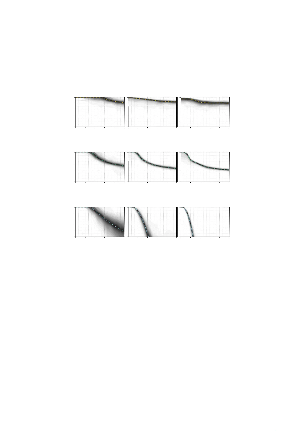
On pa rametric families fo r sampling bina ry data with sp ecified mean and co rrelation Christian Sc h¨ afer 1 , 2 Octob er 25, 2018 W e discuss a class of binary parametric families with conditional probabili- ties taking the form of generalized linear models and sho w that this approac h allo ws to mo del high-dimensional random binary vectors with arbitrary mean and correlation. W e deriv e the sp ecial case of logistic conditionals as an appro ximation to the Ising-type exp onen tial distribution and provide em- pirical evidence that this parametric family indeed outp erforms comp eting approac hes in terms of feasible correlations. Keyw ords Binary parametric families · Sampling correlated binary data 1 Intro duction The need to sample random vectors of correlated binary v ariables arises in v arious sta- tistical application; examples are estimation of the p osterior mean in Bay esian v ariable selection ( George and McCullo c h , 1997 ), small-sample prop erties of estimators in longi- tudinal studies ( F arrell and Rogers-Stew art , 2008 , for a recen t review), stochastic binary optimization in combinatorics ( Rubinstein , 1999 ), sim ulation of ferromagnetic materials ( Sw endsen and W ang , 1987 ), p erformance of neural net works ( Lebbah et al. , 2008 ) and mark et segmen tation analysis ( Dolnicar and Leisc h , 2001 ) among others. Let B := { 0 , 1 } denote the binary space. In some cases, suc h as small-sample analysis in longitudinal studies, w e need a parametric family q explicitly for sampling data on B d with sp ecified mean and correlations. In other cases, the parametric family serves as a proxy for a more complex distribution w e cannot directly sample from. Supp ose we ha ve tw o functions ˜ π : B d → R + and f : B d → R and w e wan t to compute the exp ected v alue E π ( f ( Γ )) = h − 1 P γ ∈ B d f ( γ ) ˜ π ( γ ) with h := P γ ∈ B d ˜ π ( γ ). If d is to o large for enumeration of the state space w e ha ve to rely on Monte Carlo algorithms, the v ast ma jorit y of which in volv e sampling Marko v transitions with inv ari- an t measure π , the standard approac h being the Metrop olis-Hastings k ernel ( Rob ert and Casella , 2004 , c h. 7). F or a transition from X ∼ π := ˜ π /h , we sample Γ ∼ q ( · | X ) from an auxiliary k ernel q and accept the step to Γ with probability λ q ( Γ , X ) := min { 1 , [ ˜ π ( Γ ) q ( X | Γ )] / [ ˜ π ( X ) q ( Γ | X )] } (1) 1 Centre de Recherche en ´ Economie et Statistique, 3 Avenue Pierre Larousse, 92240 Malakoff, France 2 CEntre de REcherches en MAth ´ ematiques de la DEcision, Universit´ e Pa ris-Dauphine, Place du Mar´ echal de Lattre de T assigny 75775 Paris, France or return X otherwise. Random w alks on B d are easy to implemen t but often suffer from slo w mixing; indep endent proposals Γ ∼ q provide fast-mixing if λ q ( Γ , X ) is reasonably high on av erage, in other w ords if q is sufficien tly close to π ( Sch¨ afer and Chopin , 2011 ; Sc h¨ afer , 2012 ). This rationale complements other approaches to fast mixing suc h as parallel chains ( Bottolo and Ric hardson , 2010 , among others) or self-av oiding dynamics ( Hamze et al. , 2011 ). The v ast field of p otential applications in Monte Carlo algorithms encourages the study of families with d ( d + 1) / 2 parameters whic h, lik e the m ultiv ariate normal, accommo date all v alid com binations of means and correlations. This pap er elab orates some theoretical bac kground on random binary v ectors, prov es the range of p ossible correlations for a particular class of parametric families, connects to existing work in the literature and pro vides broad numerical insight concerning the range of dep endencies ac hiev able in practice. It is structured as follows. In Section 2 , we introduce suitable notation and review results relating binary dis- tributions to its momen ts. Section 3 elaborates on parametric families whic h ha v e, b y definition, conditional distributions that are generalized linear regressions. W e show that they accommo date the whole range of p ossible correlations. Section 4 motiv ates the use of the logistic link function as an approximation to the Ising-type exp onen tial quadratic family . In Section 5 , w e discuss how to adjust the parametric families to sp ecified marginals. Finally , in Section 6 w e p erform numerical exp eriments to compare comp eting approaches for sampling correlated binary data in high dimensions. 2 Prelimina ries on random bina ry vecto rs W e write B := { 0 , 1 } for the binary space and denote by d ∈ N the generic dimension. Giv en a v ector γ ∈ B d and an index set I ⊆ D := { 1 , . . . , d } , w e write γ I ∈ B | I | for the sub-v ector indexed by I and γ − I ∈ B d −| I | for its complement. F or I = { i, . . . , j } w e use the more explicit notation γ i : j . Unless otherwise defined, π denotes an arbitrary probabilit y mass function on B d . W e denote b y E π ( f ( Γ )) the expected v alue with resp ect to Γ ∼ π and write P π ( A ) := E π ( 1 A ( Γ )) for an even t A ⊆ B d . Definition Let m ∈ (0 , 1) d b e a mean vector. W e call q u m ( γ ) := Q i ∈ D m γ i i (1 − m i ) 1 − γ i the pro duct family or the mass function of d indep endent Bernoulli v ariables. 2.1 Absolute cross-moments Definition F or a set I ⊆ D , we refer to m π I := E π  Q i ∈ I Γ i  = P γ ∈ B d π ( γ ) Q i ∈ I γ i as the cross-moment indexed by I . Note that m π I = P π ( Γ I = 1 ) which means that cross-momen ts and marginal probabil- ities indexed by I ⊆ D are identical. Higher order cross-moments coincide with first order cross-moments. The range of p ossible cross-momen ts is limited b y the follo wing constrain ts. Prop osition 2.1. The cr oss-moments of binary data fulfil l the sharp ine qualities max  P i ∈ I m i − | I | + 1 , 0  ≤ m I ≤ min { m K : K ⊆ I } . (2) 2 Pr o of. The lo wer b ound follows from | I | − 1 = P γ ∈ B d ( | I | − 1) π ( γ ) ≥ P γ ∈ B d  P i ∈ I γ i − Q i ∈ I γ i  π ( γ ) = P i ∈ I m i − m I , the upp er b ound is the monotonicit y of the measure. F or the sp ecial case | I | = 2, Prop osition 2 is a w ell-kno wn result and has b een inv oked in sev eral articles dealing with correlated binary data. F or the general case, we remark that a mapping f : [0 , 1] | I | → [0 , 1] , f I ( m i 1 , . . . , m i | I | ) = m I , which assigns a cross- momen t m I for I ⊆ D as function of the marginals m i for i ∈ I , is quite similar to a | I | -dimensional copula and the inequalities ( 2 ) are exactly the F r´ echet-Hoeffding b ounds ( Nelsen , 2006 , ch. 2). Definition W e sa y a d × d symmetric matrix M := ( m ij ) with entries in (0 , 1) is a cr oss-moment matrix of binary data if M − diag( M )diag ( M ) | is p ositiv e definite and condition ( 2 ) holds for all I ⊆ D with | I | = 2. W e deriv e the family of distributions whic h, under the constraints that π has giv en cross-momen ts, maximizes the en tropy H ( π ) = − P γ ∈ B d π ( γ ) log [ π ( γ )]. The following prop osition is just a sp ecial case of a more general concept ( So ofi , 1994 ). Prop osition 2.2. L et I ⊆ 2 D b e a family of index sets such that { m I : I ∈ I } is a valid set of cr oss-moments. The maximum entr opy distribution having the sp e cifie d cr oss- moments has the form q ( γ ) = exp( P I ∈I a I Q i ∈ I γ i ) / [ P γ ∈ B d exp( P I ∈I a I Q i ∈ I γ i )] . Pr o of. Define the Lagrange m ultipliers L ( π, a ) = P I ∈I a I [ P γ ∈ B d π ( γ ) Q i ∈ I γ i − m I ] and differen tiate ∂ [ H ( π ) + L ( π , a )] /∂ π ( γ ) = − log[ π ( γ )] − 1 + P I ∈I a I Q i ∈ I γ i . Solving the first order condition and normalizing completes the pro of. 2.2 Standa rdized cross-moments Definition F or a set I ⊆ D , we define u π I ( γ ) := Q i ∈ I ( γ i − m π i )[ m π i (1 − m π i )] − 1 / 2 and refer to c π I := E π ( u π I ( Γ )) as the (generalized) correlation co efficien t indexed by I . A d × d p ositiv e definite matrix C with entries in [ − 1 , 1] and diag ( C ) = 1 is not the correlation matrix of a binary distribution for every mean v ector m ∈ (0 , 1) d . In fact, C is a correlation matrix if and only if M = C · ss | + mm | is v alid in the sense of Definition 2.1 , where the dot means p oin t-wise multiplication and s 2 i := m i (1 − m i ). Chagan ty and Jo e ( 2006 ) elaborate alternative conditions for compatibility betw een correlations and means, but these do not seem easier to express or to chec k. In the con text of binary data, the notion of “strong correlations” refers to correlation co efficien ts which are at the b oundary of the feasible range with resp ect to the mean v ector. Note that the absolute v alue of the correlation co efficient do es, in itself, not tell whether the correlation is easy or difficult to mo del. The follo wing statemen t relates the notions of uncorrelated and indep endent v ariables. Prop osition 2.3. L et X b e a d -dimensional binary r andom ve ctor. F or d = 2 , entries ar e unc orr elate d if and only if they ar e indep endent. F or d ≥ 3 , entries might b e mutual ly unc orr elate d but not indep endent. 3 Pr o of. Let p x 1 x 2 := P ( Γ 1 = x 1 , Γ 2 = x 2 ). By definition p 11 = m 12 = m 1 m 2 . F urther, w e obtain p 10 = m 1 − m 12 = m 1 (1 − m 2 ) and, analogously , p 01 = (1 − m 1 ) m 2 . Finally , w e ha ve p 00 = 1 + m 12 − m 1 − m 2 = (1 − m 1 )(1 − m 2 ). F or d ≥ 3, let for instance p 000 = p 011 = p 101 = p 110 = 1 / 4 and p 100 = p 010 = p 001 = p 111 = 0. The en tries are m utually uncorrelated, but not indep enden t since p 111 = 0 6 = 1 / 8 = m 1 m 2 m 3 . The following represen tation by Bahadur ( 1961 ) allows to write a binary distribution in terms of its generalized correlation co efficien ts. Prop osition 2.4. L et π b e a binary distribution with me an m ∈ (0 , 1) d . Then, π ( γ ) = q u m ( γ ) h P I ⊆ D c π I u π I ( γ ) i . Pr o of. W e give the pro of by Bahadur ( 1961 ) using the notation introduced ab ov e. The set { u π I : I ⊆ D } forms an orthonormal basis on F := { f : B d → R } with resp ect to the inner pro duct ( f , g ) = E q u m ( f ( Γ ) g ( X )) = P γ ∈ B d f ( γ ) g ( γ ) q u m ( γ ) . Therefore, every function f ∈ F has a unique represen tation f ( γ ) = P I ⊆ D ( f , u π I ) u π I ( γ ). Compute the inner pro ducts ( π /q u m , u π I ) = P γ ∈ B d [ π ( γ ) /q u m ( γ )] u π I ( γ ) q u m ( γ ) = E π ( u π I ( Γ )) = c π I to obtain the desired form π ( γ ) /q u m ( γ ) = P I ⊆ D c π I u π I ( γ ). Using Proposition 2.4 , w e ma y bound the l p distance betw een tw o binary distribution with the same mean in terms of nearness of their correlation co efficients. Prop osition 2.5. L et π and ω b e binary distributions with me an m ∈ (0 , 1) d . F or p ≥ 1 , P γ ∈ B d | π ( γ ) − ω ( γ ) | p ≤ P I ⊆ D 2 (1 − min { p, 2 } ) | I | | c π I − c ω I | p ≤ (1 + r ) d − dr − 1 wher e r = 2 1 − min { p, 2 } max I ⊆ D | c π I − c ω I | p/ | I | . Pr o of. Since u π I = u ω I for all I ⊆ D , applying Prop osition 2.4 yields P γ ∈ B d | π ( γ ) − ω ( γ ) | p = P γ ∈ B d    q u m ( γ ) P I ⊆ D u π I ( γ )( c π I − c ω I )    p ≤ P I ⊆ D | c π I − c ω I | p E q u m ( | u π I ( Γ ) | p ) . Using that x p − 1 + (1 − x ) p − 1 ≤ 2 2 − min { p, 2 } for all x ∈ (0 , 1), we obtain the b ound E q u m ( | u π I ( Γ ) | p ) ≤ Q i ∈ I [ m i (1 − m i )] 1 / 2 [ m p − 1 i + (1 − m i ) p − 1 ] ≤ 2 (1 − min { p, 2 } ) | I | . Finally , we ha v e P I ⊆ D 2 (1 − min { p, 2 } ) | I | | c π I − c ω I | p ≤ P I ⊆ D, | I |≥ 2 r | I | = (1 + r ) d − dr − 1, since by definition c π I = c ω I for all I ⊆ D with | I | ≤ 2. Corollary 2.6. L et π and q b e binary distributions with cr oss-moment matrix M . Then we have P γ ∈ B d | π ( γ ) − q ( γ ) | p ≤ (1 + r ) d − 1 2 d ( d − 1) r 2 − dr − 1 . With regard to the Metrop olis-Hastings k ernel men tioned in the in tro ductory section, the factor 1 2 d ( d − 1) r 2 in Corollary 2.6 is the gain of a more complex proposal distribution q M with M = M π = M q o ver a simple pro duct mo del q u m with m = m π = m q . The following result sho ws how the cross-moments of the prop osal distribution affect the auto-cov ariance of the indep endent Metrop olis-Hastings sampler. 4 Prop osition 2.7. L et π and q b e binary distributions with me an m ∈ (0 , 1) d and denote by κ ( γ | x ) := q ( γ ) λ q ( γ , x ) + δ x ( γ )[1 − P y ∈ B d q ( y ) λ q ( y , x )] the Metr op olis-Hastings kernel with invariant me asur e π and pr op osal distribution q wher e λ q ( · , x ) is define d in ( 1 ) . The auto-c ovarianc e b etwe en X ∼ π and Γ ∼ κ ( · | X ) is E κ,π ( Γ X | ) − mm | = 1 2 ( M π − M q ) + R κ with R κ = ( r κ ij ) wher e | r κ ij | ≤ P γ ∈ B d | π ( γ ) − q ( γ ) | . Pr o of. W e plug the definition of the kernel in to the exp ected v alue and obtain E κ,π ( Γ X | ) = X γ , x ∈ B d γ i x j κ ( γ | x ) π ( x ) = X γ , x ∈ B d γ i x j q ( γ ) λ q ( γ , x ) π ( x ) + X x ∈ B d x i x j [1 − P y ∈ B d q ( y ) λ q ( y , x )] π ( x ) = m π ij + X γ , x ∈ B d ( γ i x j − x i x j ) q ( γ ) π ( x ) λ q ( γ , x ) = m i m j + 1 2 ( m π ij − m q ij ) + 1 2 X γ , x ∈ B d ( γ i x j − x i x j ) | q ( γ ) π ( x ) − q ( x ) π ( γ ) | , where w e used 2 q ( γ ) π ( x ) λ q ( γ , x ) = q ( γ ) π ( x ) + q ( x ) π ( γ ) − | q ( γ ) π ( x ) − q ( x ) π ( γ ) | . The triangle inequality X γ , x ∈ B d | q ( γ ) π ( x ) − q ( x ) π ( γ ) | = X γ , x ∈ B d | q ( γ ) π ( x ) − π ( γ ) π ( x ) + π ( γ ) π ( x ) − q ( x ) π ( γ ) | ≤ X γ , x ∈ B d [ | q ( γ ) − π ( γ ) | π ( x ) + | π ( x ) − q ( x ) | π ( γ )] = 2 X γ ∈ B d | π ( γ ) − q ( γ ) | . yields the b ound on r κ ij := 1 2 P γ , x ∈ B d ( γ i x j − x i x j ) | q ( γ ) π ( x ) − q ( x ) π ( γ ) | . 2.3 Structured co rrelations F or some applications, it suffices to mo del structured dep endencies, suc h as exchangeable ( c ij = c ), moving av erage ( c ij = c 1 | i − j | =1 ) or autoregressiv e ( c ij = c | i − j | ) correlations for i 6 = j ∈ D . There is a long series of articles concerned with efficient approac hes to sampling binary v ectors for structured correlations ( F arrell and Sutradhar , 2006 ; Qaqish , 2003 ; Oman and Zuc ker , 2001 ; Lunn and Da vies , 1998 ; Park et al. , 1996 ). In this paper, w e fo cus on the problem of sampling binary data with arbitrary cross-moment matrix. 3 P arametric families based on generalized linea r mo dels W e wan t to construct a parametric family q for sampling independent random vectors with specified mean and correlations. Sampling in high dimensions, ho wev er, requires the computation of conditional distributions q ( γ i | γ 1: i − 1 ), and it is therefore conv enient to define the parametric family directly in terms of its conditionals. 5 Definition Let µ : R → [0 , 1] b e a monotonic function and A := ( a ij ) a d × d real-v alued lo wer triangular matrix. W e refer to q µ A ( γ ) = Q d i =1 h µ ( a ii + P i − 1 j =1 a ij γ j ) i γ i h 1 − µ ( a ii + P i − 1 j =1 a ij γ j ) i 1 − γ i , as the µ -conditionals family . Prop osition 3.1. L et µ : R → [0 , 1] b e a monotonic bije ction and m ∈ (0 , 1) d a me an ve ctor. F or A = diag[ µ − 1 ( m )] we have q µ A = q u m . By construction, it is straightforw ard to sample x ∼ q µ A and ev aluate q µ A ( x ) p oint- wise as summarized in Pro cedure 1 . Alternatively , one could sample from an auxiliary distribution ϕ on R d whic h allo ws to compute ϕ ( x i | x 1: i − 1 ) and define a parametric family q τ ,ϕ ( γ ) = R τ − 1 ( γ ) ϕ ( x ) d x through the mapping τ : R d → B d . W e come back to this idea in Section 5.2 . Pro cedure 1 Sampling from a µ -conditionals family x = (0 , . . . , 0) , p ← 1 for i = 1 . . . , d do c ← q µ A ( x i = 1 | x 1: i − 1 ) = µ ( a ii + P i − 1 j =1 a ij x j ), u ← U ∼ U [0 , 1] if u < c then x i ← 1 p ← ( p · c if x i = 1 p · (1 − c ) if x i = 0 end for return x , p Qaqish ( 2003 ) discusses the µ -conditionals family with a truncated linear link function µ ( x ) = min { max { x, 0 } , 1 } . The linear structure allows to compute the parameters by simple matrix in version; on the do wnside, the linear function is truncated and fails to ac- commo date complicated correlation structures. Therefore, Qaqish ( 2003 ) elab orates on conditions that guarantee the linear cond itionals family to be v alid for sp ecial correlation structures. F arrell and Sutradhar ( 2006 ) prop ose a µ -conditionals family with a logistic link func- tion µ ( x ) = 1 / [1 + exp( − x )]. Ho w ever, they only analyze the special case of autoregres- siv e correlation structure. In Section 4 , we further motiv ate the use of the logistic link function which indeed allo ws to mo del any feasible correlation structure as states the follo wing theorem. Theorem 3.2. L et µ : R → [0 , 1] b e a monotonic, differ entiable bije ction and M a d × d cr oss-moment matrix. Ther e is a unique d × d r e al-value d lower triangular matrix A such that P γ ∈ B d q µ A ( γ ) γ γ | = M . Besides the logistic function inv oked ab o ve, p opular link functions include the com- plemen trary log-log function with µ ( x ) = 1 − exp[ − exp( x )] and the probit function with µ ( x ) = (2 π ) − 1 / 2 R x −∞ exp( − y 2 / 2) dy ( McCullagh and Nelder , 1989 , sec. 4.3). W e deriv e t wo auxiliary results to structure the pro of of Theorem 3.2 . Lemma 3.3. F or a cr oss-moment matrix M with me an ve ctor m = diag( M ) , we have  M m m | 1  > 0 . 6 Pr o of. Note that m | M − 1 m − ( m | M − 1 m ) 2 = ( M − 1 m ) | ( M − mm | ) M − 1 m > 0 b e- cause the co v ariance matrix M − mm | is p ositive definite. Dividing b y m | M − 1 m > 0 w e obtain 1 − m | M − 1 m > 0 which yields det  M m m | 1  = det  M 0 0 | 1   I M − 1 m m | 1  = det( M )det  I M − 1 m 0 | (1 − m | M − 1 m )  = det( M )(1 − m | M − 1 m ) > 0 . Therefore, all principal minors are p ositive. Lemma 3.4. L et µ : R → [0 , 1] b e a monotonic, differ entiable bije ction, and denote by B n r = { x ∈ R n | x | x < r 2 } the op en b al l with r adius r > 0 . L et π b e a binary distribution with cr oss-moment matrix M . We write m = diag ( M ) and m ∗ = ( m | , 1) | for the me an ve ctor. Ther e is ε r > 0 such that the function f : B d +1 r → d +1 × i =1 ( ε r , m ∗ i − ε r ) , f ( a ) = X γ ∈ B d π ( γ ) µ ( a d +1 + P d k =1 a k γ k )  γ 1  is a differ entiable bije ction. Pr o of. W e set ε r := max S i ∈ D ∪{ d +1 } n min a ∈ B d +1 r f i ( a ) , m ∗ i − max a ∈ B d +1 r f i ( a ) o . F or i, j ∈ D ∪ { d + 1 } , the partial deriv ativ es of f are ∂ f i ∂ a j = X γ ∈ B d π ( γ ) µ 0 ( a d +1 + P d k =1 a k γ k ) ×            γ i γ j ( i, j ∈ { 1 , . . . , d } ) γ i ( j = d + 1) γ j ( i = d + 1) 1 ( i = j = d + 1) . W e ha ve η r := min a ∈ B d +1 r min γ ∈ B d µ 0 ( a d +1 + P d i =1 a i γ i ) > 0 since µ is strictly monotonic. Then the Jacobian is p ositive for all a ∈ B d r , det f 0 ( a ) = det   X γ ∈ B d π ( γ ) µ 0 ( a d +1 + P d i =1 a i γ i )  γ γ | γ γ | 1    ≥ η d +1 r det  M m m | 1  > 0 , where we applied Lemma 3.3 in the last inequalit y . The or em 3.2 . W e proceed by induction o ver d . F or d = 1, A (1) is a scalar and w e define the µ -conditionals family q µ A (1) via Corollary 3.1 . Supp ose that w e hav e already constructed a µ -conditionals family q µ A ( d ) with d × d low er triangular matrix A ( d ) and cross-momen t matrix M ( d ). W e can add a new dimension to the µ -conditionals mo del 7 q µ A ( d ) without changing M ( d ), since X x ∈ B d +1 q µ A ( d +1) ( x ) xx | = X x ∈ B d +1 q µ A ( d ) ( x 1: d ) xx | h µ ( a d +1 ,d +1 + P d j =1 a d +1 ,j x j ) i x d +1 × h 1 − µ ( a d +1 ,d +1 + P d j =1 a d +1 ,j x j ) i 1 − x d +1 = X γ ∈ B d q µ A ( d ) ( γ ) ( µ ( a d +1 ,d +1 + P d j =1 a d +1 ,j γ j )  γ γ | γ γ | 1  + h 1 − µ ( a d +1 ,d +1 + P d j =1 a d +1 ,j γ j ) i  γ γ | 0 0 | 0  ) = X γ ∈ B d q µ A ( d ) ( γ ) µ ( a d +1 ,d +1 + P d j =1 a d +1 ,j γ j )  0 γ γ | 1  +  M ( d ) 0 0 | 0  F or reasons of symmetry , it suffices to show that there is a ∈ R d +1 suc h that f ( a ) = X γ ∈ B d q A ( d ) ( γ ) µ ( a d +1 + P d i =1 a i γ i )  γ 1  = M ( d + 1) • d +1 , where the r.h.s. denotes the ( d + 1)th column of the augmen ted cross-momen t matrix. There is ε > 0 so that M ( d + 1) • d +1 ∈ × d +1 i =1 ( ε, m ∗ i − ε ) with m ∗ = (diag [ M ( d )] | , 1) whic h implies that a solution is contained in a sufficiently large op en ball B d +1 r ε . W e apply Lemma 3.4 to complete the inductiv e step and the pro of. 4 The logistic conditionals family W e denote by q ` A the logistic conditionals family , that is the µ -conditionals family with logistic link function ` ( x ) := 1 / [1 + exp( − x )]. This parametric family has b een prop osed b y F arrell and Sutradhar ( 2006 ), and in more general terms suggested b y Arnold ( 1996 ). In this section, w e motiv ate why the logistic link function arises somewhat naturally in the context of µ -conditional families. Definition Let A b e a d × d real-v alued low er triangular matrix. W e refer to q e A ( γ ) = exp( h + γ | A γ ) , as the exp onential quadratic family with h := − log [ P x ∈ B d exp( x | A x )]. Prop osition 4.1. If A = diag( a ) , then a ii = ` − 1 ( m ii ) and q e A = q ` A = q u m . The exp onential quadratic family is a natural wa y to design a parametric family and pla ys a central role in physics and life science b eing the w ell-studied Ising mo del on a w eighted complete graph. It links to information theory ( So ofi , 1994 ), log-linear theory for con tingency tables ( Bishop et al. , 1975 , c h. 5) and graphical mo dels ( Cox and W erm uth , 1996 , ch. 2). Finding its mo de is an NP-hard problem and in tensively studied in the field of op eration research ( Boros et al. , 2007 , for a recent review). 8 Prop osition 2.2 states that the exp onential quadratic family is the maximum en trop y distribution on B d ha ving a giv en cross-moment matrix. It app ears to b e the binary analogue of the m ultiv ariate normal distribution which is the maximum en tropy distri- bution on R d ha ving a given cov ariance matrix ( Kapur , 1989 , sec. 5.1.1). W e can read the parameters a ij as Lagrange multipliers or, if i 6 = j , as conditional log o dd-ratios since a ij = log " P q e A ( Γ i = 1 , Γ j = 1 | Γ − i,j ) P q e A ( Γ i = 0 , Γ j = 0 | Γ − i,j ) P q e A ( Γ i = 0 , Γ j = 1 | Γ − i,j ) P q e A ( Γ i = 1 , Γ j = 0 | Γ − i,j ) # . W e might interpret the constant conditional log o dd-ratios as analogue of the constant conditional correlations of the multiv ariate normal distribution ( W ermuth , 1976 ). Despite these similarities to the m ultiv ariate normal distribution, w e cannot easily sample from the exp onen tial quadratic family nor explicitly relate the parameter A to the cross-momen t matrix M . The reason is that the lo wer dimensional marginal distributions are difficult to compute ( Cox , 1972 , (iii)). Prop osition 4.2. The mar ginal distribution of the exp onential quadr atic family is q e A ( γ − d ) = exp  h + γ | − d A − d γ − d + log h 1 + exp( a dd + P d − 1 j =1 a ij γ j i . (3) W e cannot rep eat the marginalization since the m ulti-linear structure is lost. In fact, the following result shows that the logistic conditionals family is precisely constructed suc h that the non-linear term in the ab o v e expression v anishes. Prop osition 4.3. L et A b e a d × d lower triangular matrix. The lo gistic c onditionals family c an b e written as q ` A ( γ ) = exp  γ | A γ − P d i =1 log h 1 + exp( a ii + P i − 1 j =1 a ij γ j ) i . Pr o of. Straightforw ard calculations yield log q ` A ( γ ) = P d i =1 log  [ ` ( a ii + P i − 1 j =1 a ij γ j )] γ i [1 − ` ( a ii + P i − 1 j =1 a ij γ j )] 1 − γ i  = P d i =1  γ i log[ ` ( a ii + P i − 1 j =1 a ij γ j )] + (1 − γ i ) log[1 − ` ( a ii + P i − 1 j =1 a ij γ j )]  = P d i =1  γ i ` − 1 [ ` ( a ii + P i − 1 j =1 a ij γ j )] + log[1 − ` ( a ii + P i − 1 j =1 a ij γ j )]  = P d i =1  γ i ( a ii + P i − 1 j =1 a ij γ j ) − log[1 + exp( a ii + P i − 1 j =1 a ij γ j )]  = P d i =1 P i j =1 a ij γ i γ j − P d i =1 log[1 + exp( a ii + P i − 1 j =1 a ij γ j )] = γ | A γ − P d i =1 log[1 + exp( a ii + P i − 1 j =1 a ij γ j )] , where we used log [1 − ` ( x )] = − log[1 + exp( x )] in the third line. The full conditional probabilit y of the d -dimensional exp onen tial quadratic family is a logistic regression term. Prop osition 4.4. The c onditional distribution of the exp onential quadr atic family is q e A ( γ i = 1 | γ − i ) = ` ( a ii + P i − 1 j =1 a ij γ j + P d j = i +1 a j i γ j ) . 9 Since w e cannot rep eat the marginalization for low er dimensions, w e cannot assess the low er dimensional conditional probabilities whic h are necessary for sampling. W e can, how ever, deriv e a series of appro ximate marginal probabilities that produce a lo- gistic conditionals family whic h is, for low correlations, close to the original exp onen tial quadratic family . This idea go es back to Cox and W erm uth ( 1994 ). Prop osition 4.5. L et c 1 + c 2 x + c 3 x 2 ≈ log[cosh( x )] b e a se c ond or der appr oximation. We may appr oximate the mar ginal distribution q e A ( γ − d ) by an exp onential quadr atic family exp( h ∗ + γ | − d A ∗ γ − d ) with p ar ameters h ∗ := h + log(2) + c 1 + 1 2 a dd , A ∗ := A − d + ( c 2 + 1 2 )diag( a ∗ ) + c 3 a ∗ a | ∗ , wher e a ∗ := ( a d 1 , . . . , a d d − 1 ) | denotes the d th c olumn of A without a dd . Pr o of. W e write the marginal distribution of the exp onen tial quadratic family as q e A ( γ − d ) = exp h h + γ | − d A − d γ − d + 1 2 ( a dd + a | ∗ γ − d ) + log  2 cosh  1 2 ( a dd + a | ∗ γ − d )  i . using the identit y log[1 + exp( x )] = log  exp( 1 2 x )  exp( − 1 2 x ) + exp( 1 2 x )  = 1 2 x + log  2 cosh( 1 2 x )  and approximate the non-quadratic term b y the second order p olynomial log[cosh( 1 2 a dd + 1 2 a | ∗ γ − d )] ≈ c 1 + c 2 a | ∗ γ − d + c 3 ( a | ∗ γ − d ) 2 . W e rewrite the inner pro ducts a | ∗ γ − d + ( a ∗ γ − d ) 2 = γ | − d [diag( a ∗ ) + a ∗ a | ∗ ] γ − d and rear- range the quadratic terms. W e can iterate the pro cedure to construct a logistic conditionals family which is close to the original exp onential quadratic family . How ev er, the function log[cosh( x )] behav es lik e a quadratic function around zero and lik e the absolute v alue function for large | x | . Th us, a quadratic polynomial can only appro ximate log [cosh( x )] well for small v alues of x which means that exp onential quadratic families with strong dep endencies is hard to approximate. Co x and W erm uth ( 1994 ) prop ose a T a ylor approximation whic h fits well around 1 2 a dd and works for w eak correlations. The parameters are c =  log[cosh( 1 2 a dd )]) , 1 2 tanh( 1 2 a dd ) , 1 8 sec h 2 ( 1 2 a dd )  . 5 Sampling bina ry data with sp ecified cross-moment matrix If 2 d − 1 full probabilities are known, w e easily sample from the corresp onding multinomial distribution ( W alker , 1977 ). F or a v alid set of cross-moments m I , I ∈ I , Gange ( 1995 ) prop oses to compute the full probabilities using a v ariant of the Iterative Prop ortional Fitting algorithm ( Hab erman , 1972 ). While there are no restrictions on the range of dep endencies, we hav e to enumerate the entire state space which limits this v ersatile approac h to low dimensions. In the sequel, we do not consider metho ds for structured correlations nor approac hes whic h require en umeration of the state space. First, we show how to compute the parameter A of a µ -conditionals mo del for a given cross-momen t matrix M . Secondly , w e review an alternative approach to sampling binary data based on the m ultiv ariate normal distribution ( Emrich and Piedmonte , 1991 ). 10 5.1 Fitting the conditionals family The pro of of Theorem 3.2 suggests an iterative pro cedure to adjust the parameter A to a giv en cross-moment matrix M . W e add new cross-moments m ∈ (0 , 1) d +1 to the d × d a low er triangular matrix A by solving the non-linear equation f ( a ) = m via Newton-Raphson iterations a ( k +1) = a ( k ) − [ f 0 ( a ( k ) )] − 1 [ f ( a ( k ) ) − m ] where f ( a ) = P γ ∈ B d q µ A ( γ ) µ [( γ | , 1) a ]( γ | , 1) | f 0 ( a ) = P γ ∈ B d q µ A ( γ ) µ 0 [( γ | , 1) a ]( γ | , 1) | ( γ | , 1) F or dimensions d > 10, the exact computation of the expectations becomes expensive, and we replace f and f 0 b y their Monte Carlo estimates ˆ f ( a ) = P n k =1 q µ A ( γ ) µ [( x | k , 1) a )]( x | k , 1) ˆ f 0 ( a ) = P n k =1 q µ A ( γ ) µ 0 [( x | k , 1) a )]( x | k , 1) | ( x | k , 1) (4) where x 1 , . . . , x n are drawn from q µ A . Some remarks are in order. • If the smallest eigen v alue of M − diag( M )diag ( M ) | approac hes zero or a cross- momen t m ij approac hes the b ounds ( 2 ), the parameter a ij ma y become very large in absolute v alue. The limited n umerical accuracy a v ailable on a computer inhibits sampling from such extreme cases. • W e might encounter n umerical trouble in the course of the fitting pro cedure. In order to circumv ent problems, we set m ij ( λ k ) := λ k m ij + (1 − λ k ) m ii m j j , 0 = λ 1 < · · · < λ n = 1 for all j = 1 , . . . , i − 1 and compute a sequence of solutions a ( λ k ) to the cross- momen ts m ( λ k ). W e stop if the parameters fail to con verge whic h ensures that the mean of the µ -conditionals family is alwa ys diag ( M ). • If we hav e data a v ailable instead of cross-moments, we would rather fit the fam- ily via comp onent-wise lik eliho o d maximization which is usually faster than the metho d of moments and can ev en b e parallelized ( Sch¨ afer and Chopin , 2011 ). • F or the linear link function µ ( x ) = x , we obtain f ( a ) = h P γ ∈ B d q µ A ( γ )( γ | , 1) | ( γ | , 1) i a =  M m m | 1  a whic h alw a ys has a solution b y virtue of Lemma 3.3 ; to construct a mass function, ho wev er, we hav e to fall back to the truncated v ersion µ ( x ) = min { max { x, 0 } , 1 } , and the range of feasible cross-moments is hard to assess ( Qaqish , 2003 ). 5.2 Fitting the Gaussian copula family Emric h and Piedmon te ( 1991 ) prop ose to dichotomize a multiv ariate Gaussian distribu- tion for sampling m ultiv ariate binary data. 11 Definition F or a vector a ∈ R d and a d × d correlation matrix Σ we define the Gaussian copula family q g c a , Σ ( γ ) = R τ − 1 a ( γ ) ϕ Σ ( x ) d x , ϕ Σ ( x ) = (2 π ) − d/ 2 | Σ | − 1 / 2 exp  − 1 2 x | Σ − 1 x  , where τ a ( x ) :=  1 ( −∞ ,a 1 ] ( x 1 ) , . . . , 1 ( −∞ ,a d ] ( x d )  . F or all I ⊆ D , the marginals are m I = P γ ∈ B d q g c a , Σ ( γ ) Q i ∈ I γ i = P γ ∈ B d , γ I = 1 R τ − 1 a ( γ ) ϕ Σ ( v ) d v = R S γ ∈ B d , γ I = 1 { τ − 1 a ( γ ) } ϕ Σ ( v ) d v = R × d i =1    ( −∞ ,a i ] i ∈ I ( −∞ , ∞ ) i / ∈ I ϕ Σ ( v ) d v = Φ ( I ) Σ ( a I ) , where Φ ( I ) Σ is the marginal cum ulative distribution function of the m ultiv ariate Gaussian. W e set a i = Φ − 1 ( m i ) for i ∈ D to adjust the mean. In order to compute the parameter Σ that yields the desired cross-momen ts M , we may use a fast series approximations ( Drezner and W esolo wsky , 1990 ) to solv e m ij = Φ σ ij ( a i , a j ) for σ ij via Newton-Raphson iterations σ r +1 ij = σ r ij − [Φ σ r ij ( a i , a j ) − m ij ] /ϕ σ r ij ( a i , a j ); Mo darres ( 2011 ) suggests the biv ariate Plac kett ( 1965 ) distribution as a pro xy for ϕ σ ij whic h migh t provide a go o d starting v alue σ 0 ij ∈ ( − 1 , 1). While w e alwa ys obtain a solution in the biv ariate case, it is w ell-known that the resulting matrix Σ is not necessarily p ositive definite due to the range of the Gaussian copula which allows to attain the b ounds ( 2 ) for d ≤ 2, but not for higher dimensions. In that case, w e can replace Σ by Σ ∗ = ( Σ + | λ | I ) / (1 + | λ | ) > 0 (5) where λ is smaller than any eigen v alue of Σ . Alternatively , we can pro ject Σ into the set of correlation matrices; see Higham ( 2002 ) and follow-up papers for algorithms that compute the nearest correlation matrix in F rob enius norm. The point-wise ev aluation of q g c a , Σ ( γ ) requires the computation of m ultiv ariate normal probabilities, that is high-dimensional integrals with the resp ect to the density of the m ultiv ariate normal distribution. This is a computationally c hallenging task in itself (see e.g. Genz and Bretz , 2009 ), and the Gaussian copula family is therefore not easily incorp orated in to the Mark ov c hain Monte Carlo algorithms briefly discussed in the in tro duction. 6 Numerical exp eriments In this section, w e compare the µ -conditionals family with truncated linear and logistic link function to the Gaussian c opula family . W e dra w random cross-momen t matrices of v arying dimension and difficult y , fit the parametric families and record how well the desired correlation structure can b e repro duced on av erage. 6.1 Random cross-moments W e first sample the mean m = diag ( M ) ∼ U (0 , 1) d . F or the off-diagonal elemen ts, we ha ve to ensure that the co v ariance matrix M − mm | is p ositive definite and that the constrain ts ( 2 ) are all met. W e alternate the following t wo steps. 12 • P erm utations m ij = m σ ( i ) σ ( j ) for i, j ∈ D with uniform σ ∼ U S ( D ) where w e denote b y S ( D ) := { σ : D → D , σ is bijectiv e } the set of all p ermutations on D . • Replacemen ts m id = m di ∼ U [ a i ,b i ] for all i = σ (1) , . . . , σ ( d − 1) with uniform σ ∼ U S ( D \{ d } ) where the b ounds a i , b i are sub ject to the constraints det( M ) > 0 and min { m ii + m dd − 1 , 0 } ≤ m id ≤ max { m ii , m dd } . The replacemen t step needs some consideration. W e denote by N the in verse of the ( d − 1) × ( d − 1) upper sub-matrix of M and define τ i := m di P i ∈ D \{ d } m d j n ij suc h that det( M ) = [1 / det( N )]( m dd − P i ∈ D \{ d } τ i ) . If we replace m di = m id b y x i w e hav e to ensure that det[ M ( x i )] = det( M ) + m di ( m di n ii + 2 τ i ) − x i ( x i n ii + 2 τ i ) > 0 whic h means ( x i + τ i /n ii ) ∈ ( − c i , c i ) with c i := [ τ 2 i /n 2 ii + det( M ) + m di ( m di n ii + 2 τ i )] − 1 / 2 . Therefore, the low er and upp er b ounds, a i := max { m ii + m dd − 1 , 0 , − τ i /n ii − c i } and b i := min { m ii , m dd , − τ i /n ii + c i } , resp ect all constraints on x i . W e rapidly up date the v alue of the determinan t det[ M ( x i )] and pro ceed with the next entry . W e p erform 10 · d p erm utation steps and run 500 sweeps of replacemen ts b etw een p erm utations. The result is appro ximately a uniform draw from the set of feasible cross- momen ts matrices. Ho w ever, sampling according to thes e cross-moments might not b e p ossible in higher dimensions b ecause the cross-moment matrix is likely to con tain extreme cases whic h are b ey ond the scop e of the parametric family or not w ork able for n umerical reasons. W e in tro duce a parameter % ∈ [0 , 1] which gov erns the difficulty of the sampling problem b y shrinking the upp er and low er b ounds a and b of the uniform distributions to a % := [(1 + % ) a + (1 − % ) b ] / 2 and b % := [(1 − % ) a + (1 + % ) b ] / 2, resp ectively . 6.2 Figure of merit Let M b e a cross-moments matrix and let M ∗ denote the cross-moment matrix with mean m = diag ( M ) and uncorrelated en tries m ∗ ij = m ii m j j for all i 6 = j ∈ D . F or a parametric family q θ , we define the figure of merit τ q ( M ) := ( k M − M ∗ k − k M − M q k ) / k M − M ∗ k , (6) where M q denotes the sampling cross-momen t matrix of the parametric family with parameter θ adjusted to the desired cross-moment matrix M . The norm k · k might b e an y non-trivial matrix norm; in our n umerical exp erimen ts we use the sp ectral norm k A k 2 2 := λ max ( A | A ), where λ max deliv ers the largest eigenv alue, but w e found the F rob enius norm k A k 2 F := tr ( AA | ) to provide qualitativ ely the very same picture. 6.3 Computational results F or fitting the logistic conditionals family when d > 10, w e replace the exact terms by Mon te Carlo estimates ( 4 ) where we use n = 10 4 random samples. W e estimate the cross-momen t matrix of the parametric family q by M q ≈ n − 1 P n k =1 x k x | k where w e use n = 10 6 samples from q . This concerns only the logistic and linear conditionals families; for the Gaussian copula family , we can explicitly compute the sampling cross-moments as m q ij = Φ 2 ( µ i , µ j ; σ ij ), where Σ is the adjusted correlation matrix of the underlying m ultiv ariate normal distribution made feasible via ( 5 ). W e loop ov er 15 lev els of difficult y % ∈ [0 , 1] in 3 dimensions d = 10 , 25 , 50, and gener- ate at eac h time 200 cross-moments matrices. W e denote b y τ 1 ≤ · · · ≤ τ 200 the ordered figures of merit of the random cross-momen t matrices. W e rep ort the median and the 13 quan tiles ( τ b (0 . 5 − ω ) n c , τ d (0 . 5+ ω ) n e ), depicted as underlying gray areas for 20 equidistant v alues of ω ∈ [0 . 0 , 0 . 5]. Figures 1-3 show the results group ed by parametric families; the y -axis with the scale on the left represen ts the figure of merit τ ∈ [0 , 1], the x -axis represen ts the lev el of difficult y % ∈ [0 , 1], and the [0 . 0 , 0 . 5]-gray-scale on the right refers to the level of the quan tiles. Figure 1: Logistic conditionals family d = 10 d = 25 d = 50 0.0 0.2 0.4 0.6 0.8 1.0 0.0 0.2 0.4 0.6 0.8 1.0 ● ● ● ● ● ● ● ● ● ● ● ● ● ● ● ● 0.0 0.1 0.2 0.3 0.4 0.5 0.0 0.2 0.4 0.6 0.8 1.0 0.0 0.2 0.4 0.6 0.8 1.0 ● ● ● ● ● ● ● ● ● ● ● ● ● ● ● ● 0.0 0.1 0.2 0.3 0.4 0.5 0.0 0.2 0.4 0.6 0.8 1.0 0.0 0.2 0.4 0.6 0.8 1.0 ● ● ● ● ● ● ● ● ● ● ● ● ● ● ● ● 0.0 0.1 0.2 0.3 0.4 0.5 Figure 2: Gaussian copula family d = 10 d = 25 d = 50 0.0 0.2 0.4 0.6 0.8 1.0 0.0 0.2 0.4 0.6 0.8 1.0 ● ● ● ● ● ● ● ● ● ● ● ● ● ● ● ● 0.0 0.1 0.2 0.3 0.4 0.5 0.0 0.2 0.4 0.6 0.8 1.0 0.0 0.2 0.4 0.6 0.8 1.0 ● ● ● ● ● ● ● ● ● ● ● ● ● ● ● ● 0.0 0.1 0.2 0.3 0.4 0.5 0.0 0.2 0.4 0.6 0.8 1.0 0.0 0.2 0.4 0.6 0.8 1.0 ● ● ● ● ● ● ● ● ● ● ● ● ● ● ● ● 0.0 0.1 0.2 0.3 0.4 0.5 Figure 3: T runcated linear conditionals family d = 10 d = 25 d = 50 0.0 0.2 0.4 0.6 0.8 1.0 0.0 0.2 0.4 0.6 0.8 1.0 ● ● ● ● ● ● ● ● ● ● ● ● ● ● ● ● 0.0 0.1 0.2 0.3 0.4 0.5 0.0 0.2 0.4 0.6 0.8 1.0 0.0 0.2 0.4 0.6 0.8 1.0 ● ● ● ● ● ● ● ● 0.0 0.1 0.2 0.3 0.4 0.5 0.0 0.2 0.4 0.6 0.8 1.0 0.0 0.2 0.4 0.6 0.8 1.0 ● ● ● ● ● 0.0 0.1 0.2 0.3 0.4 0.5 6.4 Discussion While Theorem 3.2 suggests that the scop e of the logistic conditionals family is far b e- y ond comp eting approaches, we cannot, in practice, exp ect a binary parametric family with d ( d − 1) / 2 dep endency parameters to pro duce just any desired correlation structure. Ho wev er, the practical scop e of the logistic family is limited only b y the a v ailable n umer- ical accuracy while the scope of comp eting metho ds is also limited b y their mathematical structure. The truncated linear conditionals family is fast to compute but its qualit y deteriorates rapidly with growing complexit y . The Gaussian copula family is guaran teed to ha ve the correct mean but it is less flexible than the logistic conditionals family; b esides, it do es not allo w for p oin t-wise ev aluation of its mass function. The logistic conditionals family is computationally demanding but by far the most v ersatile option. These findings confirm similar comparisons carried out against the backdrop of particular applications ( F arrell and Rogers-Stewart , 2008 ; Sch¨ afer , 2012 ). 14 7 Ackno wledgements This w ork is part of the author’s Ph.D. thesis at CREST under sup ervision of Nicolas Chopin whom I would lik e to thank for numerous discussions on this topic. I thank Ioannis Kosmidis for his comments on a prior v ersion of this pap er. References Arnold, B. (1996). Distributions with logistic marginals and/or conditionals. L e ctur e Notes-Mono gr aph Series , 28:15–32. Bahadur, R. (1961). A represen tation of the joint distribution of resp onses to n dichoto- mous items. In Solomon, H., editor, Studies in Item Analysis and Pr e diction , pages pp. 158–68. Stanford Univ ersity Press. Bishop, Y., Fienberg, S., and Holland, P . (1975). Discr ete multivariate analysis: The ory and Pr actic e . Cambridge, MA: MIT Press. Boros, E., Hammer, P ., and T av ares, G. (2007). Lo cal searc h heuristics for quadratic unconstrained binary optimization (QUBO). Journal of Heuristics , 13(2):99–132. Bottolo, L. and Richardson, S. (2010). Evolutionary sto chastic searc h for Bay esian mo del exploration. Bayesian Analysis , 5(3):583–618. Chagan ty , N. and Joe, H. (2006). Range of correlation matrices for dependent Bernoulli random v ariables. Biometrika , 93(1):197–206. Co x, D. (1972). The analysis of m ultiv ariate binary data. Applie d Statistics , pages 113–120. Co x, D. and W erm uth, N. (1994). A note on the quadratic exp onen tial binary distribu- tion. Biometrika , 81(2):403–408. Co x, D. and W erm uth, N. (1996). Multivariate dep endencies: Mo dels, analysis and interpr etation , v olume 67. Chapman & Hall/CRC. Dolnicar, S. and Leisc h, F. (2001). Behavioral market segmentation of binary guest sur- v ey data with bagged clustering. Artificial Neur al Networks—ICANN 2001 , 2130:111– 118. Drezner, Z. and W esolowsky , G. O. (1990). On the computation of the biv ariate normal in tegral. Journal of Statistic al Computation and Simulation , 35:101–107. Emric h, L. and Piedmonte, M. (1991). A metho d for generating high-dimensional mul- tiv ariate binary v ariates. The Americ an Statistician , 45:302–304. F arrell, P . and Rogers-Stew art, K. (2008). Metho ds for generating longitudinally corre- lated binary data. International Statistic al R eview , 76(1):28–38. F arrell, P . and Sutradhar, B. (2006). A non-linear conditional probability mo del for generating correlated binary data. Statistics & pr ob ability letters , 76(4):353–361. 15 Gange, S. (1995). Generating Multiv ariate Categorical V ariates Using the Iterative Prop ortional Fitting Algorithm. The Americ an Statistician , 49(2). Genz, A. and Bretz, F. (2009). Computation of multivariate normal and t pr ob abilities , v olume 195. Springer. George, E. I. and McCullo ch, R. E. (1997). Approaches for Ba yesian v ariable selection. Statistic a Sinic a , 7:339–373. Hab erman, S. (1972). Algorithm AS 51: Log-linear fit for contingency tables. Journal of the R oyal Statistic al So ciety. Series C (Applie d Statistics) , 21(2):218–225. Hamze, F., W ang, Z., and de F reitas, N. (2011). Self-Av oiding Random Dynamics on In teger Complex Systems. T ec hnical rep ort, Higham, N. J. (2002). Computing the nearest correlation matrix — a problem from finance. IMA Journal of Numeric al Analysis , 22:329–343. Kapur, J. (1989). Maximum-entr opy mo dels in scienc e and engine ering . John Wiley & Sons. Lebbah, M., Bennani, Y., and Rogovsc hi, N. (2008). A probabilistic self-organizing map for binary data top ographic clustering. International Journal of Computational Intel ligenc e and Applic ations , 7(4):363–383. Lunn, A. and Davies, S. (1998). A note on generating correlated binary v ariables. Biometrika , 85(2):487–490. McCullagh, P . and Nelder, J. A. (1989). Gener alize d Line ar Mo dels . Chapman & Hall / CRC, London. Mo darres, R. (2011). High dimensional generation of bernoulli random vectors. Statistics & Pr ob ability L etters . Nelsen, R. (2006). An intr o duction to c opulas . Springer V erlag. Oman, S. and Zuc ker, D. (2001). Modelling and generating correlated binary v ariables. Biometrika , 88(1):287. P ark, C., P ark, T., and Shin, D. (1996). A simple metho d for generating correlated binary v ariates. The Americ an Statistician , 50(4). Plac kett, R. (1965). A class of biv ariate distributions. Journal of the Americ an Statistic al Asso ciation , pages 516–522. Qaqish, B. (2003). A family of multiv ariate binary distributions for sim ulating corre- lated binary v ariables with sp ecified marginal means and correlations. Biometrika , 90(2):455. Rob ert, C. and Casella, G. (2004). Monte Carlo statistic al metho ds . Springer V erlag. Rubinstein, R. Y. (1999). The Cross-En trop y Metho d for com binatorial and con tinuous optimization. Metho dolo gy and Computing in Applie d Pr ob ability , 1:127–190. 16 Sc h¨ afer, C. (2012). P article algorithms for optimization on binary spaces. pr e-print . Sc h¨ afer, C. and Chopin, N. (2011). Sequential Mon te Carlo on large binary sampling spaces. Statistics and Computing , to app ear. doi: 10.1007/s11222–011–9299–z. So ofi, E. (1994). Capturing the Intangible Concept of Information. Journal of the A meric an Statistic al Asso ciation , 89:1243–54. Sw endsen, R. and W ang, J. (1987). Nonuniv ersal critical dynamics in monte carlo sim- ulations. Physic al R eview L etters , 58(2):86. W alk er, A. (1977). An efficien t metho d for generating discrete random v ariables with general distributions. A CM T r ansactions on Mathematic al Softwar e , 3(3):256. W erm uth, N. (1976). Analogies b et w een multiplicativ e mo dels in con tingency tables and co v ariance selection. Biometrics , pages 95–108. 17