Fast Calculation of Calendar Time-, Age- and Duration Dependent Time at Risk in the Lexis Space

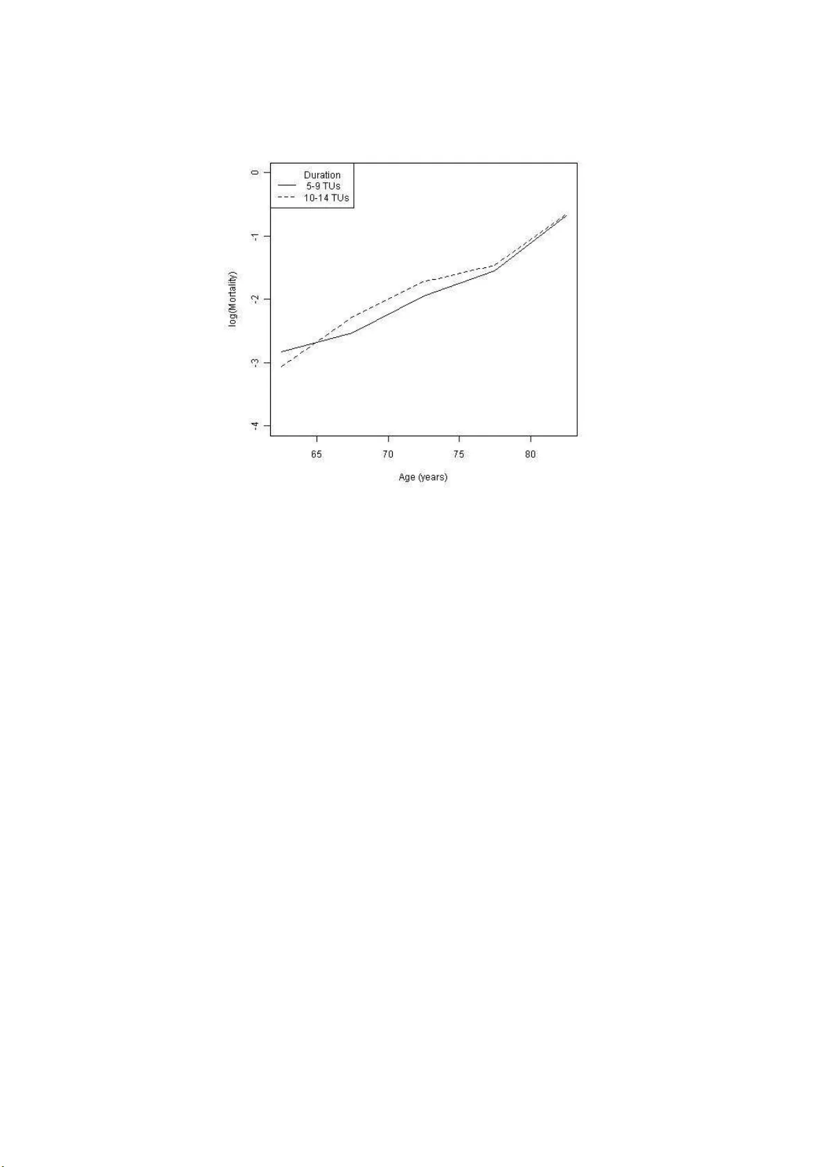
F ast Calculation of Calenda r Time-, Age- and Duration Dep endent Time at Ris k in the Lexis Space Ralph Brinks ∗ Institut e for Biomet ry and Epidem iolog y German Diab et es Center D ¨ usseldorf, Germ an y In epidemiology , the p erson-yea rs metho d is broadly used to estimate the incidence rates of health related ev ents. This needs determination of time at risk stratified b y p erio d , age and sometime s b y duration of disease o r exp osition. The article d escrib es a fast method for calculating the time at risk in t wo - or three-dimensional Lexis diagrams b ased on Siddon’s algorithm. Keywor ds: p erson-y ears method, Lexis diagram, Sidd on’s a lgorithm. 1 Lexis diagram and p erson-y ea rs m etho d In epidemiology , oftentimes relev an t eve n ts or outcomes simulta neously dep end on dif- feren t time scales: age of the su b jects, calendar time and du ration of an ir r ev ers ib le disease. In ev ent history analysis, [5], a useful concept is th e L exis diagr am , whic h is a co-ordinate system with axes calendar time t (abscissa) and age a (ordinate). The calendar t ime dimension sometimes is referred to as p erio d. Eac h sub ject is represented b y a line segmen t from time and age at entry to time and age at exit. Ent ry and exit ma y b e b irth and death, resp ectiv ely , or en try and exit in a epidemiologica l s tudy or trial. There are excellen t and extensiv e in tro ductions ab out the th eory of Lexis d iagrams (see for example [3], [4], [1] and references therein), whic h allo w s to b e sh ort here. When it comes to irreversible diseases, the commonly used t wo-dimensional Lexis diagram with axes in time and age direction may b e generalized to a three-dimensional co-ordinate system with d isease duration d represent ed b y th e app licate (z-a xis). If a su b ject d o es not get the disease during life time, the life line remains in the time-age -plane parallel ∗ rbrinks@ddz.un i-duesseldorf.de 1 to the line b isecting abscissa and ordinate. With other w ord s, the life line for the time without disease p oin ts in the (1 , 1 , 0) direction (where the triple ( t, a, d ) denotes the co-ordinates in time, age and duration d irection, resp ectiv ely). Ho w ev er if at a certain p oin t in time E the disease is diagnosed, the life line c hanges its direction, henceforth p oin ting to (1 , 1 , 1). The situatio n is illustrated in Figure 1 . The life lines of t w o su b jects are sho wn in the three-dimensional Lexis space. At time of b irth (denoted B n , n = 1 , 2) b oth sub jects are d isease-free; b oth life lin es go to the (1 , 1 , 0) dir ection. Th e fi rst su b- ject gets the d isease at E , and henceforth the life line is parallel to (1 , 1 , 1) until death at D 1 . The second sub ject remains without th e disease for th e wh ole life, wh ich ends at D 2 . Figure 1: T h ree-dimensional L exis diagram with t wo life lines. Abscissa, ord inate and applicate repr esen t calendar time t , age a and dur ation d , resp ectiv ely . The life lines start and end at birth B n and d eath D n , n = 1 , 2 . T he fir st sub ject gets the disease at E . Then, th e life line c hanges its dir ection. The s econd sub ject do es n ot get the disease, the corresp ond in g life line r emains in the t - a -plane. In order to measure the frequency of ev en ts in a p opulation, suc h as onset of a c hronic disease, the p erson-y ears metho ds records the num b er of p eople who are affected and the time elapsed b efore the ev en t o ccurs. Th e p erson-y ears incidence rate λ is estimated b y λ = e m , (1) where e is is the num b er of ev ents and m is the n umber of p erson-ye ars at risk [7, p. 250ff]. Calendar time and age often are imp ortan t determinan ts for o ccurr en ce of ev ents and ha v e to b e tak en in to account. This usually is ac hiev ed by dividin g the sub jects’ time sp ent in the stu dy in to calendar time and age groups. Let e ij b e the num b er of ev ents taking place while su b jects are in time and age group ( i, j ) . F urthermore, let m ij 2 b e th e total time at risk sp ent in this group, then Equation (1) b ecomes λ ij = e ij m ij . In the planar Lexis diagram it is clear, h ow the time at r isk m ij can b e obtained. Let the time and age group ( i, j ) b e defined by Cartesian pro du ct S ij := [ t i − 1 , t i ) × [ a j − 1 , a j ). Eac h sub ject whose life line intersects w ith the rectangle S ij con tr ib utes b y its time at risk in S ij . T o b e precise, m ij is the su m of all the sub jects’ times at risk sp en t in S ij : m ij = N X n =1 ℓ ( n ) ij , (2) where ℓ ( n ) ij is the time at risk of sub j ect n, n = 1 , . . . , N , in the rectangle S ij . Again, these ideas can b e generalized to three-dimensional case: Th en, e ij k is the n um b er of even ts taking p lace in the rectangular hexahedron S ij k := [ t i − 1 , t i ) × [ a j − 1 , a j ) × [ d k − 1 , d k ) . F or the times at risk m ij k it h olds m ij k = N X n =1 ℓ ( n ) ij k , (3) where ℓ ( n ) ij k is the time at risk of sub j ect n in volume elemen t S ij k . Giv en a certain study p opulation o f size N , the question a rises ho w the sub jects’ con tr ib utions ℓ ( n ) ij k to the ov erall time at r isk m ij k sp ent in S ij k can b e calculat ed. Since N ma y b e large (up to sev eral thousand), some atten tion sh ould b e paid to computation time. The solution is straigh tforw ard by noti ng that the question is very similar to the problem of f ollo wing a radiological path through a v oxel grid in tomography or ra ytracing in compu ter graph ics. F or b oth fields , tomography and ra ytr acing, there is an ongoing researc h effort to efficie n tly discretize con tinuous lines (radiologi cal paths or rays of ligh t). This article has b een insp ired by the seminal w ork of Sid don, [6]. 2 Intersecting life lines with vo xels in the Lexi s diagram Since the algorithm pr esen ted in this section is motiv ated from the field of computer tomograph y , some of the terminology is u seful. T ypically one of the sets S ij k resulting from a p artition of a r ectangular hexahedron (right cub oid) in to congruent v olume ele- men ts, is called a voxel . The six faces of eac h vo xel are subs ets of t wo adjacen t planes parallel either to t he t - a -plane, a - d -plane or t - d -plane. Hence, th e vo xel space comes along with a set of equid istan t, parallel planes wh ic h are p erp endicular to the abscissa, ordinate or app licate and whic h are defined b y the u nion of all vo xel faces. These planes pla y a cru cial role in the algorithm. 3 In this article all v o xels S ij k are consid er ed to b e cubical, with all edges having the length t r , t r > 0 : S ij k := [ t r · ( i − 1) , t r · i ) × [ t r · ( j − 1) , t r · j ) × [ t r · ( k − 1) , t r · k ) . (4) These vo xels form a grid where the life lines of all sub jects in the study are sorted in to. As a consequence of cubical v oxels, the temp oral r esolution with resp ect to calendar time, age an d dur ation is the same. Ho wev er, generaliza tion to partitions usings rectangular v o xels with height , length and depth b eing different is easily p ossible. The main idea for calculat ing the ℓ ( n ) ij k in the life line L n of sub ject n starting at en try p oint B n := ( t ( n ) 0 , a ( n ) 0 , d ( n ) 0 ), e nding at exit p oin t D n := ( t ( n ) 1 , a ( n ) 1 , d ( n ) 1 ), is the parameterizatio n in th e form L n : B n + α · ( D n − B n ) , α ∈ [0 , 1] . Note, that t ( n ) 1 − t ( n ) 0 = a ( n ) 1 − a ( n ) 0 = d ( n ) 1 − d ( n ) 0 =: ∆ t ( n ) . Using this parameterizatio n, all parameters α ( n ) ∈ [0 , 1] are calculated where an inte rsection with a v o xel face tak es place. Since the v o xels are arranged in a regular grid, in tersecting one of the v o xel faces is equiv alent with intersec ting one of the t - a -, a - d - or t - d -planes formed by the union of all v o xel faces mentioned ab o ve. Hence, we calcula te the inte rsections w ith these planes. Let us start with the a - d -planes (p erp en dicular to the t -axis): all those α ( n ) t where an in tersection with an a - d -plane o ccurs are giv en by α ( n ) t ( u ) = u · t r − ( t ( n ) 0 % t r ) ∆ t ( n ) , u = 1 , . . . , U ( n ) , where % is the m o dulo-op erator and U ( n ) denotes the n um b er of intersected a - d -planes: U ( n ) = j t ( n ) 1 / t r k − j t ( n ) 0 / t r k . Similar formulas hold for those α ( n ) a ( v ) , v = 1 , . . . , V ( n ) , and α ( n ) d ( w ) , w = 1 , . . . , W ( n ) , where L n in tersects the t - d - or t - a -planes, resp ectiv ely . No w define the set A n := { α ( n ) t ( u ) | u = 1 , . . . , U ( n ) } ∪ { α ( n ) a ( v ) | v = 1 , . . . , V ( n ) } (5) ∪ { α ( n ) d ( w ) | w = 1 , . . . , W ( n ) } , whic h con tains those α ( n ) ∈ [0 , 1] where an in tersection o ccurs. No te that th e three sets on the righ t-hand s ide of Eq u ation (5) are not necessarily disjoint . Multiple v alues o ccur if an inte rsection happ ens to b e on an edge or ve rtex of a v o xel. Let A ⋆ n := A n ∪ { 0 , 1 } b e o rdered ascendingly A ⋆ n = { α ( n ) ( p ) | p = 1 , . . . , P ( n ) } with 0 = α ( n ) (1) < · · · < α ( n ) ( P ( n ) ) = 1 . F or calculating the ℓ ( n ) and the asso ciated vo xel indices i, j, k , w e ha ve follo wing algorithm: 1. F or eac h sub ject n , n = 1 , . . . , N , calculate the set A ⋆ n as ab o ve and sort t he elemen ts α ( n ) ( p ) , p = 1 , . . . , P ( n ) , in ascending order. 4 2. F or p = 1 , . . . , P ( n ) set ( i p , j p , k p ) := $ B n + α ( n ) ( p ) · ( D n − B n ) t r % , (6) where th e d ivision is tak en comp onent wise. 3. Then, calculate ℓ ( n ) i p j p k p =  α ( n ) ( p + 1) − α ( n ) ( p )  · ∆ t ( n ) , p = 1 , . . . , P ( n ) − 1 . (7) F or eac h vo xel ( i, j, k ) su mming up all the times ℓ ( n ) ij k , n = 1 , . . . , N , b y Equ ation (3) yields the time at risk m ij k in p erio d-, age- and duration class ( i, j, k ) , wh ic h can b e used in th e p erson-years metho d. The idea of calculati ng the intersecti on p oin ts with th e v o xel faces goes b ac k to Rob ert L. Siddon. The a lgorithm prop osed by Siddon has b een dev elop ed for ra ytracing in tomograph y , wh ere several millions of paths ha v e to b e computed to form a radiological image. While the imp lementati on provi ded with this article is not tuned for efficiency , remark able sp eeding up is p ossible [2]. The execution of 500 runs of an R (The R F ound ation for S tatistica l Compu ting) implement ation of the algorithm with th e data of 200 p atien ts (equiv alen t to a total of 10 5 patien ts) on a 2.6 GHz p ersonal computer tak es 92 seconds. The (simulated) patien t data set is describ ed in more detail in the next section. 3 Exa mples An implem ten tatio n of the metho d in this article h as b een tested with sim ulated patien t data. A study p opu lation of 200 sub jects with entry age 55 to 85 b orn b et w een 0 and 15 (TUs) su ffering from a c hronic d isease for 3 to 15 TUs at is the time of en tr y is assumed to h a ve the mortalit y rate m ( a, d ) = exp( − 10 + 0 . 1 · a ) · (1 + 0 . 1 · d ) . Exit from the s tu dy is assu med to b e only du e to death (no censoring). The aim is to unfold the m ortalit y rate from these patien t data. 5 F or setting u p the data set, follo wing cod e has b een used: for(patN r in 1:200){ thisPatI nAge <- runif(1, 55, 80) thisPatB irth <- runif(1, 0, 15) thisPatD uration <- runif(1, 3, 15) F <- fct_F(thi sPatInAge , thisPatDur ation) thisPatD eathAge <- round( which.mi n(runif(1) > F) + t hisPatInA ge + (runif(1) - 0.5), 3) patMatri x[patNr, ] < - c(thisPatBi rth, th isPatInAge , thisPa tDuration , thisPatD eathAge) } F or the simulatio n of the age of death, inv erse transform sampling is used: ( which.min (runif(1) > F) ). Th erefor the cumulati v e distribution f unction F ( t | a 0 , d 0 ) for someone who ente rs the stud y at age a 0 and ha ving got the disease for d 0 TUs is calculate d in the fun ction fct_F : F ( t | a 0 , d 0 ) = 1 − exp  − Z t 0 m ( a 0 + τ , d 0 + τ )d τ  . If the alorithm is applied to this d ata set with t r = 5 , it is p ossible to estimate the mortalit y rate m ( a, d ) b y the p erson-y ears metho d. T he resu lt is shown in Figure 2. 6 Figure 2: Age- and duration sp ecific mortalit y as estimated by th e p erson-y ears method. 4 Conclusion This article is ab out an extension of the p erson-yea rs wh en p erio d-, age- an d duration- effects o ccur. The metho d to calc ulate the time at risk is based on ra ytracing tec hn iques used in tomograph y and provi des a fast wa y to follo w the individual life lines of sub jects in the L exis diagram. The algorithm is able to treat tw o cases 1. ca lculate the time at risk for n ewly incident cases, and 2. ca lculate the time at risk , where the time elapsed after an ev en t (e.g. duration since onset of a disease) is relev an t. In the first case, the life lines are lo cated in the t - a -plane, in the second the life lines are p oin ting to the (1 , 1 , 1) direction. The later case is imp ortan t, when the duration is a co v ariable. Th is migh t b e the case in late sequalae or mortalit y after h a vin g got a disease. Simila rly , b y interpreting the applicate axis (z-axis) as du ration of exp osur e to a risk factor, th e time at risk dep end ing on p erio d, age and d uration of exp osure can b e calculate d. In large p opulations or register data (log 10 N > 5 , times at risk are usually estimated b y a form u la going b ac k to S v erdrup, [1, Sect. 3.2.]. It is n oted that using the metho d describ ed in this article, estimation is n o longer necessary , b ecause give n ent ry and exit 7 times of the sub jects, c alculation o f times at r isk is p ossible at feasible compu tational exp ense. References [1] Bendix C arstensen. Age-P erio d-Cohort Mo dels for the Lexis Diagram. Statistics in Me dicine , 26(15) :3018– 3045, 2007. [2] Mark Christiaens, Bjorn De S utter, Ko en De Bosschere, Jan V an Camp enhout, and Ignace Lemahieu. A fast, cac he-a w are al gorithm for th e calculation of radiologic al paths exp loiting su b w ord parallelism. In Journal of Systems Ar c hite ctur e, Sp e cial Issue on Par al lel Image Pr o c essing , 1998 . [3] Niels Keiding. Statistical interference in the lexis diagram. Philosophic al T r ansactions of the R oyal So ciety L ondon A , 332:487– 509, 1990 . [4] Niels Keiding. Age-sp ecific incidence and prev alence: a statistical p ersp ectiv e. Jour- nal of the R oyal Statistic al So ciety A , 154:37 1–412 , 199 1. [5] Niels K eiding. Even t h istory analysis an d the cross-section. Statistics in Me dicine , 25(14 ):2343– 2364, 2006. [6] Rob ert L. Siddon. F ast Calculation o f the Exact Radiologic al P ath for a Three- Dimensional C T Arr a y. Me dic al P hysics , 12(2):252– 255, 1985. [7] Mark W o o d w ard. Epidemiolo gy: Study De sign and Data Analysis . T exts in statistical science. Ch apman & Hall/CR C, 2005. 8