Hidden solitons in the Zabusky-Kruskal experiment: Analysis using the periodic, inverse scattering transform

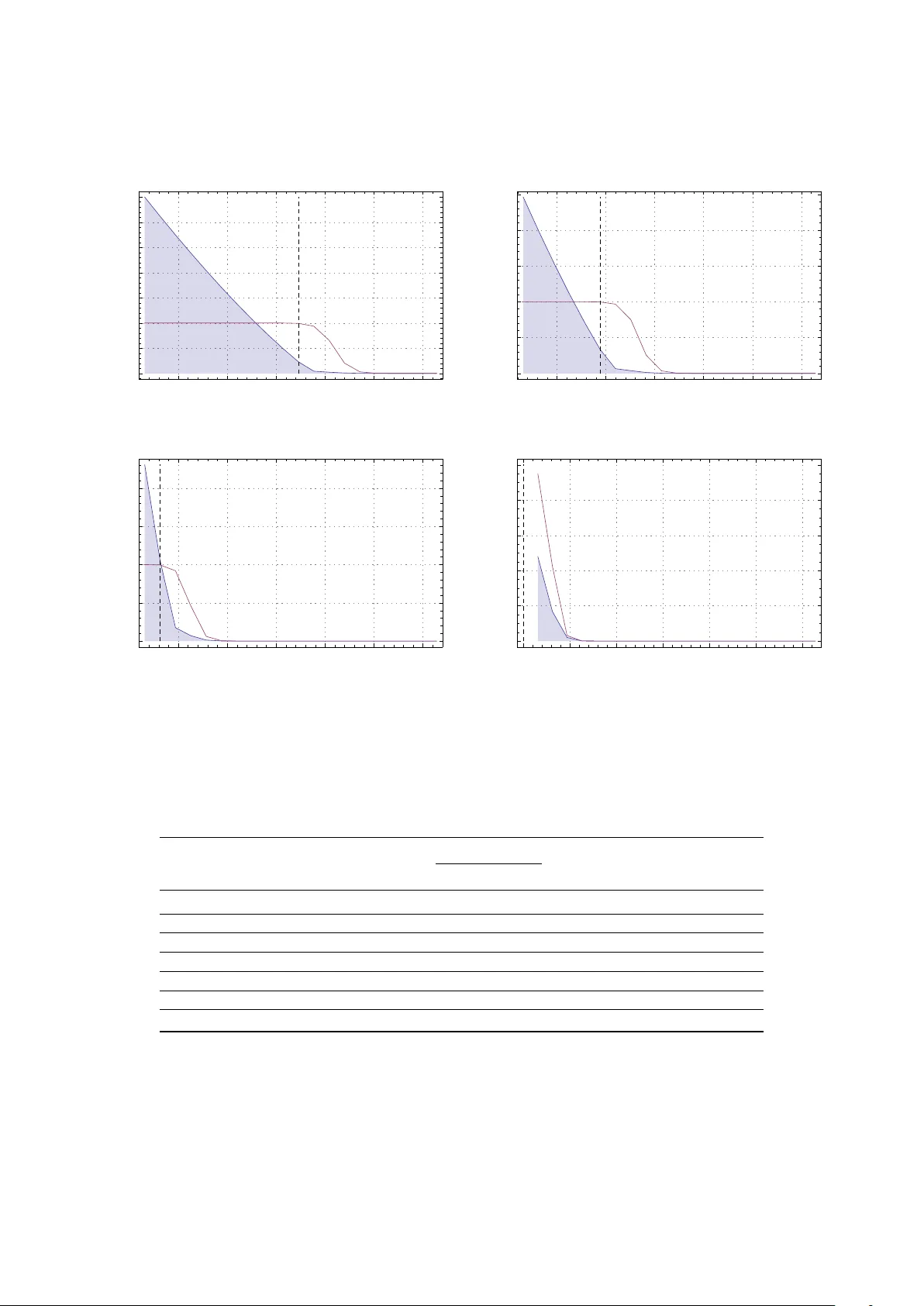
Hidden solitons in the Zab usky–Kruskal e xperiment: Analysis using the periodic, in verse scattering transform Ivan C. Christo v Department of Engineering Sciences and Applied Mathematics, Northwestern University , Evanston, IL 60208-3125, USA Abstract Recent numerical work on the Zab usky–Kruskal e xperiment has re vealed, amongst other things, the existence of hidden solitons in the wa ve profile. Here, using Osborne’ s nonlinear Fourier analysis, which is based on the periodic, in verse scattering transform, the hidden soliton hypothesis is corroborated, and the exact number of solitons, their amplitudes and their reference level is computed. Other “less nonlinear” oscillation modes, which are not solitons, are also found to ha ve nontri vial energy contributions over certain ranges of the dispersion parameter . In addition, the reference le vel is found to be a non-monotone function of the dispersion parameter . Finally , in the case of large dispersion, we show that the one-term nonlinear Fourier series yields a very accurate approximate solution in terms of Jacobian elliptic functions. K ey wor ds: Hidden solitons, K orteweg–de Vries equation, In verse scattering transform, Nonlinear F ourier analysis P A CS: 05.45.Yv, 02.30.Ik 2000 MSC: 35Q51, 35P25 1. Intr oduction Four decades after the discovery of solitons by Zabusk y and Kruskal (ZK) [35] through a computational experi- ment, the study of the ev olution of harmonic initial data under the Korte weg–de Vries (KdV) equation on a periodic interval is f ar from complete [4]. Beyond the discov ery [35] of the ability of the KdV equation’ s (localized) trav eling- wa ve solutions (termed ‘solitons’) to retain their “identity” (shape, speed) after collisions, modern numerical simula- tions by Salupere et al. of this paradigm equation of solitonics rev eal such exotic features as “hidden” (or “virtual”) solitons [9], emergence of soliton ensembles [32] and long-time periodic patterns of the trajectories [29, 33]. These phenomena ha ve been shown to be generic of nonlinear wa ves, as the y occur under other go verning equations as well [13, 27, 28] This raises the simple, yet quite fundamental, question: How many solitons emerge from a harmonic input? A successful approach to answering this question is based upon discr ete spectr al analysis [10, 30, 31]. The essence of this method is to characterize the solitary waves based on the information inherent in the pseudospectral numerical approximation of the underlying partial di ff erential equation (PDE) [26]. In general, solitary wa ve identification is a di ffi cult problem [15, 36], especially when multiple w av e interactions occur and long time scales are considered. Fortunately , in the case of the ZK e xperiment, the KdV equation has an adv antage o ver other nonlinear wav e equations in that it is integr able , i.e., it can be solved e xactly (in theory) using the in verse scattering transform [1] on both the infinite line and on a periodic interval. In this respect, Osborne’ s nonlinear F ourier analysis [16] provides a natural frame work for applying the periodic, in verse scattering transform (PIST) for the KdV equation to real-world problems. In particular , it overcomes the di ffi culty of the PIST being only a theoretical tool by pro viding a practical numerical implementation of it [17, 19, 24]. Osborne and Bergamasco [21] emplo yed this approach to successfully reproduce the numerical results of Zabusky and Email addr ess: christov@alum.mit.edu (Iv an C. Christov) URL: http://alum.mit.edu/www/christov (Iv an C. Christov) Pr eprint submitted to Mathematics and Computers in Simulation October 29, 2018 Kruskal [35]. The y were able to confirm the number of solitons observed emer ging from a harmonic input and the recurrence time of the initial condition. In present w ork, we employ the same approach to corroborate the numerical results of Salupere et al. regarding hidden solitons. Specifically , the aim here is to determine the hidden modes’ amplitudes and classify them in the hierarchy of solutions to the periodic KdV equation (i.e., as either solitons, cnoidal wav es or harmonic wav es). Conceptually , one may consider this approach as a generalization of some of the ideas in [10, 31]. This paper is organized as follows. In Sec. 2, the physical form of the Korte weg–de Vries equation and its transformation to the form considered in [35] is presented. In Sec. 3, the interpretation of the PIST as nonlinear Fourier analysis is discussed. In Sec. 4, the PIST spectrum of the harmonic initial condition for the KdV equation is shown for v arious values of the dispersion parameter, and the hidden soliton hypothesis is discussed. Sec. 5, in the large-dispersion case, illustrates in more detail how a nonlinear Fourier series is constructed using the PIST . Finally , before concluding in Sec. 7, in Sec. 6 we elaborate on the notion of a soliton reference level for the periodic problem and its dependence on the dispersion parameter . 2. P osition of the problem The KdV equation is ar guably the most famous “soliton-bearing” PDEs, gov erning phenomena as seemingly disparate as the motion of lattices, the collecti ve beha vior of plasmas and the shape of hydrodynamic wav es (see, e.g., [1, 7, 22, 35] and the references therein). The classical context [14] in which it arises is the propagation of “long” wa ves over “shallow” water . (For purposes of the present w ork, we do not need to mak e these terms an y sharper .) Letting η ( x , t ) be the surface elev ation, the KdV equation in the moving frame is η t + c 0 η x + αηη x + βη x xx = 0 , ( x , t ) ∈ [0 , L ] × (0 , ∞ ) , (1) where L ( > 0) is the length of the domain, and the subscripts denote partial di ff erentiation with respect to an indepen- dent variable. In addition, the speed of linear wav es c 0 , the nonlinearity coe ffi cient α and the dispersion coe ffi cient β are constant physical parameters. For surf ace w ater w av es, for e xample, they can be expressed in terms of the channel depth h and the acceleration due to gravity g as follo ws [22]: c 0 = p gh , α = 3 c 0 2 h , β = c 0 h 2 6 . (2) As in [35], we are interested in the periodic Cauchy problem (i.e., the initial-v alue problem subject to periodic boundary conditions). Thus, we have that      η ( x , 0) = η 0 ( x ) , x ∈ [0 , L ] , η ( x + L , t ) = η ( x , t ) , ( x , t ) ∈ [0 , L ] × [0 , ∞ ) . (3) A particularly illustrativ e initial condition, which is the one we focus on in the present study , is the harmonic one: η 0 ( x ) = a cos( ω x ) , ω = 2 π L n , n ∈ Z , (4) where a is an arbitrary (real) constant. Now , while Eq. (1) is in the appropriate form to apply Osborne’ s nonlinear F ourier analysis, it is not in the form originally considered by Zabusk y and Kruskal [35] and the subsequent w orks of Salupere et al. T o make the comparison possible, we introduce the following ne w variables: η ( x , t ) = 1 α u ( ξ , τ ) , x = ( ξ + c 0 t ) mod L , t = τ , β = δ 2 , (5) and for definiteness we take L = 2 cm and n = 1. Upon substituting the latter transformations into Eq. (1), we obtain u τ + uu ξ + δ 2 u ξξ ξ = 0 , ( ξ , τ ) ∈ [0 , 2] × (0 , ∞ ) , (6) 2 and the initial–boundary conditions in Eq. (3) become      u ( ξ , 0) = α a cos( πξ ) , ξ ∈ [0 , 2] , u ( ξ + 2 , τ ) = u ( ξ , τ ) , ( ξ , τ ) ∈ [0 , 2] × [0 , ∞ ) . (7) Clearly , we must choose a = 1 /α to normalize the initial condition as in [35]. Also, we must re write the parameters in Eq. (1) in terms of the known quantities δ and g = 981 cm / s 2 . T o this end, we use the identity β = δ 2 and Eq. (2) to deduce h = 6 δ 2 √ g ! 2 / 5 , c 0 =  6 δ 2 g 2  1 / 5 , α = 3 2 6 δ 2 g 3 ! − 1 / 5 . (8) Finally , we note that the dispersion parameter δ used here is identical to the one in [35], and it is related to the dispersion parameter d l of Salupere et al. via d l = − 2 log 10 ( πδ ). 3. Interpr etation of the PIST as a “nonlinear Fourier transform” Next, we turn to the relationship between the PIST and the (ordinary) Fourier transform, and the interpretation of the former as a nonlinear generalization of the latter . T o this end, first we note that the solution strategy by the scattering transform can be split into two distinct steps: the dir ect pr oblem and the in verse pr oblem . The former consists of solving the eigen value problem H ψ = E ψ, H : = − ∂ 2 ∂ x 2 + V ( x ) , x ∈ [0 , L ] , (9) where V ( x ) : = − λη 0 ( x ) is the “potential, ” λ = α/ (6 β ) is a nonlinearity-to-dispersion ratio, and E ∈ R is a spectral eigen value. Equation (9) has been studied extensi vely: in quantum mechanics it is the celebrated (time-independent) Schr ¨ odinger equation [1], and, in the theory of ODEs, it is known as Hill’ s equation [5]. For periodic “potentials, ” i.e., when V ( x + L ) = V ( x ) ∀ x ∈ [0 , L ] as we hav e assumed, it is well-kno wn that the spectrum of the operator H is divided into tw o distinct sets depending upon the boundary conditions imposed on the eigenfunctions ψ [1, 8, 19]. Thus, it is common to classify the spectral eigen values (also kno wn as the “scattering data”) as belonging to either the main spectrum , which we write as the set {E j } 2 N + 1 j = 1 , or the auxiliary spectrum , which we write as the set { µ 0 j } N j = 1 , where N is the number of degrees of freedom (i.e., oscillations modes [16] or band gaps [8]). On the other hand, the in verse problem consists of constructing the nonlinear F ourier series from the spectrum {E j } ∪ { µ 0 j } using either Abelian hyperelliptic functions [18, 23] or the Riemann Θ -function [3, 20]. In former case, which is the so-called µ -representation of the PIST , the exact solution of Eq. (1), subject to the initial and boundary conditions giv en in Eq. (3), takes the form η ( x , t ) = 1 λ          2 N X j = 1 µ j ( x , t ) − 2 N + 1 X j = 1 E j          . (10) It is important to note that all nonlinear wav es and their nonlinear interactions are accounted for in this linear superposition. Unfortunately , the computation of the nonlinear oscillation modes (i.e., the hyperelliptic functions { µ j ( x , t ) } N j = 1 ) is highly nontri vial; ho wever , numerical approaches hav e been developed [23] and successfully used in practice [22, 25]. Sev eral special cases of Eq. (10) o ff er insight into wh y the latter is analogous to the ordinary Fourier series and aid with the interpretation of the results in the following sections. In the small-amplitude limit, i.e., when max x , t | µ j ( x , t ) |  1, we ha ve µ j ( x , t ) ∼ cos( k j x − ω j t + φ j ), where k j is the wa venumber , ω j is the frequency and φ j the phase of the mode. Therefore, if we suppose that all the oscillation modes fall in the small-amplitude limit, then Eq. (10) reduces to the ordinary Fourier series! This relationship is more than just an analogy , a rig- orous deriv ation of the (ordinary) Fourier transform from the scattering transform, in the small-amplitude limit, is giv en in [17]. Ne xt, if there are no interactions, e.g., the spectrum consists of a single wave (i.e., N = 1), we ha ve 3 µ 1 ( x , t ) = cn 2 ( k 1 x − ω 1 t + φ 1 | m 1 ) , which is a Jacobian elliptic function with modulus m 1 . In fact, it is the well-known cnoidal wave solution of the (periodic) KdV equation [1]. For the hyperelliptic representation of the nonlinear Fourier series, gi ven by Eq. (10), the wa venumbers are com- mensurable with those of the ordinary Fourier series, i.e., k j = 2 π j / L (1 ≤ j ≤ N ) [18]. Ho we ver , this is not the only way to classify the nonlinear oscillations. One can use the modulus m j , termed the “soliton index, ” of each of the hyperelliptic functions, which can be computed from the main spectrum as m j = E 2 j + 1 − E 2 j E 2 j + 1 − E 2 j − 1 , 1 ≤ j ≤ N . (11) Then, each nonlinear oscillation mode can be placed into one of two distinct categories based on its soliton inde x: 1. m j & 0 . 99 ⇒ solitons, in particular, cn 2 ( ζ | m = 1) = sech 2 ( ζ ); 2. m j  1 . 0 ⇒ radiation, in particular , cn 2 ( ζ | m = 0) = cos 2 ( ζ ). For m j not in either distinguished limit abov e, the qualitati ve structure of the nonlinear oscillations is not immediately obvious. Boyd [2] argues that for moderate moduli the polycnoidal wa ve solutions of the KdV equation are actually well-approximated by the first few terms in their Fourier series, showing they are, in f act, not much di ff erent from the linear wa ves of the m j  1 . 0 limit. Furthermore, it can be shown [22, 25] that the amplitudes of the h yperelliptic functions are gi ven by A j =              2 λ ( E ref − E 2 j ) , for solitons; 1 2 λ ( E 2 j + 1 − E 2 j ) , otherwise (radiation) . (12) where E ref = E 2 j ∗ + 1 is the soliton r efer ence level with j ∗ being the lar gest j for which m j ≥ 0 . 99. Then, clearly , the number of solitons in the spectrum is N sol ≡ j ∗ . Finally , we note that the theory of Eq. (9) is quite mature and exact solutions can be obtained for a number of specific forms of the potential V ( x ) [1, 5]. Unfortunately , for the ZK experiment (recall Eq. (4)), we have V ( x ) = − λ a cos( ω x ) for which there is no kno wn closed form solution. All is not lost, ho wever , the essence of Osborne’ s nonlinear Fourier analysis is that a numerical solution of Eq. (9) can be obtained and the details of the PIST carried out in this way . T o this end, we use a modified version of Osborne’ s automatic algorithm [19], as described in [6]. The result is an exact (to any desired numerical precision) representation of the nonlinear Fourier spectrum of any initial condition of the KdV equation. 4. How many solitons in a cosine wave? 4.1. The Zab usky–Kruskal e xperiment Recall that, in Sec. 2 upon switching to the new set of v ariables, we distilled all physical parameters of the KdV equation into the dispersion parameter δ . Therefore, it su ffi ces to v ary δ to establish all possible ways a harmonic initial condition can evolv e under the KdV equation. In this subsection, we analyze the classical ZK experiment, i.e., δ = 0 . 022, using the PIST . T o this end, in Fig. 1, the ordinary and nonlinear Fourier spectra of the harmonic initial condition are presented. Since the ordinary Fourier transform, implemented here using the Fast Fourier T ransform (FFT), does not resolve the temporal e volution of a solution of the KdV equation, the FFT of the solution, which was computed by direct numerical integration of the PDE, is presented at t = 3 . 6 /π . This temporal value was chosen for ease of comparison with [35] and because all observ able solitons are visible in the wav e profile at this instant of time. The FFT spectrum suggests that there are over thirty significant normal modes of the problem, with the majority of the enegry concentrated in three distinct wa ve number bands centered at k ≈ 2 . 5 cm − 1 , k ≈ 25 cm − 1 and k ≈ 47 . 5 cm − 1 . Of course, without further study of the FFT spectrum and its ev olution in time, nothing can be said about the number of solitons present in the solution profile. In contrast, the PIST sho ws exactly eight soliton modes plus other nonlinear waves and radiation. As was sho wn in [21], the PIST spectrum captures precisely the eight solitons observed in [35]. Howe ver , what has never been discussed before are the other (four of them, in fact, as T able 1 belo w shows) nontrivial modes in the spectrum. 4 0 20 40 60 80 100 0.00 0.05 0.10 0.15 0.20 0.25 0.30 0.35 2 Π j ! L " cm " 1 # a j " cm # FFT Spectrum at t # 3.6 t B # 3.6 ! Π ! ! ! ! ! ! ! ! ! ! ! ! ! ! ! ! ! ! ! ! " " " " " " " " " " " " " " " " " " " " 10 20 30 40 50 60 0.0 0.5 1.0 1.5 2.0 2.5 3.0 2 Π j ! L " cm " 1 # ! " A j " cm # , " " m j ∆ $ 0.022 Figure 1: (Color online.) Comparison of the ordinary F ourier spectrum (left panel) at a specific time and the nonlinear Fourier spectrum (right panel) of the original ZK experiment ( δ = 0 . 022). The vertical dashed line in the right panel denotes the wave number of the last true soliton mode. By ‘nontrivial’ we mean their amplitudes are not so small as to hav e negligible ener gy contribution. The discrete spectral analysis approach of Salupere et al. [30, 31] found there e xist at least four hidden “solitons” be yond the eight observable ones. Indeed, in Fig. 1, an additional four modes beyond the “true” soliton ones are easily distinguished (i.e., hav e large enough amplitude). Thus, the hidden “soliton” hypothesis is true. What is more, the PIST naturally classifies these hidden modes within the hierarchy of solutions to the periodic KdV equation; it happens the y are not proper solitons (i.e., they ha ve m j < 0 . 99). Finally , Fig. 1 illustrates a very important point: namely , that the FFT is only useful when analyzing a solution . That is to say , the underlying PDE has to be solved up to some instant of time, and then the spectrum computed from this data. Other tools, that can pro vide both time and frequency resolution, such as the short-time (or windowed ) Fourier transform exist [12], howe ver , the PDE must still be solved in advance. On the other hand, the PIST fully characterizes the initial condition and its evolution . This is due to the fact that the PIST is a formal technique for integrating e xactly the KdV and other such integrable nonlinear w av e equations. 4.2. The e ff ect of dispersion on soliton g eneration It has been shown [10, 30, 31] that the number of solitons detected in the solution of the KdV equation v aries with the dispersion parameter . Indeed, it is well-known that, as the zero-dispersion limit ( δ → 0) is approached, the number of solitons generated by an initial condition gro ws quickly [11]. In Fig. 2, we present the PIST spectra of the solution for a number of representativ e v alues of δ besides the ZK value; these were chosen so that a comparison with [10, 30, 31] is possible. The quantitati ve results from theses figures, and all other ones presented in the his paper , are also summarized in T able 1, which includes the rele v ant data from [10, 30, 31] and the heuristic estimate N sol ≈ 0 . 2 /δ due to Zabusk y [34]. For δ = 0 . 0178999 ( ⇔ d l = 2 . 5), we observ e ele ven solitons and nine non-soliton nonlinear wa ves for a total of twenty w av es generated by the harmonic initial condition. Though this value of δ was too small for the computational e ff orts at the time of the studies in [10, 31], the PIST has no issues whatsoev er with δ → 0. The computational time for the nonlinear Fourier analysis grows only linearly with the number of spectral eigen values, and it is independent of δ . For δ = 0 . 0252843 ( ⇔ d l = 2 . 2), we observe six solitons and eight non-soliton nonlinear wav es. For δ = 0 . 0635112 ( ⇔ d l = 1 . 4), the PIST finds two solitons and six other modes. And, for δ = 0 . 142184 ( ⇔ d l = 0 . 7), there are zero solitons out of a total of five waves in the spectrum. The pattern is clear: as the dispersion parameter increases the e ff ects of nonlinearly weaken and fe wer solitons are produced from the initial harmonic wav e. The number of other non-soliton modes in the spectrum also decreases with δ , from nine at δ = 0 . 0178999 to five at δ = 0 . 142184. Now , returning to T able 1 and comparing the number of solitons N sol giv en by the PIST and the number of visible solitons observed by Salupere et al. (i.e., total minus hidden), we see that all but one of the observed “solitons” in the 5 ! ! ! ! ! ! ! ! ! ! ! ! ! ! ! ! ! ! ! ! " " " " " " " " " " " " " " " " " " " " 10 20 30 40 50 60 0.0 0.5 1.0 1.5 2.0 2.5 3.0 3.5 2 Π j ! L " cm " 1 # ! " A j " cm # , " " m j ∆ $ 0.0178999 ! ! ! ! ! ! ! ! ! ! ! ! ! ! ! ! ! ! ! ! " " " " " " " " " " " " " " " " " " " " 10 20 30 40 50 60 0.0 0.5 1.0 1.5 2.0 2.5 2 Π j ! L " cm " 1 # ! " A j " cm # , " " m j ∆ $ 0.0252843 ! ! ! ! ! ! ! ! ! ! ! ! ! ! ! ! ! ! ! ! " " " " " " " " " " " " " " " " " " " " 10 20 30 40 50 60 0.0 0.5 1.0 1.5 2.0 2 Π j ! L " cm " 1 # ! " A j " cm # , " " m j ∆ $ 0.0635112 ! ! ! ! ! ! ! ! ! ! ! ! ! ! ! ! ! ! ! ! " " " " " " " " " " " " " " " " " " " " 0 10 20 30 40 50 60 0.0 0.2 0.4 0.6 0.8 1.0 2 Π j ! L " cm " 1 # ! " A j " cm # , " " m j ∆ $ 0.142184 Figure 2: (Color online.) Nonlinear Fourier spectra of the harmonic initial condition for four representative values of δ . As before, a vertical dashed line delineates the last soliton mode from the remainder of the spectrum. wa ve profile are indeed solitons, and the last is a highly-nonlinear cnoidal wav e. This shows that across a wide range of δ v alues, as was the case for the ZK e xperiment discussed in the pre vious subsection, the hidden “solitons” are a manifestation of the other nonlinearly interacting non-soliton solutions of the periodic KdV equation. Salupere et al. δ d l round(0 . 2 /δ ) T otal Hidden N N sol N A j > 10 − 3 N m j > 10 − 1 0 . 0178999 2 . 5 11 – – 20 11 15 14 0 . 022 2 . 320854 9 12 3 17 8 12 11 0 . 0252843 2 . 2 8 10 3 14 6 10 9 0 . 0635112 1 . 4 3 4 1 8 2 6 4 0 . 142184 0 . 7 1 2 1 5 0 3 2 0 . 317998 − 8 . 5 × 10 − 4 1 – – 3 0 2 1 1 . 0 − 0 . 9943299 0 – – 3 0 2 0 T able 1: Comparison of the discrete spectral and nonlinear Fourier analyses of hidden “solitons” and extended statistics of the nonlinear Fourier spectrum for all values of δ considered here. Finally , we note that one cannot expect to detect (in, e.g., a numerical e xperiment) all nonlinear oscillation modes 6 the PIST finds. That is, the discrete spectral analysis [10, 31] is inherently limited in its ability to resolv e low am- plitude, or very weakly nonlinear w av es in the spectrum. Therefore, to shed some light on precisely which modes can be detected and why , the last two column of T able 1 show the number N A j > 10 − 3 of modes with amplitudes greater than 10 − 3 and the number N m j > 10 − 1 of modes with elliptic moduli greater than 10 − 1 , respectiv ely . Though these cut- o ff s are largely arbitrary , they are qualitati vely reasonable. Indeed, the total number of “solitons” found by Salupere et al. is either of these numbers, for the v alues of δ considered here. Thus, the “small” and “weak” modes in the spectrum (typically , these are radiation modes) are di ffi cult to resolve through discrete spectral analysis. Howe ver , we hav e sho wn, beyond any doubt, that the discrete spectral analysis properly distinguishes the total number of highly nonlinear oscillation modes, both soliton and otherwise, and that there indeed are hidden modes in the ZK experiment. 5. A note on the large dispersion case Though, from a mathematical point of view , the zero-dispersion ( δ → 0) limit is by far the most interesting distin- guished limit of the KdV equation [11], the lar ge-dispersion one ( δ = O (1)) illustrates very well some of the concepts behind the PIST and Osborne’ s nonlinear Fourier analysis. T o this end, Fig. 3 shows the nonlinear Fourier spectrum of the harmonic initial conditions for tw o large values of δ . Clearly , as δ → 1, there is only one lar ge-amplitude mode, with the remaining tw o modes’ amplitudes approaching zero as δ increases (recall T able 1). Moreo ver , the “de gree of nonlinearity” (i.e., the elliptic modulus m j ) of the leading mode decreases as δ increases, while its amplitude remains the same. This is due to the fact that the terms δ 2 u ξξ ξ and uu ξ in Eq. (6) no w balance asymptotically , and there is no nonlinear steepening of the wa ve profile that leads to the generation of solitons [35]. ! ! ! ! ! ! ! ! ! ! ! ! ! ! ! ! ! ! ! ! " " " " " " " " " " " " " " " " " " " " 0 10 20 30 40 50 60 0.0 0.2 0.4 0.6 0.8 1.0 2 Π j ! L " cm " 1 # ! " A j " cm # , " " m j ∆ $ 0.317999 ! ! ! ! ! ! ! ! ! ! ! ! ! ! ! ! ! ! ! ! " " " " " " " " " " " " " " " " " " " " 0 10 20 30 40 50 60 0.0 0.2 0.4 0.6 0.8 1.0 2 Π j ! L " cm " 1 # ! " A j " cm # , " " m j ∆ $ 1. Figure 3: (Color online.) Nonlinear Fourier spectra of the harmonic initial condition for large values of the dispersion parameter . The v ertical dashed line representing the end of the soliton spectrum is now at k = 0 because solitons do not emerge in the solution for these values of δ . Thus, to a good approximation, N = 1 when δ = O (1). In this case, the solution of the periodic KdV equation takes the follo wing form [18]: u ( ξ , τ ) ≈ 4 A 1 cn 2 ( k 1 ξ + ω 1 τ | m 1 ) + λ − 1 ( ˜ E − 2 E 3 ) , (13) where k 1 = √ E 3 − E 1 is the mode’ s wav enumber , ω 1 = 2 ˜ E k 1 is its frequency , and we have set ˜ E : = P 3 j = 1 E j for con venience. Of course, {E j } 3 j = 1 , A 1 = 0 . 499987 and m 1 = 0 . 0653120 are obtained from the PIST . This approximate solution is compared to the numerical solution of the KdV equation, for δ = 1, in Fig. 4. The agreement between the two is quite good. More importantly , Eq. (13) illustrates a fundamental di ff erence between the infinite-line and periodic v ersions of the IST . Not only does the periodic problem ha ve a much richer solution space (a continuum of solutions expressible as Jacobian elliptic functions), b ut it also requires three spectral eigen values to determine one mode. This means that the infinite-line IST approach in [10, 31], while helpful, cannot capture the full picture of the periodic problem. 7 0.0 0.5 1.0 1.5 2.0 ! 1.0 ! 0.5 0.0 0.5 1.0 Ξ # ! x ! c 0 t " mod L ! cm " u ! Ξ , t " # ΑΗ ! Ξ , t " ! cm " t # 3.6 t B # 3.6 # Π Figure 4: (Color online.) Comparison between the numerical (blue) and approximate PIST solution (dashed green), giv en by Eq. (13), of the large-dispersion KdV equation ( δ = 1). 6. A reference le vel f or the periodic problem Recall that in Eq. (12), we defined the quantity E ref as the soliton refer ence le vel . This idea was first formulated in [21], where Osborne and Bergamasco sho wed that a shift in the reference (or zero) lev el of a multi-soliton solution is mathematically equiv alent to a shift in the ener gy lev el of the last soliton’ s band gap edge with respect to E = 0. This giv es the natural definition E ref = E 2 j ∗ + 1 − 0, where (as in Sec. 3) j ∗ is the largest j for which m j ≥ 0 . 99. Hence, if we know E ref , then we can determine the solitons’ reference propagation level and reference wa venumber for the periodic problem as follow: u ref = − α E ref /λ, k ref = 2 π j ∗ / L . (14) T able 2 gives u ref as a function of the dispersion parameter for all v alues of δ discussed in the preceding sections. Naturally , in the lar ge-dispersion case no solitons form, and the harmonic initial condition’ s shape is largely preserved as it propagates. In this limit, the propagation lev el is most naturally understood as the mean level of the solution. Indeed, it is very close to zero—the mean of a trigonometric function ov er its period. This leads to an important observation: in the presence of lar ge radiation modes in the spectrum, the reference le vel is not simply the minimum of the wa ve profile in the solution. That is to say , the true u ref cannot be observed in the numerical solution of the problem, as the oscillatory radiation modes will continually shift the wav e profile minimum; if they could somehow be “filtered” one would see the “pure” solitons propagating on the le vel giv en by u ref in T able 2. δ 1 . 0 0 . 318 0 . 142 0 . 0635 0 . 0253 0 . 022 0 . 0179 u ref 1 . 29 × 10 − 4 7 . 80 × 10 − 4 0 . 337 − 0 . 483 − 0 . 555 − 0 . 720 − 0 . 844 T able 2: The soliton reference le vel u ref , computed from the PIST spectrum using Eq. (14), for various v alues of the dispersion parameter δ . What is more interesting, ho we ver , is that u ref increases with δ , until at a certain v alue it re verses itself and goes back through zero becoming neg ativ e. As δ → 0, it appears that the PIST predicts that u ref → − 1, which is the “absolute minimum” level observed numerically [10, 30, 31]. This shows that the PIST and direct numerical simulation approaches are consistent, as they should, b ut that the PIST o ff ers a deeper insight into ho w u ref varies with δ , which is quite di ffi cult to infer from the numerical simulation. Finally , we note that the infinite-line in verse scattering transform (IST) was used in [10, 31] to corroborate the discrete spectral analysis (numerical) approach. But, because the periodic problem for the KdV equation is not mathematically equiv alent to the infinite-line problem with an initial condition of compact support, the choice of u ref in [10, 31] had to be made befor e the number of solitons could be calculated. This lead to an artificial dependence of N sol on u ref . Though good results were obtained using an appropriate estimate for u ref , it is clear that the PIST approach, which is the natural one for the periodic problem, giv es an unambiguous way to calculate u ref . 8 7. Conclusion The present work sho ws that the ev olution (“spectrum”) of harmonic initial data under the K ortewe g–de Vries (KdV) equation can be fully and automatically characterized by the periodic, in verse scattering transform (PIST). In particular , within the framew ork of Osborne and Bergamasco [21], the hidden soliton hypothesis of Salupere et al. is corroborated, and the exact number of solitons, their amplitudes and their reference le vel is computed. This o ff ers new insight into the phenomenon because such precise results were not possible through the direct numerical integration of the KdV equation and the discrete spectral analysis approach [9, 10, 26, 29, 30, 31, 32, 33]. In particular , the apparent linear v ariation of the soliton amplitudes with the wa venumber , first discussed in [35], is true for all soliton modes detected by the PIST , over a range of δ v alues. Meanwhile, the remainder of the spectrum consists of other “less nonlinear” oscillation modes, e.g., nonlinearly-interacting cnoidal wa ves. Though the amplitudes of these do not follow the linear trend, they are not negligible, and they are, in f act, what is observed numerically as “hidden solitons. ” It is important to note that the present approach (via the PIST and Osborne’ s nonlinear Fourier analysis) to the problem of soliton formation is complementary to the discrete spectral analysis approach of Salupere et al. While the PIST allo ws for a v ery precise decomposition of the initial condition into the “basis” elements of the nonlinear PDE at hand (in the present case, the KdV equation), it requires that the PDE be fully integrable—a rather stringent stipulation. The discrete spectral analysis approach to soliton formation does not require any a priori mathematical structure of the PDE. Finally , two of the findings of the present work require further in vestigation. First, the non-monotone dependence of u ref on δ is quite unexpected. A detailed study is necessary to identify the mechanism for this. Second, the number N sol of solitons predicted by the PIST is always less than the number of “solitons” found in the numerical solution by Salupere et al. across the entire range of values of δ considered here. This means that most hidden “solitons” are not solitons, per se . Clearly , the richness of the solution space of the periodic KdV equation allows for modes that fall “in-between” solitons and radiation. Whether this distinction can be made using the discrete spectral analysis is a very interesting question that would be very relev ant when studying non-inte grable wa ve equations, for which a nonlinear Fourier transform cannot be constructed, and therefore the distinction between soliton and non-soliton modes cannot be made analytically . Acknowledgments The author is indebted to Prof. Andrus Salupere for introducing him to this problem and many stimulating discus- sions on the subject. A Student A ward from Prof. Thiab T aha, or ganizer of the Sixth IMA CS International Conference on Nonlinear Evolution Equations and W ave Phenomena: Computation and Theory , which allowed the author to present this work at the latter conference, is kindly ackno wledged. This w ork was also supported, in part, by a W alter P . Murphy Fellowship from the Robert R. McCormick School of Engineering and Applied Science at Northwestern Univ ersity . References [1] M. J. Ablowitz, H. Segur , Solitons and the Inv erse Scattering T ransform, SIAM, Philadelphia, 1981. [2] J. P . Boyd, Theta functions, Gaussian series, and spatially periodic solutions of the Korte weg–de Vries equation, J. Math. Phys. 23 (1982) 375–387. [3] J. P . Boyd, S. E. Haupt, Polycnoidal wav es: Spatially periodic generalizations of multiple solitons, in: A. R. Osborne (ed.), Nonlinear T opics in Ocean Physics, Elsevier , Amsterdam, 1991, pp. 827–856. [4] R. Camassa, L. Lee, Complete integrable particle methods and the recurrence of initial states for a nonlinear shallo w-water wa ve equation, J. Comput. Phys. 227 (2008) 7206–7221. [5] C. Chicone, Ordinary Di ff erential Equations with Applications, vol. 34 of T exts in Applied Mathematics, Springer–V erlag, Ne w Y ork, 1999. [6] I. Christov , Internal solitary wa ves in the ocean: Analysis using the periodic, in verse scattering transform, Math. Comput. Simulat. 80 (2009) 192–201. [7] T . Dauxois, M. Peyrard, Physics of Solitons, Cambridge Univ ersity Press, Cambridge, 2006. [8] B. Deconinck, Periodic spectral theory , in: A. Scott (ed.), Encyclopedia of Nonlinear Science, Routledge, Ne w Y ork, 2005, pp. 705–708. [9] J. Engelbrecht, A. Salupere, On the problem of periodicity and hidden solitons for the KdV model, Chaos 15 (2005) 015114. [10] J. Engelbrecht, A. Salupere, J. Kalda, G. A. Maugin, Discrete spectral analysis for solitary wav es, in: A. Guran, G. Maugin, J. Engelbrecht, M. W erby (eds.), Acoustic Interaction with Submerged Elastic Structures — Part II: Propagation, Ocean Acoustics and Scattering, vol. 5 of Series on Stability , V ibration and Control of Systems, Series B, chap. 1, W orld Scientific, Singapore, 2001, pp. 1–40. 9 [11] T . Grav a, C. Klein, Numerical solution of the small dispersion limit of K orteweg–de Vries and Whitham equations, Comm. Pure Appl. Math. 60 (2007) 1623–1664. [12] K. Gr ¨ ochenig, Foundations of time-frequency analysis, Birkh ¨ auser , Boston, 2001. [13] L. Ilison, A. Salupere, Propagation of sech 2 -type solitary wa ves in hierarchical KdV-type systems, Math. Comput. Simulat. 79 (2009) 3314– 3327. [14] J. Korte weg, G. de Vries, On the change of form of long wa ves advancing in a rectangular canal, and on a new type of long stationary w aves, Phil. Mag. 39 (1895) 422–443. [15] W . I. Newman, D. K. Campbell, J. M. Hyman, Identifying coherent structures in nonlinear wa ve propagation, Chaos 1 (1991) 77–94. [16] A. R. Osborne, Nonlinear F ourier analysis, in: A. R. Osborne (ed.), Nonlinear T opics in Ocean Physics, Elsevier , Amsterdam, 1991, pp. 669–699. [17] A. R. Osborne, Nonlinear Fourier analysis for the infinite-interv al Korte weg–de Vries equation I: An algorithm for the direct scattering transform, J. Comput. Phys. 94 (1991) 284–313. [18] A. R. Osborne, Numerical construction of nonlinear w av e-train solutions of the periodic Korte weg–de Vries equation, Phys. Re v . E 48 (1993) 296–309. [19] A. R. Osborne, Automatic algorithm for the numerical in verse scattering transform of the K ortewe g–de Vries equation, Math. Comput. Simulat. 37 (1994) 431–450. [20] A. R. Osborne, Solitons in the periodic Korte weg–de Vries equation, the Θ -function representation, and the analysis of nonlinear, stochastic wav e trains, Phys. Rev . E 52 (1995) 1105–1122. [21] A. R. Osborne, L. Bergamasco, The solitons of Zabusky and Kruskal re visited: Perspectiv e in terms of the periodic spectral transform, Physica D 18 (1986) 26–46. [22] A. R. Osborne, M. Petti, Laboratory-generated, shallo w-water surface wa ves: Analysis using the periodic, inv erse scattering transform, Phys. Fluids 6 (1994) 1727–1744. [23] A. R. Osborne, E. Segre, Numerical solutions of the Korte weg–de Vries equation using the periodic scattering transform µ -representation, Physica D 44 (1990) 575–604. [24] A. R. Osborne, E. Segre, The numerical in verse scattering transform for the periodic Korte weg–de Vries equation, Phys. Lett. A 173 (1993) 131–142. [25] A. R. Osborne, E. Segre, G. Bo ff etta, L. Cavaleri, Soliton basis states in shallo w-water ocean surf ace wa ves, Phys. Rev . Lett. 67 (1991) 592–595. [26] A. Salupere, The pseudospectral method and discrete spectral analysis, in: E. Quak, T . Soomere (eds.), Applied W ave Mathematics, Springer - V erlag, Berlin / Heidelberg, 2009, pp. 301–333. [27] A. Salupere, J. Engelbrecht, Hidden and driven solitons in microstructured media, in: W . Gutkowski, T . A. Kow alewski (eds.), ICT AM04 Abstracts and CD-R OM Proceedings, IPPT P AN, W arsaw , Poland, 2004. URL http://fluid.ippt.gov.pl/ictam04/text/sessions/docs/SM11/11813/SM11_11813.pdf [28] A. Salupere, J. Engelbrecht, O. Ilison, L. Ilison, On solitons in microstructured solids and granular materials, Math. Comput. Simulat. 69 (2005) 502–513. [29] A. Salupere, J. Engelbrecht, P . Peterson, On the long-time behaviour of soliton ensembles, Math. Comput. Simulat. 62 (2003) 137–147. [30] A. Salupere, G. A. Maugin, J. Engelbrecht, Korte weg–de Vries soliton detection from a harmonic input, Phys. Lett. A 192 (1994) 5–8. [31] A. Salupere, G. A. Maugin, J. Engelbrecht, J. Kalda, On the KdV soliton formation and discrete spectral analysis, W av e Motion 23 (1996) 49–66. [32] A. Salupere, P . Peterson, J. Engelbrecht, Long-time behaviour of soliton ensembles. Part I–Emergence of ensembles, Chaos Solitons Fractals 14 (2002) 1413–1424. [33] A. Salupere, P . Peterson, J. Engelbrecht, Long-time behaviour of soliton ensembles. Part II–Periodical patterns of trajectories, Chaos Solitons Fractals 15 (2003) 29–40. [34] N. J. Zabusky , Computational synergetics and mathematical inno vation, J. Comput. Phys. 43 (1981) 195–249. [35] N. J. Zab usky , M. D. Kruskal, Interaction of “solitons” in a collisionless plasma and the recurrence of initial states, Phys. Re v . Lett. 15 (1965) 240–243. [36] N. J. Zabusky , D. Silver , V . Fernandez, V isiometrics and modeling in computational fluid dynamics, Math. Comput. Simulat. 40 (1996) 181–191. 10