A New Position Control Strategy for VTOL UAVs using IMU and GPS measurements

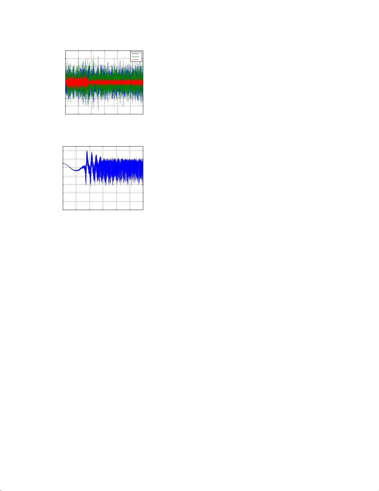
A New P osition Control Strategy for VTOL UA Vs us ing IMU and GPS measure men ts Andrew Rob erts a , Ab delhami d T a y ebi a , b a Dep ar tment of Ele ct ric al and Computer Engine ering, University of Western Ontario, L ondon , Ontario, Canada, N6A 3K7. b Dep ar tment of Ele ctric al Engi ne ering, L akehe ad University, Thunder Bay, Ontario, Canada P7B 5E1 Abstract W e prop ose a new position contro l strategy for VTOL-UA Vs using IMU and GPS measurements. Since there is n o sensor that measures the attitude, our approach does n ot rely on the knowledge (or reconstruction) of the system orientatio n as usually done in the existing literature. Instead, IMU and GPS measuremen ts are directly incorp orated in the control law . An imp ortant feature of the prop osed strategy , is that the accelerometer is used to measure the apparent acceleration of the vehicle, as opp osed to only measuring the gravit y vector, whic h w ould otherwise lead to unexp ected p erformance when the vehicle is accelerating (i.e. not in a h o ver configuration). S im ulation results are provided to demonstrate the p erformance of the prop osed p osition control strategy in th e presence of noise and disturb ances. Key wor ds: VTOL, UA V, vector measurmen ts, p osition contro l, 1 In tro duction The design of po s ition controllers for V ertical tak e- off and landing (VTOL) unmanned airb or ne v ehicles (UA V s) ha s b een the fo cus of several resea rch groups, which has r esulted in significant breakthro ughs in this field, for example see (Abdess a meud and T ay ebi, 201 0), (Aguiar and Hespanha, 2007 ), (F razzoli et al., 200 0), (Hauser et a l., 199 2), (Hua et a l., 200 9), (Pflimlin et al., 2007) and (Ro ber ts and T ay ebi, 2011 a). E xisting p osi- tion cont roller s, usually require tha t the s ystem states are accurately known or measured, na mely the p osition, linear velocity , angular velo city and the o rientation. F o r outdo or applicatio ns a global p ositioning system (GPS) mounted to the sys tem can b e used to pr ovide the p o- sition and velocity meas ur ements, while the angular velocity is obta ined using a gyros cop e which is included in the inertial meas ur ement unit (IMU) in addition to an acc elerometer and a magnetometer. How ever, ther e do es not exist any sensor that pro vides directly the orientation of a r igid bo dy . Motiv ated b y this pro blem, the study of rigid-b o dy attitude estimation has s een sub- ⋆ This pap er was not presented at any IF AC meeting. Cor- respond ing aut hor A . T a yebi. T el. +1 (807) 343-8597. F ax +1 (807) 766-7243. Email addr esses: arober88 @uwo.ca (Andrew R ob erts), atayebi@la keheadu.ca (Ab delhamid T ay ebi). stantial br eakthroug hs due to the efforts of the resear ch communit y (see, for ins tance, (Mahony et al., 2008) ). How ever, we are not aw a re of any work in the liter ature, providing a rigo rous results for the combination of an attitude obser ver and a p os ition controller for VTOL- UA V s. T o a ddress this shortco ming, there ha s b een some effort to design po sition control alg o rithms which do not di- rectly req uire the measure ment of the sy s tem attitude. F or example, in (Rob erts and T ayebi, 2011b) the a uthors prop ose a p ositio n control law which utilizes a num b er of ve ctor me asu r ements as a means to eliminate the requirement for the a ttitude measurement. By v ector measurements w e a re referring to the bo dy-referenced measurements o f vectors whose co ordinates ar e known in the inertial frame. Since the vector measur ement s contain information ab out the system o rientation, it has b een shown that they ca n be applied directly to the p os ition controller thereby eliminating the need o f the observer completely . Consequently , the resulting vector-measurement-based p osition control laws do not require the direct mea surement of the system attitude, nor do they require a n attitude observer which provides practitioners with a simpler, reduced order closed lo op system, with a ccompanying pro ofs for stability . Unfortunately , the vector-meas ur ements based p osi- tion con tr ol str a tegy c a n be susceptible to a problem asso ciated with the la ck of s ensors which can provide Preprint submitted to Automatica 31 Octob er 2018 suitable vector measur ements. This shortcoming stems from the fac t that the t wo sensor s most commonly used to provide vector measurements a re the magneto me- ter and a ccelerometer , used to provide b o dy-r eferenced measurements of the E arths magnetic field and gravity vector, resp ectively . Ho wev er , in order to satisfy the requirement that the accelerometer provides a measure- men t of the gravit y vector only , o ne must a s sume that the b o dy-fixed fra me is no n- accelera ting . It is clear that this condition is not gua ranteed to b e sa tisfied in s ome applications inv olving VTOL UA Vs. Of co urse, this practical limitation is r elev ant to b oth vector-measurement-based p osition controllers and a t- titude obse rvers which use accelerometer s. F ortunately , this limitatio n has led to the development of a new class of a ttitude observers which uses the accelero meter (and magnetometer) to provide v ector-meas urements. This t ype o f observer ac k nowledges the fact that the accelerometer meas ures a combin ation of the gravit y vector and the acceleration of the rigid-bo dy in the bo dy-fixed frame. This combination of the g ravit y vec- tor and linear acceleration in the inertial refere nce frame is commonly referred to as the app ar ent ac c eler ation . This inertial vector vio lates the requirement of many of the v ector-mea surement-based attitude o bs ervers, since the system acceler ation is not known in the iner tial frame of r e ference. In or der to deal with the fact that the inertial vector is unknown, this type of attitude ob- server us e s the velo c it y of the rigid-b o dy (assumed to be measur able using, for instance, a GPS) in addition to the signals o btained from an IMU. The s e attitude observers, which are often re ferred to as velo city-aide d attitude observers , can b e found in (Bonnab el et al., 2008), (Martin a nd Sala ¨ un, 2 008) and (Martin and Sala ¨ un, 2 010) with lo c al stability pro ofs , a nd in (Hua, 2010) with almos t semigloba l sta bilit y res ults. In this pap er we prop ose a new p osition co nt rol ap- proach which obviates the r equirement o f the system attitude measurement by us ing the vector mea s ure- men ts directly in the con tr ol la w. W e spec ifically use a magnetometer and accelerometer to provide the tw o vector measur e ments. The accelerometer is used to mea- sure the system app ar en t ac c eler ation , rather than the gravit y vector only . Using our pr o p osed appro ach, we show that, up on a suitable choice o f the co ntrol gains, all system states remain b ounded, and the system po - sition co nverges to a constant r eference p osition. Our prop osed co nt rol strateg y 1) do es no t requir e direct measurement of the system attitude; 2) do es not requir e the us e of a n attitude o bserver; 3) uses an acceler o meter to pr ovide a vector mea surement without limiting the motion of the s ystem to a near-hover s tate. 2 Bac kground In this section we pr esent some of the necessary mathe- matical details we use througho ut the pap er. In section 2.1 w e descr ib e tw o commonly used attitude representa- tions (r otation matrices and unit-quaternion). In s e ction 2.2 we define functions which are necessa ry in develop- ing the prop os ed control laws. 2.1 Attitude Rep r esentation T o represent the orientation of the air craft (rigid-b o dy), we define tw o refer ence fra mes : An inertial fra me I , which is r igidly attached the Earth (assumed flat), and a b o dy frame B which is rigidly attached to the a ircraft center of gravit y (COG). The orthonor mal basis of B is taken suc h that the x a xis is direc ted tow a rds the front of the air c r aft (or rig id b o dy), the y ax is is taken to- wards the star bo ard (right) side, and the z axis is di- rected down wards (o pp o s ite the dire c tio n of the system thrust). Throughout the pap er we often refer to the orientation of the r igid-b o dy , by which w e mean the relative an- gular p ositio n o f B with resp ect to I . The g oal o f the attitude repres entation is to mathematically desc r ib e the orientation of the rigid-b o dy . The unit-quaternion, which is a unit vector on R 4 , is given by Q = ( η , q ) ∈ Q , where η ∈ R is the quaternion-sca lar and q ∈ R 3 is the quaternion-vector, and Q is the set of unit-q uaternion defined by Q ≡  Q ∈ R × R 3 , k Q k = 1  . (1) Let Q 1 = ( η 1 , q 1 ) ∈ Q , Q 2 = ( η 2 , q 2 ) ∈ Q denote tw o unit-quaternion; then the quaternion pr o duct of Q 1 and Q 2 , denoted b y Q 3 = ( η 3 , q 3 ) ∈ Q is defined b y the following op eratio n Q 3 = Q 1 ⊙ Q 2 =  η 1 η 2 − q T 1 q 2 , η 1 q 2 + η 2 q 1 + S ( q 1 ) q 2  . (2) The set of unit-qua ternion Q forms a gro up with the quaternion m ultiplication op eratio n ⊙ , with the qua ter - nion inv er s e Q − 1 = ( η , − q ), and identit y element (1 , 0 ) = Q − 1 ⊙ Q = Q ⊙ Q − 1 . The unit-qua ternion is an ov e r-para meterization of the the sp ecial group of or- thogonal matrices of dimension three S O (3), defined a s S O (3 ) ≡  R ∈ R 3 × 3 , | R | = 1 , R T R = RR T = I  , (3 ) that is, the tr ansformation from the quaternion s pace Q to S O (3), g iven by the following Ro drigues formula: R ( Q ) = I + 2 S ( q ) 2 − 2 η S ( q ) . (4) where S ( · ) is a skew-symmetric matrix given in the next section, is a tw o-to-o ne map, i.e., R ( Q ) = R ( − Q ). 2.2 Skew symmetric matric es and b ounde d functions Let x, y ∈ R 3 . W e define the skew-symmetric matrix S ( x ) suc h that S ( x ) y = x × y , wher e × deno tes the 2 vector cross pro duct. Several useful properties of this skew-symmetric matr ix are given b elow: S ( x ) 2 = xx T − x T xI 3 × 3 , (5) S ( Rx ) = RS ( x ) R T , R ∈ S O (3 ) , (6) S ( x ) y = − S ( y ) x = x × y , (7) λ  S ( x ) 2  = h 0 , − k x k 2 , −k x k 2 i , (8) where λ ( M ) denotes the eigenv a lue s of the matrix M ∈ R 3 × 3 . Consider the b ounded, differentiable function, denoted as h ( · ) : R 3 → R 3 , which satisfies the following prop er- ties: u T h ( u ) > 0 ∀ u ∈ R 3 , k u k ∈ (0 , ∞ ) , 0 ≤ k h ( u ) k < 1 0 < k φ ( u ) k ≤ 1 ) ∀ u ∈ R 3 , k u k ∈ [0 , ∞ ) , (9) where φ ( u ) := ∂ ∂ u h ( u ). Thro ug hout the pap er we make use of one particular example giv en b y h ( u ) =  1 + u T u  − 1 / 2 u . Using this definition for h ( · ) one c a n derive the ex pr ession φ ( u ) = (1 + u T u ) − 3 / 2 ( I 3 × 3 − S ( u ) 2 ) . . 3 P o sition Co n trol Using GPS and IMU Mea- surements Using the ab ove mathematical background, we will now pro ceed to for mulate the problem and define the pos i- tion control laws. A num b er of steps ar e taken which are group ed into v arious sections. In section 3.1 we define the sys tem mo del. In section 3.2 we formulate the pr ob- lem and state some necess ary a ssumptions. Section 3.3 provides an attitude e x traction a lg orithm which allows us to s pec ify a desir ed sy s tem attitude based up on the v alues o f the p osition and veloc ity error, and sectio n 3.4 defines a ttitude er ror functions. Finally , in section 3.5 we describ e the p osition control laws. 3.1 Equations of Motion T o mo del the system translationa l dynamics, we let p, v ∈ R 3 denote the p ositio n a nd velocity , res p ectively , of the vehicle COG expr essed in the inertial fra me I . F or this problem we assume that the bo dy-r eferenced angular v elo city v ector ω is av ailable a s a control input. W e cons ider the following VTOL UA V mo de l: ˙ p = v , (10) ˙ v = µ + δ, µ = g e 3 − u t R T e 3 , (11) ˙ Q = 1 2 " − q T η I 3 × 3 + S ( q ) # ω , (12) where u t = T /m b , T is the system thrust, m b is the sys- tem mass, e 3 = co l [0 , 0 , 1], g is the gravitational a ccel- eration, a nd δ is a dis tur bance which is dependent on aero dynamic drag forces. The control input of the s ys- tem is defined as u = [ u t , ω ] T . The system output is de- fined as y = [ p, v , b 1 , b 2 ] T where b 2 is the sig na l obtained using an accelero meter, b 1 = Rr 1 is a signal o btained using a ma gnetometer, a nd r 1 is the magnetic field of the surrounding en vironment (assumed consta nt). Note that the system attitude R (or Q ) is not assumed to b e a known output of the sys tem. W e co nsider a well-known mo de l for the a ccelerometer mo del (which includes force s due to linea r acceleratio n ˙ v ) which is given by b 2 = R ( ˙ v − g e 3 ) = − u t e 3 + Rδ = Rr 2 , (13) where r 2 is the inertial r eferenced system appare nt ac- celeration, which s atisfies ˙ v = g e 3 + r 2 , r 2 = − u t R T e 3 + δ. (14) In the development of attitude observers, it is often as- sumed that the system is nea r ho ver (or ˙ v ≈ 0) in or der to ass ume that the acceler ometer measur es the direc- tion of the gr avit y v ector. Also, in most situations the aero dynamic disturba nce vector δ is not included in the mo del. Howev er , for the VTOL UA V mo del, one ca n ea s - ily see that if the a ero dynamic disturbance is neg lected, or we assume tha t δ ≈ 0, then the acceler ometer sig - nal provides the measurement b 2 = − u t e 3 , which is the constant vector e 3 m ultiplied by the system thrust. In this case the use of the a ccelerometer seems trivial since its measurement is known a prior i and do es not co ntain any informatio n ab out the sy s tem attitude. Therefore, we see that for the VTOL UA V system, the as sumption that the a ccelerometer measur e s only the gravit y vector may be a dangerous assumption whic h may lea d to un- exp ected p erforma nce, even in the ca se where ˙ v ≈ 0. In fact, it seems that the utility of the acc e lerometer mea- surements is r elated to the measur ement of the vector δ since the a ccelerometer mea sures b 2 = − u t e 3 + Rδ . F or this rea son we b elieve that it is impor tant to include a mo del of the aero dyna mic disturba nces. 3.2 Pr oblem F ormulation Let p r denote a desired reference p ositio n, which is as- sumed to be constant (or slowly-v arying), and let e p = p − p r . Our main o b jective is to develop a control la w for the system inputs u t and ω , using the av a ilable system outputs y = [ p, v , b 1 , b 2 ], such that the system states e p and v a re b ounded a nd lim t →∞ e p ( t ) = lim t →∞ v ( t ) = 0 . F or the p ositio n control design we first require the fol- lowing assumptions a r e satisfied. 3 Assumption 1 Ther e exist p ositive c onstants c 1 and c 2 such that k r 2 ( t ) k ≤ c 1 and k ˙ r 2 ( t ) k ≤ c 2 . Assumption 2 Given two p ositive c onstants, γ 1 and γ 2 , ther e exists a p ositive c onstant c w ( γ 1 , γ 2 ) such t hat c w < λ min ( W ) wher e W = − γ 1 S ( r 1 ) 2 − γ 2 S ( r 2 ) 2 . The second assumption is satisfied if r 2 is non-v anishing and is no t collinear to the ma gnetic field vector r 1 . In the case where r 2 = 0, the sys tem velocity dynamics b e- come ˙ v = g e 3 (whic h corresp o nds to the r igid bo dy b e- ing in a free-fa ll state) which is not likely in normal cir- cumstances. When this assumption is satisfied, it follows that W is p ositive definite. F urthermo re, if this as sump- tion is satisfied, the v a lue of c w > 0 can b e arbitrar ily increased by increasing the v a lues of γ 1 and γ 2 . In additio n to this assumption, we also r e q uire some con- ditions on the a ero dynamic for ce vector δ . Assumption 3 (Aero dynamic F orces) In light of the fac t that the disturb anc e for c e δ is due to aer o dy- namic for c es exerte d on the vehic le we make the fol lowing simplifyi ng assumptions: (a) The aer o dynamic disturb anc e δ is dissip ative with r esp e ct to the system tr anslational kinetic ener gy and satisfies δ T v ≤ 0 . (b) The aer o dynamic distu rb anc e for c e δ is only dep en- dent on the system tr anslational velo city, and ther e exist a p ositive c onstant c 1 such that k δ k ≤ c 1 k v k 2 (c) Ther e exists p ositive c onstants c 2 and c 3 such that k ˙ δ k < c 2 + c 3 k v k 3 . Assumption 3(a) a nd 3(b) can b e realized when the s ys- tem is op erating in an environment where the ex ogenous airflow is negligible (no wind). Ass umption 3(c) can b e satisfied when the system geometry is sufficiently sym- metrical such that the system aero dynamic forces do not sig nificantly dep end on the sy stem or ientation. Al- though this assumption may b e rea sonable for certain VTOL t ype aircraft, for example the ducted-fan, this as- sumption may not be the case with cer ta in systems, for example fixed wing aircra ft, w he r e the sy stem aer o dy- namics depend largely on the orientation of the vehicle. Now that we hav e es tablished the requir ed assumptions, let us consider the model for the system acceleration from (11). Due to the underactuated nature of this sys - tem, the transla tional a c c eleration is driven by the sys- tem thrust and orientation µ ( u t , R ). Tha t is, if µ was a control input, setting µ = − k p e p − k v v w ould sa tisfy the ob jectives (since v T δ ≤ 0 ). How ever, s ince µ is a func- tion of the system state, we define µ d ∈ R 3 as the desir e d ac c eler ation , and intro duce the new e rror signal ˜ µ = µ − µ d . (15) Subsequently , a new ob jective is to force ˜ µ → 0 in order to obtain the desir ed transla tional dynamics. Since the signal µ is dependent o n the system thrust a nd attitude, based up on the v alue of the desired acceleratio n µ d we wish to o bta in a suitable desir e d attitude , denoted as Q d = ( η d , q d ) ∈ Q , a nd system thrust u t , such that the following equation is satisfied µ d = g e 3 − u t R T d e 3 , (16) where R d = R ( Q d ) is the rotation matrix corresp onding to the unit-quater nion Q d , as defined by (4 ). An extr ac- tion metho d satisfying these requir e ments, whic h has bee n previo usly given in (Rob er ts and T ayebi, 2011a), is describ ed in the fo llowing section. 3.3 Desir e d Attitude and Thrust Extr action In this sec tio n, given a v alue of the desir ed accele r ation µ d , we seek to o btain the v alue o f the desired orientation R d (or equiv alently in terms of the unit-quaternion Q d ) such that equation (16) is satisfied. T o so lve this problem we us e an attitude a nd thrust ex traction algorithm which has been previously prop o s ed by (Rob erts and T ay ebi, 2011a ): Given µ d where µ d / ∈ L , L = { µ d ∈ R 3 ; µ d = col[0 , 0 , µ d 3 ]; µ d 3 ∈ [ g , ∞ ) } , (17) then, one so lution for the thrust u t and attitude Q d = ( η d , q d ) wher e R d = R ( Q d ), which satisfies (16) is g iven by u t = k µ d − g e 3 k , (18) η d =  1 2  1 + g − e T 3 µ d k µ d − g e 3 k  1 / 2 , (19) q d = 1 2 k µ d − g e 3 k η d S ( µ d ) e 3 . (20) The extracted a ttitude Q d has the time-deriv ative ˙ Q d = 1 2 " − q T d η d I 3 × 3 + S ( q d ) # ω d , (21) where the desir e d angular velo city ω d is given b y ω d = M ( µ d ) ˙ µ d , (22) M ( µ d ) = 1 4 η 2 d u 4 t  − 4 S ( µ d ) e 3 e T 3 + 4 η 2 d u t S ( e 3 ) + 2 S ( µ d ) − 2 e T 3 µ d S ( e 3 )  S ( µ d − g e 3 ) 2 . (23) 3.4 Attitude Err or T o repres e n t the relative o rientation of the desired at- titude Q d with res p ect to the actual attitude Q , w e let 4 ˜ Q = ( ˜ η , ˜ q ) ∈ Q and ˜ R = R ( ˜ Q ) ∈ S O (3) denote the un- known attitu de err or which is defined by ˜ Q = Q ⊙ Q − 1 d , ˜ R = R ( ˜ Q ) = R T d R, (24) where Q d is the unit quaternion o bta ined using (19) a nd (20). In lig h t o f ˙ Q and ˙ Q d , a s defined by (12) and (21), resp ectively , the time deriv a tive of the a ttitude error is found to b e ˙ ˜ Q = 1 2 " − ˜ q T ˜ η I + S ( ˜ q ) # ˜ ω , ˙ ˜ R = − S ( ˜ ω ) ˜ R, (25) ˜ ω = R T d ( ω − ω d ) , (26) where ω d is the desi r e d angular velo city as defined by (22). One of the ob jectives of the control desig n is to force the system o rientation to the desired attitude, or in terms of the rotatio n matrices, to for ce R → R d (and therefore µ → µ d ), in order to obtain the desired transla- tional dyna mics. As mentioned in section 2.1, this c orre- sp onds to tw o p oss ible solutions for the unit-quaternion which are given b y ˜ Q = ( ± 1 , 0 ). The m ultiplicit y o f equi- librium solutions is ma nageable since our ob jectives are satisfied for b oth v alues of the unit-quaternio n. 3.5 Position Contr ol ler The p ositio n controller design is based up on a v alue o f the desir e d system transla tio nal acceler ation, which is sp ecified by the virtual control law µ d . Using the ca lcu- lated v alues for the po sition err o r e p = p − p r , and the system velo city v , the v a lue of the desired accelera tion is obtained. This desired acceler ation is directly related to a corresp onding desired rigid-bo dy orientation and thrust, denoted by Q d and u t , resp ectively , which is ob- tained using the attitude and thrust extraction metho d describ ed in se ction 3.3. The desired attitude given in the S O (3 ) parametriz a tion, denoted as R d , is subsequently obtained using Q d with (4). Since the system attitude is not known, we incorp or ate the use o f a sp ecial filter which is driven by the v a lue of the linear velocity v . W e let ˆ v ∈ R 3 denote the filter state v ar iable which c o r- resp onds to the system velocity v , and define the e rror function ˜ v = v − ˆ v . Although the system linear velo city is k nown, the use of the sig nal ˆ v throug h the err or function ˜ v , for a n a p- propriate choice o f the e s timation law ˙ ˆ v can can b e viewed a s a function of the s ystem acceler ation in terms of the unknown signal r 2 . Since this vector is known in the b o dy fixed frame (measur ed using a n a ccelerometer , b 2 = Rr 2 ), the filter v ariable ˆ v through the error func- tion ˜ v can b e used with the acceler ometer to provide information r e la ted to the system attitude. After these steps, the re ma ining control desig n is fo cused on forcing the actual system attitude to the desired a ttitude using the control input ω . The pr op osed control law is given as follows: ω = M ( µ d )  f µ d − k v φ ( v ) R T d ( b 2 + u t e 3 )  + ψ , (27) f µ d = − k p φ ( e p ) v + k v φ ( v ) ( k p h ( e p ) + k v h ( v )) , (28) ψ = γ 1 S ( R d r 1 ) b 1 + γ 2 k 1 S ( R d ( v − ˆ v )) b 2 , (29) ˙ ˆ v = g e 3 + R T d b 2 + k 1 ( v − ˆ v ) + 1 k 1 R T d S ( b 2 ) ψ , (30) µ d = − k p h ( e p ) − k v h ( v ) , (31) where k 1 , γ 1 , γ 2 > 0, M ( µ d ) is the function defined by (23), φ ( · ) is the b ounded function defined in section 2.2, u t = k µ d − g e 3 k , R d = R ( Q d ) and Q d = ( η d , q d ) is ob- tained from the v alue of µ d using the attitude extra ction algorithm defined in section 3.3. Theorem 1 Consider t he system given by (10)-(12), wher e we apply the c ont r ol laws u t = k µ d − g e 3 k and ω as define d by (27), wher e k p > 0 and k v > 0 ar e chosen su ch that k p + k v < g . L et assumptions 2 and 3 b e satisfie d. Then the system thrust u t is b ounde d and n on- vanishing such that 0 < c t ≤ u t ( t ) ≤ ¯ c t , c t = g − k p − k v , ¯ c t = g + k p + k v , (32) and for al l initial c onditions ˜ η ( t 0 ) 6 = 0 (or e quivalently k ˜ q ( t 0 ) k 6 = 1 ), ther e exists p ositive c onstant s ¯ γ 1 , ¯ γ 2 , κ 1 > 0 such that for γ 1 > ¯ γ 1 , γ 2 > ¯ γ 2 , k 1 > κ 1 , the system states e p and v ar e b ounde d and lim t →∞ e p ( t ) = lim t →∞ v ( t ) = 0 . Pro of: W e be g in b y first pr oving the upper and lower bo unds o n the thrust control input u t . Since the function h ( · ) is b o unded by unity , the norm of the virtua l cont rol law µ d is b ounded b y k µ d k < k p + k v . Since the thrust control input is given b y u t = k µ d − g e 3 k , and k p and k v are chosen s uch that k p + k v < g , o ne ea sily arr ives at the low er and upper b ounds for u t describ ed in the theorem. A nice c o nsequence of the b oundedness o f u t , is that the function M ( µ d ) defined b y (23 ), which is us ed in the expr ession for the desired angular velo cit y ω d , is also b ounded. In fact, in (Rob erts and T ayebi, 2011 a) the authors s how that the norm of this matrix satisfies k M ( µ d ) k ≤ √ 2 /c t . (33) W e now fo cus our attention on the dynamics of the po - sition er ror e p = p − p r and the sy s tem velocity v . Let ˜ µ = µ − µ d , where µ is the function defined by (11). In light of the choice for µ d , the deriv atives o f the p osition error and veloc it y can b e written as ˙ e p = v , ˙ v = − k p h ( e p ) − k v h ( v ) + ˜ µ + δ. (34) As previously men tio ned, the velo city observer erro r ˜ v = v − ˆ v is consider ed as a function of the apparent acce le r- 5 ation vector r 2 . In fact, w e define an err or function asso - ciated to the appar ent acceleration r 2 which is given b y ˜ r 2 = k 1 ˜ v − ( I − ˜ R ) r 2 . (35) Another imp ortant erro r function which w e will fo c us on is the a ttitude error function ˜ R , or equiv alently ˜ Q = ( ˜ η , ˜ q ), whic h defines the relative orientation betw een the actual system attitude and the de s ired attitude. T o prove the theorem, we will cons truct a L yapunov function in terms of the erro r functions ˜ q , ˜ r 2 , v and e p , in o rder to show that all of these states tend to zero. Since the dynamics o f ˜ q (or equiv alently ˜ η ), and ˜ r 2 are s ome- what complicated, w e will be gin by first simplifying the expressions for their deriv atives. In order to a nalyze the dyna mics of the attitude er ror, it is sufficient to study the der iv ative of the quaternion- scalar ˜ η . T his is also desir ed since the deriv ative of the quaternion scalar can b e less complicated than the deriv ative of the quaternion v ector. As a star ting p oint, the deriv ative of ˜ η can b e found from (25) to be ˙ ˜ η = − ˜ q T ˜ ω / 2 wher e ˜ ω = R T d ( ω − ω d ) and ω d = M ( µ d ) ˙ µ d . T o find a r esult for the des ired ang ular veloc it y ω d we firs t us e the results (34), in a ddition to the deriv a tive of the b ounded func- tion h ( · ), deno ted as φ ( · ) as defined in section (2.2), to differentiate the virtual co nt rol law µ d to obtain ˙ µ d = − k p φ ( e p ) v − k v φ ( v ) ( − k p h ( e p ) − k v h ( v ) + ˜ µ + δ ) . Sim- plifying this result, we obtain the following ex pression for the desire d angular velo cit y ω d = M ( µ d ) ( f µ d − k v φ ( v ) δ − k v φ ( v ) ˜ µ ) . (36) Recall the control input ω uses the function ψ , given by (29). Using (35), the prop er t y (6) and the fact S ( ˜ Rr 2 ) ˜ Rr 2 = 0, ψ can b e rewritten as ψ = R d  γ 1 S ( r 1 ) ˜ Rr 1 + γ 2 S ( r 2 ) ˜ Rr 2 + γ 2 S ( ˜ r 2 ) ˜ Rr 2  . (3 7) Finally , us ing the expression for the control input ω , the erro r function ˜ r 2 , in a ddition to (36 ), (3 7) and the fact b 2 + u t e 3 = Rδ , we find the deriv a- tive ˙ ˜ η = − 1 2 ˜ q T R T d  γ 1 R d S ( r 1 ) ˜ Rr 1 + γ 2 R d S ( r 2 ) ˜ Rr 2 + γ 2 R d S ( ˜ r 2 ) ˜ Rr 2 + k v M ( µ d ) φ ( v )( I − ˜ R ) δ + k v M ( µ d ) φ ( v ) ˜ µ  . T o further s implify this result, we first r e cognize that in light of the definition of the rotation matrix from (4) and the pro p erty S ( u ) u = 0, one can find ˜ q T S ( r i ) ˜ Rr i = 2 ˜ q T S ( r i )  ˜ q ˜ q T − ˜ η S ( ˜ q )  r i = 2 ˜ η ˜ q T S ( r i ) 2 ˜ q . Ther efore, using the expression for the matrix W defined b y as- sumption 2, we obtain ˙ ˜ η = ˜ η ˜ q T W ˜ q − γ 2 2 ˜ q T S ( ˜ r 2 ) ˜ Rr 2 − k v 2 ˜ q T R T d M ( µ d ) φ ( v )  ( I − ˜ R ) δ + ˜ µ  . ( 38) Note that due to assumption 2 , the matr ix W is p ositive- definite. W e now shift our fo cus to study the dynamics of the error function ˜ r 2 . In lig ht of the expr ession for ˙ v from (14), the expression for ˙ ˆ v from (30), the attitude error dynamics from (25)-(26), the expressions (27), (36), a nd using the fact tha t − k 1 ˜ v + r 2 − ˆ R T b 2 = − ˜ r 2 , we obtain ˙ ˜ r 2 = − k 1 ˜ r 2 − ( I − ˜ R ) ˙ r 2 + k v R T d S ( b 2 ) M ( µ d ) φ ( v )(( I − ˜ R ) δ + ˜ µ ) . (39) A commonality b etw een the dynamic equations for ˙ ˜ η and ˙ ˜ r 2 , is that they both depend on the erro r functions ( I − ˜ R ) and ˜ µ . These tw o e r ror functions can both b e expres sed in ter ms of the attitude error us ing the quaternion vec- tor part ˜ q , which will b e a useful characteristic later in the Lyapuno v analys is. T o describ e this r elationship we define tw o functions, f 1 ( u t , ˜ η , ˜ q ) , f 2 ( x, ˜ η , ˜ q ) ∈ R 3 × 3 such that ˜ µ = f 1 ( u t , ˜ η , ˜ q ) ˜ q , ( I − ˜ R ) x = f 2 ( x, ˜ η , ˜ q ) ˜ q , (40) where x ∈ R 3 . Using the definition o f ˜ µ = µ − µ d , in addition to the express ions for µ a nd µ d from (1 1) and (1 6), resp ectively , one can find f 1 ( u t , ˜ η , ˜ q ) = 2 u t ( ˜ η I − S ( ˜ q )) S ( R T e 3 ) and f 2 ( x, ˜ η , ˜ q ) = 2( S ( ˜ q ) − ˜ η I ) S ( x ). Based upon these definitions and the fact that k ˜ ηI − S ( ˜ q ) k = 1, w e find the following uppe r b ounds for these t wo functions k f 1 ( u t , ˜ η , ˜ q ) k ≤ 2 ¯ c t , k f 2 ( x, ˜ η , ˜ q ) k ≤ 2 k x k , (41) W e now prop ose the following Lyapuno v function can- didate: V = γ k p  q 1 + e T p e p − 1  + γ 2 v T v + γ k r 2 ˜ r T 2 ˜ r 2 + γ q  1 − ˜ η 2  , (42) where γ , γ q , k p and k r are po sitive constants. In lig ht of (34), (38), (39 ), w e have ˙ V = − γ k v v T h ( v ) + γ v T δ − γ k r k 1 ˜ r T 2 ˜ r 2 − 2 γ q ˜ η 2 ˜ q T W ˜ q + γ k v k r ˜ r T 2 R T d S ( b 2 ) M ( µ d ) φ ( v )  f 1 ( u t , ˜ η , ˜ q ) + f 2 ( δ, ˜ η , ˜ q )  ˜ q − γ k r ˜ r T 2 f 2 ( ˙ r 2 , ˜ η , ˜ q ) ˜ q + γ v T f 1 ( u t , ˜ η , ˜ q ) ˜ q + γ q k v ˜ η ˜ q T R T d M ( µ d ) φ ( v ) ( f 1 ( u t , ˜ η , ˜ q ) + f 2 ( δ, ˜ η , ˜ q )) ˜ q + γ 2 γ q ˜ η ˜ q T S ( ˜ r 2 ) ˜ Rr 2 . (43) Now, we wish to show that for an appr o priate choice of the control gains, ˙ V is guar anteed to b e non-pos itive. How ever, this ob jective is a bit involv ed, and there fore requires we study the b o und of several functions used in the expressio n o f ˙ V . W e b egin this analys is by defining the function sca lar function σ ( t ) := p 2 V ( t ). Based up on the definition o f V from (42), the sta tes v and ˜ r 2 are bo unded by σ a s follows k v ( t ) k ≤ σ ( t ) / √ γ , k ˜ r 2 ( t ) k ≤ σ ( t ) / √ γ k r . Therefore, in light o f assumption 3(b), one can conclude that k δ ( v ) k ≤ c 1 σ ( t ) 2 /γ . (44) 6 Due to the b ounds of the functions f 1 ( u t , ˜ η , ˜ q ) a nd f 2 ( δ, ˜ η , ˜ q ) from (41), and the definition of r 2 from (14 ) we also find k f 1 ( u t , ˜ η , ˜ q ) + f 2 ( δ, ˜ η , ˜ q ) k ≤ 2  γ ¯ c t + c 1 σ ( t ) 2  /γ (4 5) k b 2 k ≤  γ ¯ c t + c 1 σ ( t ) 2  /γ . (46) Given these bounds , w e no w apply Y oung’s ineq uality to a num ber of the undesired terms in the expressio n for ˙ V : γ v T f 1 ( u t , ˜ η , ˜ q ) ˜ q ≤ γ 1 2  ǫ 1 √ 1 + v T v  v T v + 1 2 √ 1 + v T v ǫ 1 ! 4 ¯ c 2 t ˜ q T ˜ q ! ≤ γ ǫ 1 2 v T h ( v ) + 2 √ γ ¯ c 2 t ǫ 1 p γ + σ ( t ) 2 ˜ q T ˜ q , (47) γ k v k r ˜ r T 2 R T d S ( b 2 ) M ( µ d ) φ ( v ) ( f 1 ( u t , ˜ η , ˜ q ) + f 2 ( δ, ˜ η , ˜ q )) ˜ q ≤ γ k v k r ǫ 2 2 ˜ r T 2 ˜ r 2 + γ k v k r 2 ǫ 2  2 c 2 t  4  γ ¯ c t + c 1 σ ( t ) 2  4 γ 4 ! ˜ q T ˜ q ≤ γ k v k r ǫ 2 2 ˜ r T 2 ˜ r 2 + 4 k v k r ǫ 2 γ 3 c 2 t  γ ¯ c t + c 1 σ ( t ) 2  4 ˜ q T ˜ q , (48) where the nor m of M ( µ d ) is g iven b y (33). T o determine the b ound of the term inv olv ing the time-deriv ative o f r 2 , we first derive the expres sion for ˙ r 2 to b e ˙ r 2 = − ˙ u t R T e 3 + u t R T S ( e 3 ) ω + ˙ δ = − 1 u t ( µ d − g e 3 ) T  − k p φ ( e v ) v − k v φ ( v ) f 1 ( u t , ˜ η , ˜ q ) ˜ q + k v φ ( v ) ( k p h ( e p ) + k v h ( v )) − k v φ ( v ) δ  R T e 3 + u t R T S ( e 3 )  M ( µ d )  − k p φ ( e v ) v − k v φ ( v ) ˜ Rδ + k v φ ( v ) ( k p h ( e p ) + k v h ( v ))  + γ 1 S ( R d r 1 ) b 1 + γ 2 R d S ( ˜ r 2 ) ˜ Rr 2 + γ 2 R d S ( r 2 ) ˜ Rr 2  + ˙ δ . (49) Due to the bo unds of the functions h ( · ), φ ( · ), the (upper and low e r ) b ounds of the thrust co ntrol input u t , the bo und o f ˙ δ from as sumption 3 (c), the b ound of b 2 from (46) (same as the b ound of r 2 ), and the b ound of δ from (44), we find that there exists five positive constants d i > 0, such that the norm of ˙ r 2 is b ounded by ˙ r 2 ≤ d 1 + d 2 k v k + d 3 k v k 2 + d 4 k v k 3 + d 5 k v k 4 . Ho wev er , for the sake of simplicity , fro m this r esult we fur ther conclude that there exists p ositive constants c 3 and c 4 such that ˙ r 2 ≤ c 3 + c 4 σ ( t ) 4 . As a res ult of this analy sis, we ag ain use Y oung’s inequalit y to establish the following b ounds: γ k r ˜ r T 2 f 2 ( ˙ r 2 , ˜ η , ˜ q ) ˜ q ≤ γ k r ǫ 3 2 ˜ r T 2 ˜ r 2 + 2 γ k r ǫ 3  c 3 + c 4 σ ( t ) 4  2 ˜ q T ˜ q , (50) γ 2 γ q ˜ η ˜ q T S ( ˜ r 2 ) ˜ Rr 2 ≤ γ 2 2 γ q ǫ 4 2 ˜ r T 2 ˜ r 2 + γ q 2 γ 2 ǫ 4  ¯ c t γ + c 1 σ ( t ) 2  2 ˜ η 2 ˜ q T ˜ q , (51) γ q k v ˜ η ˜ q T R T d M ( µ d ) φ ( v ) ( f 1 ( u t , ˜ η , ˜ q ) + f 2 ( δ, ˜ η , ˜ q )) ˜ q ≤ γ q k v √ 2 c t ! 2  γ ¯ c t + c 1 σ ( t ) 2  γ ! | ˜ η | ˜ q T ˜ q ≤ 2 √ 2 γ q k v  γ ¯ c t + c 1 σ ( t ) 2  γ c t | ˜ η | ˜ q T ˜ q , (52) Recall from assumption 2 tha t the norm of the matrix W has a low er b ound whic h is deno ted a s c w . Therefore, in light of the lower bounds defined a b ov e, and ass umption 3(a) we find the express io n ˙ V is b ounded by ˙ V ( t ) ≤ − γ v T h ( v ) ( k v − ǫ 1 / 2) − γ k r ˜ r T 2 ˜ r 2  k 1 − ǫ 2 k v + ǫ 3 2 − ǫ 4 γ 2 2 γ q 2 γ k r  − γ q ˜ η 2 ˜ q T ˜ q  2 c w − 1 ˜ η 2  α 1 ( t ) ǫ 1 + α 2 ( t ) ǫ 2 + α 3 ( t ) ǫ 3  − α 4 ( t ) ǫ 4 − 2 √ γ ¯ c 2 t  γ + σ ( t ) 2  1 / 2 ˜ η 2 − 2 √ 2 k v  γ ¯ c t + c 1 σ ( t ) 2  γ c t | ˜ η |  , (53) α 1 ( t ) = 2 √ γ ¯ c 2 t p γ + σ ( t ) 2 /γ q , (54) α 2 ( t ) = 4 k v k r  γ ¯ c t + c 1 σ ( t ) 2  4 / ( γ 3 c 2 t γ q ) , (55) α 3 ( t ) = 2 γ k r  c 3 + c 4 σ ( t ) 4  2 /γ q , (56) α 4 ( t ) =  ¯ c t γ + c 1 σ ( t ) 2  2 / (2 γ 2 ) . (57) Now, let us define a low er b ound for | ˜ η | , which based upo n so me appr opriate choices of g ains, ensures ˙ V ≤ 0 for all t ≥ t 0 . Note that when ˜ η ( t ) = 0 we cannot guar - antee stability using (53) since in this case ˙ V could po - ten tially b e po sitive. T o show that ˜ η ( t ) is nev er zero , we first introduce the p ositive constant ρ which is the desired lower b ound for | ˜ η ( t ) | . The r efore, ρ must b e chosen to satisfy 0 < ρ < | ˜ η ( t 0 ) | . Subsequently , based upo n the definition o f the Lyapunov function candi- date (42), we choose γ = ¯ γ ( k p ( p 1 + k e p ( t 0 ) k 2 − 1) + k v ( t 0 ) k 2 / 2 + k ˜ r 2 ( t 0 ) k 2 / 2 + ξ ) − 1 , , where the parameter ξ is chosen to be p ositive, and ¯ γ is chosen to satisfy 0 < ¯ γ < γ q  ˜ η ( t 0 ) 2 − ρ 2  , where γ q is chosen to b e po s - itive. Recall k p > 0 and k v > 0 are chosen arbitra rily provided that k p + k v < g . The r emaining gains and pa- rameters are chosen to ensure tha t all ter ms in (53 ) are guaranteed to be negative at the initial time t 0 . The gains and parameter s are chosen as fo llows: Cho ose ǫ 1 such that 0 < ǫ 1 < 2 k v . Reca ll that the minimum eigenv a lue of W , deno ted by c w > 0, can be inc r eased using the gains γ 1 and γ 2 . Therefore, ther e ex ists consta nts ¯ γ 1 , ¯ γ 2 , and ¯ ǫ i , i = 2 , 3 , 4 , such that for all γ 1 > ¯ γ 1 , γ 2 > ¯ γ 2 , and 7 ǫ i > ¯ ǫ i , the following inequality is satisfied 2 c w > 1 ρ 2  α 1 ( t 0 ) ǫ 1 + α 2 ( t 0 ) ǫ 2 + α 3 ( t 0 ) ǫ 3  + α 4 ( t 0 ) ǫ 4 + 2 √ γ ¯ c 2 t  γ + σ ( t 0 ) 2  1 / 2 ρ 2 + 2 √ 2 k v  γ ¯ c t + c 1 σ ( t 0 ) 2  γ c t ρ . (58) Finally , choo sing k 1 > κ 1 ( ǫ 2 , ǫ 3 , ǫ 4 , γ ) := ( ǫ 2 k v + ǫ 3 ) / 2 + ( ǫ 4 γ 2 2 γ q ) / (2 γ k r ) we conclude that ˙ V ( t 0 ) ≤ 0 at the ini- tial time t 0 . W e now need to show that this is true for all time. Since the functions α 1 ( t ) through α 4 ( t ) a r e non-increas ing if ˙ V ≤ 0, then a sufficient condition for ˙ V ( t ) ≤ 0 is | ˜ η ( t ) | ≥ ρ . W e will now show that indeed ρ ≤ | ˜ η ( t ) | for all t > t 0 . Supp ose that there e x ists a time t 1 such that for all t 0 ≤ t < t 1 , | ˜ η ( t ) | ≥ ρ and | ˜ η ( t 1 ) | < ρ when t = t 1 . At the time t 1 from (42), it is clear that V ( t 1 ) ≥ γ q  1 − ˜ η ( t 1 ) 2  > γ q  1 − ρ 2  . How ever, due to the choice of γ and ¯ γ the v a lue of the Lyapuno v function candidate at the initial time t 0 m ust satisfy V ( t 0 ) < ¯ γ + γ q  1 − ˜ η ( t 0 ) 2  < γ q  1 − ρ 2  and therefor e V ( t 1 ) > V ( t 0 ). This is a contradiction since ˙ V ( t ) ≤ 0 fo r all t 0 ≤ t < t 1 , a nd the functions V ( t ), α i ( t ) and σ ( t ) are non-incr easing in the in terv al t 0 ≤ t < t 1 . Therefore, we conclude that | ˜ η ( t ) | ≥ ρ and ˙ V ( t ) ≤ 0 for all t > t 0 , and the states v and ˜ r 2 are b ounded. Therefore , ˙ ˜ r 2 , ˙ v , ˙ ˜ η , and ¨ V ar e b ounded. Inv o king Bar balat’s Le mma , o ne can conclude that lim t →∞ ( v ( t ) , ˜ r 2 ( t ) , ˜ q ( t )) = 0. F ur- thermore, since lim t →∞ ˙ v ( t ) = 0, and lim t →∞ δ ( t ) = 0, it follows from the expression of the velocity dynamics ˙ v = − k p h ( e p ) − k v h ( v ) − δ = 0, that lim t →∞ e p ( t ) = 0, which ends the pro o f.  4 Simulations Sim ulation results hav e b e e n provided for the system de- fined by (10)-(12) with the pr op osed control laws (2 7 )- (31), which a re shown in Figure (1). T o demo ns trate the robustness of the prop os ed co nt rol s trategy , we hav e in- cluded in our s im ulations the presence of wind, sensor noise and gyr o-bias. A muc h more aggressive aer o dy- namic mo del is adopted during the sim ulations, whic h violates the assumptions in order to demonstrate the ro - bustness of the prop osed cont roller . This aero dyna mic mo del considers that the aero dynamic dra g of the system is a function of the system attitude, and a ls o consider s that the s ystem is o pe rating in the presence of unifor m wind. The following mo del w as used for the aer o dynamic disturbance δ : δ = − 1 m b k v − v w k R T C d R ( v − v w ) where v w ∈ R 3 is the iner tial r eferenced wind velocity vector, m b is the sys tem mass and C d = C T d > 0 is a consta nt po sitive definite matrix that re pr esents bo dy-referenced aero dynamic drag co e fficient s that a re dep endent on the system geometry . Note that the expression for δ dep ends on the mass m b of the system due to the definitio n of the velocity dyna mics fr o m (11). A co nstant wind ve- lo city vector w as specified a s v w = [1 0 , 5 , 0] m/ s . F o r 0 20 40 60 80 100 120 −40 −20 0 20 40 60 80 100 120 140 160 t ( s ) e p ( m ) x y z Fig. 1. Position Error e p ( m ) 0 20 40 60 80 100 120 −6 −5 −4 −3 −2 −1 0 1 2 3 4 t ( s ) v ( m/s ) x y z Fig. 2. V elo city v ( m/s ) this s imulation the v a lue C d = diag [0 . 1 , 0 . 1 , 0 . 05] k g /m was c hosen and the system mass was sp ecified as m b = 5 k g . Gaussia n noise w a s added to the magnetometer, accelerometer , gyroscop e, linear velocity a nd p o sition sensors with standard deviation v alues equal to 0 . 01 G , 0 . 1 m/s 2 , 0 . 1 deg /s , 0 . 5 m/s and 0 . 5 m , res p ectively . A bias w a s als o added to the gyro measur ement s which was chosen as [0 . 1 , 0 . 05 , − 0 . 2] de g /s . The system gains were chosen as follows: k p = 5, k v = 0 . 1, γ 1 = 0 . 1 = γ 2 = 0 . 05 and k 1 = 5. The following initial conditions were use d: p ( t 0 ) = [150 , 50 , 0 ] m , v ( t 0 ) = [0 , 0 , 0] m/s , ˆ v ( t 0 ) = [0 , 0 , 0], Q ( t 0 ) = [1 , 0 , 0 , 0] , a nd the desire d po - sition was chosen as p r = [0 , 0 , 0]. The ine r tial vec- tor for the magnetometer mea surement was chosen as r 1 = [0 . 18 , 0 , 0 . 5 4 ] G , which is co ns istent with the magni- tude and direction of the E arths magnetic field in So uth- ern Ontario, Canada. The s imulation results show that the system p osition conv erges to the desire d v a lue , ex- cept for a small erro r attributed to the sensor noise, gy- roscop e bias and the effect of the aer o dynamic distur- bance caused by wind. 5 Conclusion A new p ositio n controller for VTOL-UA Vs tha t do es not require direct measur ement of the s ystem’s attitude, nor do es it r e quire the use o f a n a ttitude observer has b een prop osed. T he acceler ometer and mag netometer sig nals are explicitly use d in the control law to ca pture the nec- essary infor ma tion a bo ut the system’s orientation (with- 8 0 20 40 60 80 100 120 −2 −1.5 −1 −0.5 0 0.5 1 1.5 2 t ( s ) ω ( ra d/s ) x y z Fig. 3. Control Effort (A ngular V elo city) ω 0 20 40 60 80 100 120 0 10 20 30 40 50 60 70 t ( s ) T ( N ) Fig. 4. Control Effort (Thrust) T = u t · m b ( N ) out, ex plicitly , reconstructing or estimating the orienta- tion). F urthermore, the us ual s implifying assumption r e- stricting the acceler ometer mea s urement to the gr avit y direction is not required anymore. In fact, in this work, the accelerometer is used to mea s ure the system’s appar- ent accelera tion, which makes the prop osed control effi- cient when the s ystem is sub jected to significa n t linear acceleratio ns. W e hav e shown that, thro ugh an appro- priate c hoice o f the control ga ins , the system pos ition is guaranteed to be b ounded and to converge to the desired po sition for almost a ll initial conditions. Simulation re- sults have also b een p erformed which demo nstrate the effectiveness o f the controller, despite the choice o f rela- tively low con trol gains , and larg e initia l conditions. Ac knowledgemen ts This work was supp or ted by the Nationa l Sciences a nd Engineering Resear ch Council of Canada (NSER C) References Abdess ameud, A. and T ayebi, A. (201 0 ). Global tra jec- tory tra cking control of VTO L -UA Vs without linear velocity measurements. A utomatic a , 46(6 ):1053– 1059. Aguiar, a. P . and Hespa nha, J. A. P . (200 7). T ra jector y- T racking and Path-F ollowing o f Underactuated Au- tonomous V ehicles With Parametric Mo deling Un- certaint y . IEEE T r ansactions on Automatic Con- tr ol , 5 2(8):1362 –137 9. Bonnab el, S., Ma rtin, P ., and Rouchon, P . (200 8). Symmetry-Pre s erving Obs ervers. IEEE T ra nsac- tions on Automatic Contr ol , 53(11):25 14–25 26. F razzo li, E., Dahleh, M., and F er on, E. (200 0 ). T r a jec- tory tracking control design for a utonomous heli- copters using a backstepping algor ithm. In Amer- ic an Contr ol Confer enc e, 2000. Pr o c e e dings of the 2000 , volume 6, pages 410 2–41 0 7. IE EE. Hauser, J., Sastry , S., a nd Meyer, G. (19 92). N onlinear control design for slightly non-minimum phase sys- tems: Applications to v/sto l air craft. Automatic a , 28(4):665 –679 . Hua, M.-D. (2010). A ttitude estimation for accelerated vehicles using GPS/INS measurements. Contr ol Engine ering Pr actic e , 18 (7):723– 7 32. Hua, M.-D., Hamel, T., Mor in, P ., and Sa mson, C. (2009). A Control Appro ach for Thrust-P rop elled Underactuated V e hic le s a nd its Application to VTOL Drones. IEEE T r ansactions on Automatic Contr ol , 54 (8):1837 – 1853 . Mahony , R., Hamel, T., and Pflimlin, J. (20 08). Nonlin- ear Complementary Filters on the Sp ecia l Orthogo - nal Gr oup. IEEE T r ansactions on A utomatic Con- tr ol , 5 3(5):1203 –121 8. Martin, P . and Sa la ¨ un, E. (200 8). An inv ariant observer for earth-velocity-aided attitude he a ding r eference systems. In IF AC World Congr ess , pa ges 9 857– 9864. Martin, P . a nd Sala ¨ un, E. (20 10). Design and im- plement ation o f a low-cost obser ver-based a ttitude and heading refer ence system. Contr ol Engine ering Pr actic e , 1 8(7):712– 722. Pflimlin, J . M., Souere s , P ., and Hamel, T. (2007 ). Po- sition control of a ducted fan VTOL UA V in cross- wind. In ternational Journ al of Contr ol , 80(5):666 – 683. Rob erts, A. and T ayebi, A. (20 11a). Adaptive po sition tracking of VTOL UA Vs. IEEE T r ansactions on R ob otics , 27(1):129 –142 . Rob erts, A. and T ayebi, A. (2011 b). Position Co ntrol of VTOL UA Vs Using Iner tial V ector Meas urments. In A c c epte d as re gular p ap er for pr esentation a the 18th World Congr ess of the International F e der ation of A utomatic Contr ol (IF A C), Milano, Italy, Aug. 28 - Sept. 2, . 9