Strategy Iteration using Non-Deterministic Strategies for Solving Parity Games

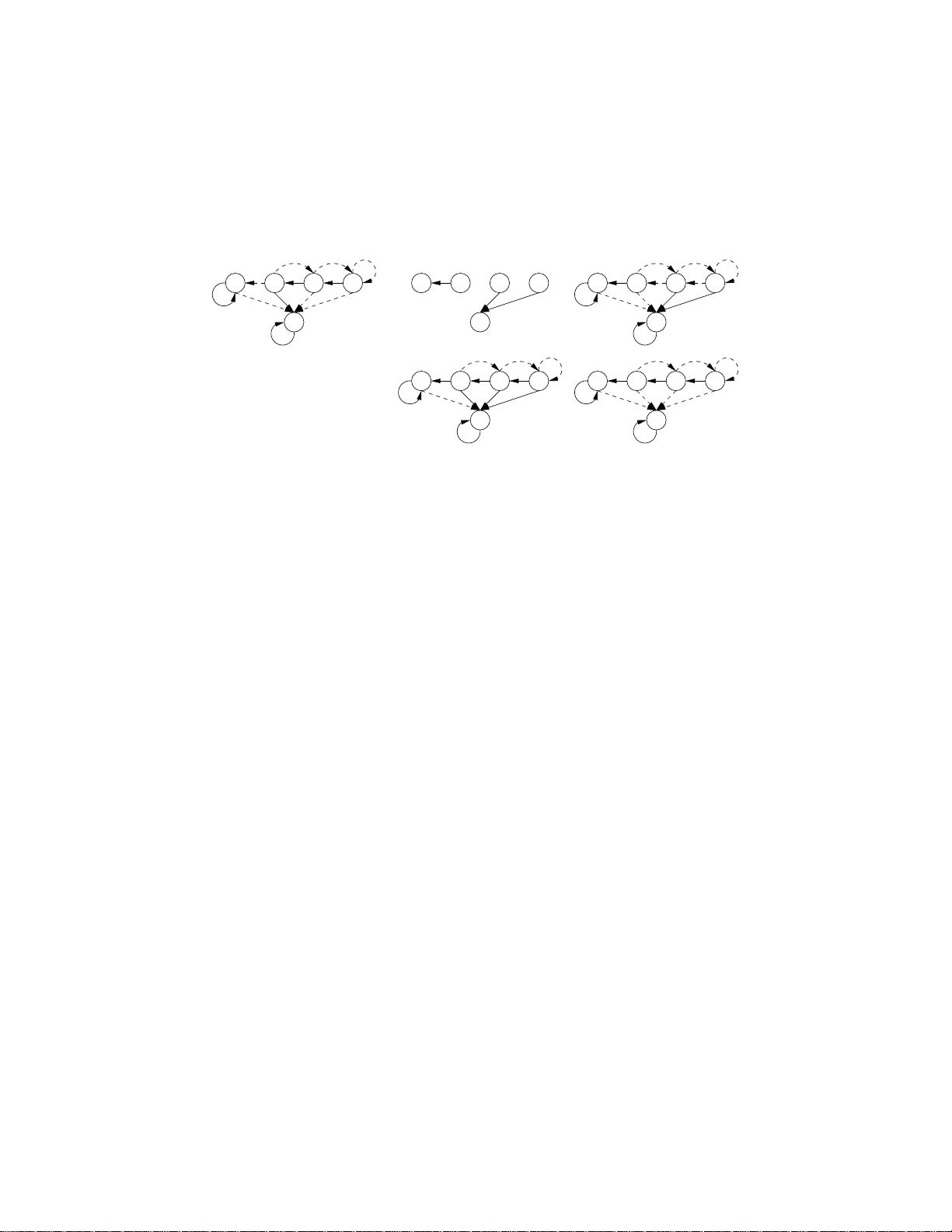
Strategy Iteration using Non-De terministic Strategies for Solvi ng P arity Games Michael Luttenberger ∗ luttenbe@m odel.in.t um.de October 26, 2018 Abstract This article extends the idea of solving parity games by strategy iteration to non-deterministic strategies: In a n on-deterministic strategy a player restricts him- self to some non-empty subset of possible actions at a giv en node, instead of lim- iting himself to exactly one action. W e sho w that a strategy-improv ement algorithm by by Bj ¨ orklund, Sandber g, and V orobyo v [3] can easily b e ada pted to the more general setting of non-deterministic strategies. Further, we sho w that ap plying the heuristic of “all profitable switches” (cf. [1]) leads t o choosing a “locally optimal” successor strategy in the setting of non-deterministic strategies, thereby obtaining an easy proof of an algorithm by Sche we [13]. In contrast to [3], we present our algorithm directly for parity games which allows us to comp are it to the algo rithm by Jurdzinsk i and V ¨ oge [15]: W e s how that the v aluations used in both algorithm coinc ide on parity gam e arenas in which on e player can “surrender”. Thus, our algorithm can al so be seen as a generalization of the one by Jurdzinski and V ¨ oge to non-deterministic strategies. Finally , usin g non -deterministic strategies allows us to sho w that the nu mber of improv ement steps is bound fro m abo ve by O (1 . 724 n ) . For strategy-impro vement algorithms, this bound was pre viously only kno wn to be attainable by using ran- domization (cf. [1]). 1 Introd uction A parity game arena consists of a directed graph G = ( V , E ) where e very vertex belongs to exactly o ne of tw o players, called player 0 and player 1 . Every vertex is colored by some natural number in { 0 , 1 , . . . , d − 1 } . Starting from som e initial v ertex v 0 , a play of both play ers is an in finite p ath in G where th e owner of the curren t node determines the next vertex. In a parity game, the winner of such an infinite play is then defined by th e parity of the maxima l color which a ppears infinitely often along the giv en play . ∗ Institut f ¨ ur Informatik, T echnische Univ ersit ¨ at M ¨ unchen 1 As shown b y Mostowski [ 11], and independ ently by Em erson and Jutla [4], there exists a partitio n of V in two sets W 0 and W 1 such that player i h as a m emory less strategy , i.e. a m ap σ i : V i → V which maps every vertex v co ntrolled by p layer i to some successor v , so that play er i wins a ny play starting from som e w ∈ W i by using σ i to determine his moves. Interest in p arity games arises as d etermining the winn ing set W 0 is equivalent to deciding wheth er a given µ -c alculus for mula holds w .r .t. to a given Kripke struc ture, i.e. determ ining W 0 is equivalent to the mod el checking prob lem of µ -calculus. Further interest is sparked as it is k nown that solvin g parity games is in UP ∩ co-UP [8], but no polyno mial time algorithm has been foun d yet. In th is article we consider an approach for calculating the winning sets which is known as strategy iter ation or strategy improvement, an d can be de scribed a s follows in the setting of g ames: In a first step, a way for valuating the strategies of p layer 0 is fixed, thereby inducing a partial o rder on the strategies of pla yer 0 . Then , one chooses an in itial strategy σ : V 0 → V fo r p layer 0 . Iter ativ ely (i) the c urrent strategy is valu- ated, ( ii) b y m eans o f th is valuation p ossible im provements of th e cu rrent strategy are determined , i.e. pa irs ( u, v ) such that σ [ u 7→ v ] is a stra tegy having a b etter valuation than σ , (iii) a subset of the possible improvements is selected a nd im plemented yield - ing a better strategy σ ′ : V 0 → V . These steps are repeated until n o improvements can be found anymore. Although this approac h usually (using n o rand omization [1]) allows only to g iv e a bound exponential in | V 0 | on th e number o f iterations n eeded till termination, there is no family o f games kn own for which this approach leads to a super-polynomial n umber of improvement steps. It is th us also used in practice e.g. in com pilers [14]. In p articular, th is appr oach has been successfu lly applied in several d ifferent sce- narios like M arkov decision pro cesses [ 6], stocha stic g ames [5], or discoun ted payo ff games [12]. Using reduction s, these algor ithms can also be used for solvin g parity games. In 200 0 Jurdzinski an d V ¨ oge [1 5] presen ted the first strategy-improvement algorithm fo r p arity game s which directly work s on the g iv en par ity game with out r e- quiring a ny redu ctions to some in termediate rep resentation. Alt hou gh the algorithm by Jur dzinski an d V ¨ oge did not lead to a better upper bound o n the co mplexity of de- ciding the win ner of a parity game with n nodes and d colo rs (the algor ithm in [15] has a c omplexity of O (( n/d ) d ) whereas th e uppe r bound of O (( n/d ) d/ 2 ) was already known at that t ime [9]), it sparked a lot of interest as the strategy -improvement process w .r .t. parity games is directly observable and not obfu scated by some reduction. In th is article, we extend strategy iteration to non-deterministic str ategies : In a non- deterministic strategy a p layer is no t req uired to fix a single suc cessor f or any vertex controlled by him instead he restricts him self to s ome non-e mpty subset of all possible successors. Using no n-deter ministic strategies seems to be more natu ral, as it allows a player to on ly “disable” tho se moves along which the valuation of the current strategy decreases. Our algorithm is an extension of an algo rithm by Bj ¨ orklun d, Sandberg, and V oroby ov [3] proposed in 2004. In p articular, we borrow their idea of giving one o f the two pla yers the option to give u p and “escape” an infin ite play he would lose by introdu cing a sink. In con trast to th e origin al algo rithm in [3] we present this extended algorithm directly for parity gam es in order to b e able to comp are this algorithm d irectly with the one by Ju rdzinski and V ¨ oge, and also in the hope tha t th is 2 might lead to better insights regarding the s trategy improvement p rocess. Strategy iteration, as described above, chooses in step (iii) some subset of possible changes in or der to obtain the next (deterministic) strategy . A natural qu estion is how to choo se th is set of ch anges. Obviously , on e would like to choose these sets in such a way that the total number o f improvements steps is as small as possible – we call this “globally optimal”. A s no efficient algorithm for deter mining these sets is kn own, usually heu ristics are u sed instead . One h euristic applied qu ite often in the case of a binary arena is c alled “all p rofitable switches” [1]: In a binar y ar ena, given a strategy σ : V 0 → V we can refer to th e successors of v ∈ V 0 by σ ( v ) and σ ( v ) . A strategy improvement step then amoun ts to d eciding f or ev ery node v ∈ V 0 whether to switch from σ ( v ) to σ ( v ) , or not. “ All possible switches” r efers th en to the heur istic of switch- ing to σ ( v ) of ev ery v ∈ V if this switch is a n improvement w .r .t. the used valuation. T ransferr ing th is heur istic to the setting of no n-determ inistic strategies the heu ristic becomes simply t o choo se th e set of all possible improvements of the gi ven strategy as the new strategy con sidered in th e next step. W e show that this simple heuristic lead s to the “locally optimal” improvement, i.e. the strategy which is at least as good as any other strategy ob tainable by im plementing a su bset of the possible improvements. By applyin g th is heur istic in ev ery step we o btain a n ew , in our opinio n m ore natural and accessible, presentation of the algorithm b y Schewe pro posed in [ 13]: There only valuations (referred to a s “estimation s” there), a nd d eterministic strategies are consid- ered, whereas the strategy impr ovement process itself, and the connection to [3] ar e obfuscated . Fur ther, the a lgorithm in [13] d oes not work directly on par ity games, and requires some u nnecessary restrictions on the g raph structure o f the ar ena, e .g. only bipartite arenas are considered. W e then com pare our alg orithm using non-determ inistic strategies to the one by Jurdzinski an d V ¨ oge [15]. This is not possible w .r .t. the algorithm in [3] o r [1 3] as these do not work directly on parity games. Here, we can show that the v aluation used in o ur algorithm , resp. in [15] coincide, w hich read ily allows us to conc lude that th e locally optimal improvement o btained by our algor ithm is always at least as good as any locally improvement obtain able by [15]. W e obtain an u pper bou nd of O ( | V | 2 · | E | · ( | V | d + 1) d ) f or ou r algorith m which is the same as the one obtainable when using deterministic strategies [3] . So usin g non-d eterministic strategies come s “for free”. Of course, w .r .t. to th e sub-exponen tial bound of | V | O ( √ | V | ) obtainable fo r the algo rithm by Jurdzin ski, Paterson and Zwick [7], our algorithm is not competitive. Still, we think that our algorithm is inter esting as strategy-iteration in practice only requires a poly nomial number of improvement s teps in gen eral, as already mentioned above. In p articular, we ca n show that the number of impr ovement step s done b y our alg orithm when using the “all p rofitable switches”- heuristic, and thus by the on e by Schewe [13], is b ound ed by O (1 . 72 4 | V 0 | ) , wh ereas th e best known up per bound for strategy iteration when using only deterministic strategies and no ran domizatio n in the im provement selectio n is O (2 | V 0 | / | V 0 | ) [1]. I n particular, the bo und o f O (1 . 724 | V 0 | ) was pr eviously known to be obtainable only b e choosing the improvements r andomly [1]. 3 Organization: Section 2 summarizes the standard definitions and results regar ding parity games. In Section 3 we extend parity games by allowing player 0 to terminate infinite plays in order to escap e an infin ite play he would lose. This idea was first stated in [ 3]. W e combine this with a gen eralization of the path profiles used in [15] in orde r to get an alg orithm working directly on par ity games. Section 4 summ arizes our strategy improvement algorithm using non -determin istic strategies. Section 5 th en compare s t he algor ithm presented in this article with the one by Jurdzinski and V ¨ oge. 2 Pr eliminaries In this section w e repeat the standard definitions and notations regard ing parity games. An arena A is g iv en by ( V , E , o ) , if ( V , E ) is a finite, d irected grap h, where o : V → { 0 , 1 } assigns each node an owner . W e denote by V i := o − 1 ( i ) the set of all nodes belonging to player i ∈ { 0 , 1 } , an d write E i for E ∩ V i × V . Given some subset V ′ ⊆ V we write A| V ′ for the restriction of the arena A to the nod es V ′ . A play π ∈ V N ∪ V ∗ in A is any maximal p ath in A where we assume that play er i determines the move ( π ( i ) , π ( i + 1)) , if π ( i ) ∈ V i . For ( V , E ) a directed graph, and s ∈ V a node we write sE for the set of succe ssors of s . For A = ( V , E , o ) an arena, a (mem oryless) str ategy of player i (sho rt: i - strate gy) ( i ∈ { 0 , 1 } ) is any subset σ ⊆ E i satisfying ∀ s ∈ V i : | sE | > 0 ⇒ | sσ | > 0 , i.e. a strategy d oes not intro duce a ny n ew dead end s. σ is d eterministic , if | sσ | ≤ 1 for all s ∈ V i . W e write E σ for E σ = E 1 − i ∪ σ , and A| σ for ( V , E σ , o ) . W e assume that th e reader is familiar with the concep t of attractors. For con ve- nience, a definition can be found in the append ix. A p arity game ar ena A is gi ven by ( V , E , o, c ) where ( V , E , o ) is an ar ena with v E 6 = ∅ for all v ∈ V , and c : V → { 0 , 1 , . . . , d − 1 } assigns each n ode a color . The winner of a p lay π in a parity game arena is gi ven by lim sup i ∈ N c ( π ( i )) (mo d 2) . Giv en a node s , a strategy σ ∈ E i is a winning strategy fo r s o f p layer i , if h e wins any play in A| σ starting fro m s . Player i wins a n ode s , if he ha s a winning strategy for it. W i denotes the set o f no des won by player i . As we assume that every node has at least one successor, there are only in finite p lays in a par ity ga me arena . Wlog., we fu rther assume that c − 1 ( k ) 6 = ∅ for all k ∈ { 0 , 1 , . . . , d − 1 } as we may o therwise reduce d . A cycle s 0 s 1 . . . s n − 1 (with s i +1 (mo d n ) ∈ s i E ) in a parity game arena A is called i -dominated , if the parity of its highest color is i . Player i wins the node s using strategy σ ⊆ V i × V , iff e very cycle reachable from s in A| σ is i -d ominated. Theorem 2.1. [11, 4] For any a parity g ame arena A we have W 0 ∪ W 1 = V . Player i possesses a deterministic strategy σ ∗ i : V i → V with which he win ev ery node s ∈ W i . 3 Escape Aren as In this sectio n we extend parity games b y allowing player 0 to escape an in finite play which he would loose w . r .t. the parity game winning condition: 4 Let A = ( V , E , o ) be a parity g ame arena. W e ob tain the ar ena A ⊥ = ( V ⊥ , E ⊥ , o ⊥ ) from A by introd ucing a sink ⊥ V ⊥ := V ⊎ { ⊥} where only player 0 can ch oose to p lay to ⊥ ( E ⊥ := E ∪ V 0 × {⊥} ). Th e sink ⊥ itself has no ou t-going edges, and we assume that p layer 0 contro ls ⊥ ( o ⊥ := o ∪ { ( ⊥ , 0) } althou gh this is of no real impor tance. Although , this construction was first p roposed in [3] we refer to A ⊥ as escape arena in the style of [ 13]. As A ⊥ itself is n o par ity game arena anymo re, we hav e to d efine the winner o f such a finite play as we ll. For this we extend the definition of c olor p r ofi le , which was first stated in [2], to finite plays: For a given escape are na A ⊥ using d colors { 0 , 1 , . . . , d − 1 } , we define th e set P of color pr ofiles by P := Z d ∪ {−∞ , ∞} where Z d is the set of d -dimensional integer vector s. W e wr ite ø for the zero- profile (0 , 0 , . . . , 0) ∈ Z d , and u se standard addition on Z d for two p rofiles ℘, ℘ ′ ∈ Z d . The idea of a pr ofile ℘ ∈ P is to co unt how o ften a gi ven color appears a long a fi nite play , wh ereas −∞ , reps. ∞ correspo nd to infin ite play s won by p layer 1 , r esp. p layer 0 . Mo re precisely , f or a finite sequence π = s 0 s 1 . . . s l of vertices, th e value ℘ ( π ) of π is the profile which counts how often a colo r k ∈ { 0 , 1 , . . . , d − 1 } ap pears in c ( s 0 ) c ( s 1 ) . . . c ( s l ) . For an infinite sequence π = s 0 s 1 . . . , its va lue ℘ ( π ) is defined to be ∞ , if π is w on by player 0 w .r .t. the parity game win ning condition ; o therwise ℘ ( π ) := − ∞ . Finally , we in troduce a total order ≺ on P wh ich tries to capture the notion of wh en one of two gi ven plays is better than the other for player 0 : For this we set (i) − ∞ to be the bottom elemen t of ≺ , (ii) ∞ to be the top element of ≺ , and (iii) for all ℘, ℘ ′ ∈ P \ {−∞ , ∞} we set: ℘ ≺ ℘ ′ : ⇔ ∃ k ∈ { 0 , 1 , . . . , d − 1 } : k = ma x { k ∈ { 0 , 1 , . . . , d − 1 } | ℘ k 6 = ℘ ′ k } ∧ ( k ≡ 2 0 ∧ ℘ k < ℘ ′ k ∨ k ≡ 2 1 ∧ ℘ k > ℘ ′ k ) . Inform ally , th e definition of ≺ says that play er 0 hates to loose in an infinite pla y , whereas he likes it the m ost to win an infinite play . So, whenev er he can, he w ill try to escape an in finite p lay he cann ot win , there fore resu lting in a finite p lay to ⊥ : here, given two finite plays π 1 , π 2 ending in ⊥ , play er 0 looks for the highest colo r c which does n ot appear equally often alon g both plays. If c is even, he p refers that play in wh ich it ap pears more o ften; if it is o dd, he p refers the on e in wh ich it app ears less o ften. In par ticular, player 0 dislikes visiting o dd-do minated cycle, while he likes visiting ev en-d ominated o nes: Lemma 3.1. Assume that χ = s 0 s 1 . . . s n is a non-empty c ycle in the parity game are na A , i.e. s 0 ∈ s n E and n ≥ 0 . χ is 0 - domina ted, i.e. the hig hest co lor in χ is e ven if and on ly if ℘ ( χ ) ≻ ø. χ is 1 -do minated if and only if ℘ ( χ ) ≺ ø. Now , fo r a g iv en parity g ame aren a A let σ ∗ 0 , σ ∗ 1 be the optimal winning strategies of p layer 0 , resp. 1 . Furth er , let W 0 , W 1 be the correspond ing winning sets. Obvio usly , both players can still use these strategies in A ⊥ , too, as we only added add itional edges. Especially , player 0 ca n still use σ ∗ 0 to win W 0 in A ⊥ as only he has the option to move to ⊥ . In the c ase o f player 1 , by applying σ ∗ 1 any cycle in A ⊥ | σ ∗ 1 reachable from a vertex v ∈ W 1 has to be odd -dom inated. Hence , player 0 prefer s to play in an acyclic path from v to ⊥ in A ⊥ | σ 1 when starting from a vertex in W 1 . Let ther efore be ℘ the ≺ - maximal value of any acyclic p ath termina ting in ⊥ in A ⊥ . ℘ is the best p layer 0 can h ope to achieve startin g fro m a n ode v ∈ W 1 when player 5 1 plays o ptimal. W e ther efore d efine: player 0 wins a play π , if ℘ ( π ) ≻ ℘ , oth erwise player 1 w ins the play . Play er i wins a node s ∈ V , if h e has a strategy σ ⊆ E i with which he wins any play startin g from s in A| σ . As already sketched, this leads then to the following th eorem. Theorem 3.2. Player i wins the node s in A iff he wins it in A ⊥ . 4 Strategy Improv ement W e now tu rn to the prob lem of findin g o ptimal winning strategies b y iterativ ely valu- ating the stra tegy , and deter mining from th is valuation p ossible better stra tegies. The following section can be seen as the gene ralization o f the algo rithm in [3] to non- deterministic strategies and explicitly stated in the setting of p arity g ames. In fact, we will o nly co nsider a special class of strategies for player 0 , i.e. suc h strategies wh ich do not intro duce any 1 -dom inated cycles. The strategy im provement pr ocess will assure that no 1 -dom inated c ycles ar e created. If th ere are any 1 -domin ated cycles in A ⊥ | V 1 , then playe r 1 wins all the n odes in the 1 -attractor to these cycles. W e may , thus, identify the nodes tri vially won by player 1 in a preprocessing step, and remove the m. Assumption 4.1. The arena A ⊥ | V 1 has no 1 -domin ated c ycles. Definition 4.2. W e call a strategy σ ⊆ E 0 of player 0 r easona ble , if the re are no 1 -domin ated cycles in A ⊥ | σ . Remark 4.3. (a) By our assum ption above the strategy σ ⊥ := V 0 × { ⊥} is re asonable, as every 1 -dom inated cycle in A consists of at least one nod e co ntrolled b y player 0 . ( b) Let σ be any strategy of p layer 0 , and W σ the set of no des won by σ . Then, the strategy σ ′ = σ ∩ ( W σ × W σ ) ∪ { ( s, ⊥ ) | s ∈ V 0 \ W σ } is reasonable with W σ = W σ ′ . W e m ay thus assume that player 0 uses o nly reasonab le stra tegies. Definition 4.4. Let σ be some reason able strategy of player 0 . Its valuation V σ : V ∪ { ⊥} → P m aps ev ery node s on the ≺ -minim al value V σ ( s ) which player 1 can gua rantee to achieve in any play starting from s in A ⊥ | σ by using some memoryless strategy: V σ ( s ) := ≺ min τ ⊆ E 1 strategy ≺ max { ℘ ( π ) | π is a play in A ⊥ | σ,τ ∧ π (0) = s } , where we set V σ ( ⊥ ) := ø . Remark 4.5. (a) W e will show later that, if we start fr om th e r easonable stra tegy σ ⊥ := V 0 × {⊥} , then our strategy-improvement algorithm will only generate reaso nable strategies. (Note, if A ⊥ | σ ⊥ had 1 -domina ted cycles, then these would need to exist solely in A| V 1 – but we have assumed above that we r emoved those in a p repro cessing step.) (b) As 6 shown above, for all s ∈ W 1 player 1 can use his op timal winning s trategy σ ∗ 1 from the parity game to guarantee V σ ( s )  ℘ ≺ ∞ . By m eans of the valuation V σ we can partially ord er r easonable strategies in the natural way: Definition 4.6. For two (r easonable) strategies σ a , σ b of p layer 0 we write σ a  σ b , if V σ a ( s )  V σ b ( s ) for a ll nodes s . W e write σ a ≺ σ b , if there is at least one n ode s such that V σ a ( s ) ≺ V σ b ( s ) . Finally , σ a ≈ σ b , if σ a  σ b ∧ σ b  σ a . The f ollowing lemma ad dresses the calculation of V σ using a straight-forward adaption of the Bellman-Ford algorithm: Lemma 4.7. Let σ ⊆ E 0 be a reason able strategy of player 0 . W e define V ⊥ : V ∪ { ⊥ } → P by V ⊥ ( ⊥ ) := ø, and V ⊥ ( s ) = ∞ f or all s ∈ V , and the op erator F σ : ( V ∪ { ⊥} → P ) → ( V ∪ {⊥} → P ) by F σ [ V ]( ⊥ ) := ø F σ [ V ]( s ) := ℘ ( s ) + min  {V ( t ) | ( s, t ) ∈ E 1 } if s ∈ V 1 , F σ [ V ]( s ) := ℘ ( s ) + max  {V ( t ) | ( s, t ) ∈ σ } if s ∈ V 0 , for any V : V ∪ {⊥} → P . Then, the valuation V σ of σ is g iv en as th e limit of the sequence F i σ [ V ⊥ ] for i → ∞ , and this limit is reached after at most | V | iteratio ns. Remark 4.8. (a) W e a ssume unit cost fo r adding and com paring color profiles. The tim e needed for calculating V σ is then simply giv en by O ( | V | · | E | ) . (b) For every s ∈ V there has to be at least one edge ( s, t ) with V σ ( s ) = ℘ ( s ) + V σ ( t ) , as V σ = F σ [ V σ ] . W .r .t. V σ we can identify possible impr ovements of σ : Definition 4.9. Let σ ⊆ E 0 be a reasonable strategy o f player 0 . The set I σ of impr ovements , resp. the set S σ of strict impr ovements of σ is defin ed by • I σ := { ( s, t ) ∈ E 0 | V σ ( s )  ℘ ( s ) + V σ ( t ) } , resp. • S σ := { ( s, t ) ∈ E 0 | V σ ( s ) ≺ ℘ ( s ) + V σ ( t ) } . W e call a strategy σ ′ ⊆ E 0 a dir ect impr ovemen t of σ if σ ′ ⊆ I σ . Fact 4.10. Let σ ′ be a dire ct imp rovement of σ . Then alo ng every edge ( u , v ) of A ⊥ | σ ′ we h ave V σ ( u )  ℘ ( u ) + V σ ( v ) . In particular, we hav e for any fin ite path s 0 s 1 . . . s l +1 in A ⊥ | σ ′ V σ ( s 0 )  ℘ ( s 0 ) + V σ ( s 1 )  ℘ ( s 0 s 1 ) + V σ ( s 2 )  . . .  ℘ ( s 0 . . . s l ) + V σ ( s l +1 ) . From this easy fact, se veral important properties of direct improvements fo llow: Corollary 4.11. If σ is reasonable, then any 0 -strategy σ ′ ⊆ I σ is reasonable, too. 7 Corollary 4.12. Let σ be a reasonable strategy . For a direct impr ovement σ ′ of σ we h av e that σ  σ ′ . If σ ′ contains at least on e strict imp rovement of σ , then this inequality is strict, i.e. σ ≺ σ ′ . The p receding corollar ies show that starting with an in itial reaso nable strategy σ 0 , e.g. σ ⊥ , we can ge nerate a sequen ce σ 0 , σ 1 , σ 2 , . . . of reaso nable strategies such that V σ i ( s )  V σ i +1 ( s ) for all s ∈ V , if we choose the strategy σ i +1 to be some d irect improvement o f σ i . Further, we know , if σ i +1 uses at least o ne strict improvement ( s, t ) of σ i , i.e. ( s, t ) ∈ σ i +1 ∩ S σ i 6 = ∅ , then we have V σ i ( s ) ≺ V σ i +1 ( s ) , i.e. ev ery possible reasonable strategy occur s at most o nce along th e strategy improvemen t seq uence. As already sh own, we h av e a lw ays V σ i ( s )  ℘ ≺ ∞ for all n odes s ∈ W 1 . Th e obvio us question is now , if we can reach an optimal winning strategy by th is procedure, i.e. is a reasonable strategy σ with S σ = ∅ o ptimal? Th is is answered in the following le mma. Lemma 4.13. As long as there is a node s ∈ W 0 with V σ ( s ) ≺ ∞ , σ has at least on e strict improve- ment. Due to this lemma, we know that, if a reasonable strategy σ has no strict improve- ments, i.e. S σ = ∅ , then we h ave V σ ( s ) = ∞ for at least all the nod es s ∈ W 0 . On th e other h and, fo r all nod es s ∈ W 1 we a lways have V σ ( s )  ℘ . Hence, by the determi- nacy of parity gam es, i.e. W 1 = V \ W 0 , σ ha s to be a n o ptimal winnin g strategy fo r player 0 , if S σ = ∅ . By our constructio n such an optim al stra tegy σ with S σ = ∅ might be non-d eterministic. The f ollowing lem ma shows how one can dedu ce an o ptimal deterministic strategy from such a σ . Lemma 4.14. Let σ be a reasonable strategy of player 0 in A ⊥ , and I σ the strate gy co nsisting o f all impr ovements of σ . Then every deterministic strategy σ ′ ⊆ I σ with V I σ ( s ) = ℘ ( s ) + V I σ ( t ) for all ( s, t ) ∈ σ ′ satisfies V I σ = V σ ′ . Starting fro m σ ⊥ = { ( s, ⊥ ) | s ∈ V 0 } , if we improve the curren t stra tegy using at least one strict improvement in ev ery step, we will end up with an optimal winning strategy for player 0 . As in every step th e valuation increases in at least those n odes at which a strict improvement exists, and as there are at mo st ( | V | d + 1) d possible values a v aluation can assign a giv en node, the num ber of improvement steps is bo und by | V | · ( | V | d + 1) d . The cost of e very improvement step is g iv en by the cost of the calculation of V σ , we thus get: Theorem 4.15. Let σ 0 be some reasonable 0 -strategy . By iteratively taking σ i +1 to be some direct improvement of σ i which uses at least one strict improvement, one obtains an op timal winning s trategy after at most | V | · ( | V | d + 1) d iterations. Th e total running time is thus O ( | V | 2 · | E | · ( | V | d + 1) d ) . 8 4.1 All Pr ofitable Switches In the p revious subsection we have not said anythin g about which d irect impr ovement should be taken in every improvement step. As no algorith ms are known which d e- termine for a given strategy such a direct improvement that the total n umber of im - provement steps is minimal ( we call su ch a direct improvement “glo bally optima l”), one usual resorts to he uristics for ch oosing a dir ect improvement, (see e.g. [1]).Most often the h euristic “all pro fitable switches” mentio ned in the introdu ction is used. In the case o f non -determin istic strategies this simply becom es taking I σ as successor strategy . The in teresting fact here is that I σ is a “locally optimal” d irect im provement for a given reasonable strategy σ , i.e. for all strategies σ ′ ⊆ I σ we h ave σ ′  I σ . W e remark that this has already been shown implicitly by Schewe in [13]: Theorem 4.16. Let σ be a reaso nable strategy with I σ its set of improvements. For any direct improve- ment of σ we hav e σ ′  I σ . W e like to gi ve an e asy proof fo r this theorem. W e first note the following two proper ties o f the operato r F σ : Fact 4.17. (i) For V , V ′ : V ∪ {⊥ } → P with V  V ′ we have F σ [ V ]  F σ [ V ′ ] . (ii) For tw o 0 -strategies σ a ⊆ σ b we have F σ a [ V ]( s )  F σ b [ V ]( s ) for all s ∈ V . Using (i) and (ii) we get by inductio n F i +1 σ a [ V ⊥ ] = F σ a [ F i σ a [ V ⊥ ]]  F σ a [ F i σ b [ V ⊥ ]]  F σ b [ F i σ b [ V ⊥ ]] = F i +1 σ b [ V ⊥ ] , and therefore the following lemma: Lemma 4.18. If σ a and σ b are reasonable and σ a ⊆ σ b , it holds that V σ a  V σ b . Now , as the set of improvements I σ of a gi ven reasonable strategy σ is itself a (non- deterministic) strategy , an d every direct imp rovement σ ′ of σ satisfies σ ′ ⊆ I σ by defin ition, the the orem fr om above follows. T he a lgorithm of Schewe in [13] can therefor e be described as an op timized implem entation of non-determin istic strategy iteration using the “all profitable switches” heuristic. W e close this section with a remark on the calculation of V I σ . Schewe pr oposes an algorithm for calculating V I σ which uses V σ to speed u p the calculation lead- ing to O ( | E | lo g | V | ) op erations on color -pr ofiles in stead of O ( | E | · | V | ) . F or this, formu lated in the notation of our algorithm, he introduces edge weights w ( u, v ) := ( ℘ ( u ) + V σ ( v )) − V σ ( u ) , and calculates w .r .t. these edges an update δ = V I σ − V σ . W e argue that one can use Dijkstra’ s algorithm for this, as we ha ve V σ ( u )  ℘ ( u ) + V σ ( v ) along all ed ges ( u, v ) ∈ I σ , and thus w ( u, v )  ø , i.e. a ll edg e weights are n on- negativ e. Proposition 4.19. V I σ can b e calculated u sing Dijkstra’ s a lgorithm which need s O ( | V | 2 ) o peration s on color-profiles on dense graph s; for grap hs whose out-degre e is bo und b y so me b th is 9 can be improved to O ( b · | V | · log | V | ) by using a heap 1 . This gives us a r unning time of O ( | V | 3 · ( | V | d + 1) d ) , r esp. O ( | V | 2 · b · log | V | · ( | V | d + 1) d ) . 5 Comparison with the Algorithm by Jurd zinski and V ¨ oge This section compares the algorithm presen ted in this article with the on e by Jurdzinski and V ¨ oge [15]. W e fir st give a short (slightly imprecise) descriptio n of the alg orithm in [15]: This algor ithm starts in each step with some deterministic 0 - strategy σ . Using σ a v aluation Ω σ is calculated (see below for details about Ω σ ). T hen, by means o f t his valuation possible strate gy improvements are determined, and finally some non -empty subset of these imp rovements is chosen, but only on e improvement per no de at most, such that implemen ting these imp rovements yields a deterministic s trategy again. This process is r epeated until there are no imp rovements anymore w .r .t. the current strategy . The valuation Ω σ : W e present a slightly “op timized” version o f the valuation u sed in [1 5]. The valuation Ω σ ( s ) o f a determ inistic 0 -strategy σ consists of the the cycle value z σ ( s ) , the path pr o file ℘ σ ( s ) , and the path length l σ ( s ) which are define d as follows: • As σ is determin istic, all p lays in A| σ are determined by player 1 . For e very node z having od d co lor, we can decide wheth er th ere is at least one cycle in A| σ such that th is cycle is dominated by z . Le t Z be th e set of all o dd colored nod es dominatin g a cycle in A| σ . Giv en a nod e s we de fine z σ ( s ) to b e a no de o f maximal color in Z , which is reachable f rom s in A| σ ; if no n ode in Z is r eachable f rom s in A| σ , th en s has to be won by player 0 , and we set z σ ( s ) = ∞ . • If z σ ( s ) is some odd colored node , the second com ponent ℘ σ ( s ) be comes th e color p rofile of a ≺ -minima l p lay from s to z σ ( s ) in A| σ – with the restriction that only nodes of color ≥ c ( z σ ( s )) are counted. • Finally , if ℘ σ ( s ) is d efined, l σ ( s ) is th e leng th of shorte st play fro m s to z σ ( s ) w .r .t. ℘ σ ( s ) , if z σ ( s ) has odd color . Remark 5.1. W e a ssume here th at z σ is either ∞ , if s is alr eady won using σ , or the “worst” odd - dominated cycle into wh ich player 1 can f orce a p lay starting f rom s . In [ 15], the authors even try to o ptimize z σ ( s ) wh en s is already won using σ . These impr ovements are obviou sly unnecessary , as we ca n always rem ove the attractor to these n odes fro m the arena in an intermediate step in order to obtain a smaller arena. 1 In [3] the authors propose another optimizat ion to speed up the calculati on of V σ by restrictin g the re- calcu lation of V σ to only those nodes where V σ change s. Those nod es can be easi ly identified by calculati ng an attractor again in time O ( | E | ) . Unfortuna tely , combining t his optimiz ation with the one by Sche we ([13]) does not lead to a bett er asymptotic upper bound. 10 Further, it is assumed in [15] that e very n ode is uniquely colored. T herefor e, in [15] ℘ σ is defined to be the set of nodes having higher color than z σ ( s ) on a “worst” path from s to z σ ( s ) . Jurdzinski and V ¨ oge already mention at the end of [15] that their algorithm also works when not assum ing that ev ery vertex is un iquely color ed, but do not present the adapted data stru ctures needed in this case. This was done in [2]: If the same colo r is used for se veral vertices, it is sufficient to only count the number of no des having a color k ≥ z σ ( s ) alo ng such a “worst” path from s to z σ ( s ) wh ere “worst” path simply mean s a ≺ -minimal path then. Theref ore, the c olor pr ofiles used in this article are a direct generalization of the path profiles used in [15]. In [15] an ed ge ( s, t ) ∈ E 0 is now called a strict imp rovement over ( s, σ ( s )) , if Ω σ ( t ) is strictly better than Ω σ ( σ ( s )) , i.e. either the “worst” cycle imp roves, or the worst play to it im proves, or the length of a worst play bec omes longer (“the lon ger player 0 can stay away from z σ the better for him”). A d eterministic strategy σ ′ is then a direct improvement of a giv en determ inistic strategy σ w .r .t. [15 ], if it differs fro m σ only in strict improvements. Definition 5.2. For a gi ven parity game arena A = ( V , E , c, o ) , set A ⊥ := ( V ∪ {⊥} , E ∪ V 0 × {⊥} ∪ { ( ⊥ , ⊥ ) } , c ∪ { ( ⊥ , − 1) } , o ∪ { ( ⊥ , 0 ) } ) . A ⊥ results f rom A ⊥ by simply a dding a lo op to ⊥ , and giving ⊥ the color − 1 so that A ⊥ is a p arity gam e arena where ⊥ is the cycle domin ated by the lea st o dd color . A straight- forward ad aption of th e pro of of Th eorem 3.2 shows that player 0 wins a node s in A iff he wins it in A ⊥ . Now , as th e strategy improvement algorithm in [15] tries to play to th e “best” po s- sible cycle, an optimal strategy (obtained by the algorithm ) will always choose to play to ⊥ fr om a no de s , if s cannot be won by player 0 , as every other 1 - domina ted cycle has at least 1 as maximal color . A strategy σ o f player 0 is therefore “reasonab le” w .r .t. to the algorithm by Jur dzinski and V ¨ oge, if ( ⊥ , ⊥ ) is the on ly 1 -dom inated cycle in A ⊥ | σ . Obviously , we now have an on e-to-on e correspo ndence between reasonab le strate- gies σ in A ⊥ , and reasonab le strategies σ in A ⊥ of player 0 : we simply have to remove or ad d the edge ( ⊥ , ⊥ ) to m ove fr om A ⊥ to A ⊥ and v ice versa. W e therefor e may identify these strategies in the follo wing as one strategy . This allows us to co mpare the improvemen t step of the algo rithm presented in th is article with that of [15]. Indeed, as the color of ⊥ is − 1 ( recall that all othe r no des have colors ≥ 0 ), we have ℘ σ ( s ) = V σ ( s ) fo r all nod es with z σ ( s ) = ⊥ , an d V σ ( s ) = ∞ , if z σ ( s ) 6 = ⊥ . This proves the follo wing proposition : Proposition 5.3. Any (deter ministic) d irect improvement σ ′ of σ identified by [15] is a subset of I σ . Therefo re σ ′  I σ . In o ther words, the algor ithm presented here always chooses lo cally a direct im- provement of σ which is at least as goo d as any d eterministic d irect im provement ob- tainable by [15]. I n the appendix , a small example can be found illustrating this. 11 5.1 Bound on the number of Impr ovemen t Steps W e finish this section by giving an u pper bou nd on th e total numb er o f im provement steps when using the “all pr ofitable switches”-h euristic. In the ca se o f an arena with out-degree tw o, one can show that the number of improvement steps done by the algo- rithm in [15] is bound ed by O ( 2 | V 0 | | V 0 | ) (cf. [ 1]). When considering non-determ inistic strategies the heuristic “all profitable switches” naturally generalizes to simp ly taking I σ as successor strategy in every iteration. Here we can show the following upper bound: Theorem 5.4. Let A ⊥ be a escape- parity-g ame arena where every n ode of p layer 0 has at m ost two successor . Then the number of improvement steps needed to reach an optimal winning strategy is b ound by 3 · 1 . 72 4 | V 0 | when using non -determin istic strategy iter ation and the “all profitable switches”-heur istic. Remark 5.5. T o th e b est of o ur kn owledge this is th e best upper bou nd known for any dete rminis- tic strategy-imp rovement algorithm . In [1] a similar boun d is only obtained by using random ization. 6 Conclusions In th e fir st par t of the article, we presen ted an extended version of the algorithm b y [3] wh ich (i) allows the use o f non-de terministic strategies, and (ii) works directly on the given parity gam e are na with out requ iring a reduction to a mea n payoff g ame as an intermediate step. For (ii), we used the path profiles introduced in [15], resp. a generalized version of it called color profiles (see als o [2]) . W e then showed that the heuristic “all profitable switches” in the setting of non- deterministic strategies leads to the locally best direct im provement, an d th erefore to the algorithm presented in [13].W e further identified the fast calculation of the valua- tion propo sed by Schewe as the Dijkstra algor ithm. Finally , we tu rned to the co mparison of the alg orithm presen ted here to the o ne by Jurdzinski and V ¨ oge [15]. As our algorithm works d irectly on parity games in contra st to [3, 13], we could show that the valuations used in both coincide for parity game arenas with escape for play er 0 . W e finished the article by adaptin g r esults from [10] which allowed us to show that using the “all p rofitable switches”-heur istic in the setting of non-determ inistic strategies allo ws to obtain an upper bound of O (1 . 724 | V 0 | ) on the total numb er of improvement steps. This bou nd also car ries over to the alg orithm in [13]. This bound was pre viously only attainable using randomiza tion [1 ]. Refer ences [1] H. Bj ¨ orklun d, S. San dberg, and S. V orobyov . Optimization on completely u ni- modal hypercu bes. T echnical Report 2002 –18, Department o f Inform ation T ech - nology , Up psala Univ ersity , 2002. 12 [2] H. Bj ¨ orklun d, S. San dberg, and S. V orobyov . A discrete subexpo nential algorithm for parity games. In ST ACS’03 , LNCS 2607, pages 663–674. S prin ger, 2003 . [3] H. Bj ¨ orklund , S. Sandberg, and S. V orobyov . A combin atorial strongly sub ex- ponen tial strategy improvement alg orithm for m ean pay off games. In MFCS ’04 , LNCS 3153, pages 673–6 85. Springer, 20 04. [4] E.A. Em erson a nd C.S. Ju tla. T ree au tomata, mu-calculu s and dete rminacy (ex- tended abstract). In FOCS’91 . IEEE Computer Society Press, 1991. [5] A. Hoffman a nd R. Karp. On nonterm inating stoch astic games. Management Science , 12, 1966. [6] Rona ld A. Ho ward. Dy namic progr amming and markov processes. Th e M.I.T . Pr ess , 1960. [7] M. Jur dzi ´ nski, M. Paterson, and U. Zwick. A determin istic subexponential algo- rithm for solving parity games. In SOD A ’06 . A CM/SIAM , 2006. [8] Mar cin Jurdzi ´ nski. Deciding the winner in parity g ames is in UP ∩ co-UP. I nfor- mation Pr ocessing Letters , 68(3 ):119– 124, November 1998. [9] Mar cin Jurdzi ´ nski. Small prog ress measures for solving parity gam es. In ST AC S 2000 , volume 1770 of LNCS , 2000 . [10] Y . M ansour a nd S. Singh . On the complexity o f p olicy iteration. In UAI 199 9 , 1999. [11] A.W . Mostowski. Games with forbidd en p ositions. T ech nical Report 78, Univer - sity of Gda ´ nsk, 1991. [12] Anuj Puri. Theory of Hybrid Systems and Discr ete Event S ystems . PhD th esis, Electronic Research Laboratory , College of Engineering, University of California, Berkley , 1995. [13] Sven Sch ewe. An optimal strategy imp rovement algorithm f or solving p arity games. T ech nical Report 28, Uni versit ¨ at Saarbr ¨ ucken, 2007 . [14] H. Seid l and T . Gawlitza. Prec ise relation al inv a riants through strategy iter ation. In CSL ’0 7 , LNCS, 2007. [15] Jens V ¨ oge and Marcin Jurdzi ´ nski. A discrete strategy improvement alg orithm for solving parity games (Extende d abstract). In CA V’00 , volume 1855 of LNCS , 2000. 13 A Example: Com parison with the Algorithm b y J ur - dzinski and V ¨ oge d) 0 5 3 1 ⊥ c) 0 5 3 1 ⊥ a) 0 5 3 ⊥ 1 b) 0 5 3 1 ⊥ e) 0 5 3 1 ⊥ a) dep icts an arena A ⊥ where bo ld arrows represent the ed ges of a 0 - strategy σ , and dashed arrows re present edges not included in σ . Fu rther, all nod es belong to player 0 , where the numbe rs inside th e no des repr esent the c olors. b) shows the set S σ of strict improvements w .r . t. σ . c) Th e heuristic applied usu ally f or c hoosing a determ inistic direct im provement of σ is to take a m aximal su bset of S σ so th at for ev ery node, for which a strict improvemen t exists, there is exactly one strict improvement cho sen. In this example this leads to the strategy depicte d in c). d) T he alg orithm pr esented in this article, on the other h and, chooses the n on-de terministic strategy I σ = σ ∪ S σ , as shown in d). e) Calcu lating the valuation of both I σ , and the strategy shown in e) shows that both strategy are equ iv alent w .r . t. their valuation (see also lemma 4.14). This means the strategy I σ is already optima l in dif feren ce to c). B Missing Pr oofs B.1 Preliminaries Definition B.1. Giv en an ar ena A = ( V , E , o ) and a target set T ⊆ V of nod es, we define the i - attractor Attr i [ A ]( T ) to T in A by A 0 := T A i +1 := A i ∪ { s ∈ V i | sE ∩ A i 6 = ∅} ∪ { s ∈ V 1 − i | sE ⊆ A i } Attr 0 [ A ]( T ) := S i ≥ 0 A i . The rank r ( s ) ∈ N ∪ { ∞} of a nod e s w . r .t. to Attr 0 [ A ]( T ) is gi ven by min { i ∈ N | s ∈ A i } where we assume that min ∅ = ∞ . A strategy σ ⊆ E i is th en a n i - attractor strategy to T , if f or every ( s, t ) ∈ σ the rank decreases along ( s, t ) as long as s has finite, non -zero rank. 14 Remark B.2. Obviously , p layer i can use any i - attractor strategy to force any play starting f rom a node with finite ra nk into T on an ac yclic path as the rank is strictly decreasing until T is hit. B.2 Parity Game Ar enas with Escape for Player 0 Lemma 3.1. Assume th at χ = s 0 s 1 . . . s n is a non -empty cycle in th e parity game ar ena A , i.e. s 0 ∈ s n E and n ≥ 0 . χ is 0 -domin ated, i.e. the highest color in χ is e ven if and only if ℘ ( χ ) ≻ ø. χ is 1 -domin ated if and only if ℘ ( χ ) ≺ ø. Pr oo f. Wlog . we may assume that s 0 has the do minating color in χ . As all remaining nodes in χ hav e at most co lor c ( s 0 ) , th e co lor p rofile ℘ ( χ ) is 0 for a ll c olors > c ( s 0 ) . Hence, the hig hest color in wh ich ℘ ( χ ) an d ø differ is c ( s ) . If c ( s ) is even, then ℘ ( χ ) ≻ ø b y d efinition, other wise ℘ ( χ ) ≺ ø, as ℘ ( χ ) c ( s 0 ) > 0 . The o ther direction is shown similarly . Theorem 3.2. Player i wins th e node s in A iff h e wins it in A ⊥ . Pr oo f. L et σ ∗ i be the o ptimal, memory less winning strategy in the p arity game A , an d W i the winning set of of player i w .r .t. σ ∗ i . First consider the case s ∈ W 0 . As only play er 0 c an choose to move to ⊥ , any play π in A ⊥ w .r .t. σ ∗ 0 is a play in A , too. He nce, π is infinite, and won by play er 0 w .r .t. the parity game winning condition . Thus, π has the value ∞ . Assume now that s ∈ W 1 . Player 1 can u se h is optimal strategy to fo rce p layer 0 starting f rom s in to a play su ch that e very cycle v isited is 1 -dominated . If player 0 do es not move to ⊥ , the infin ite play a lso exists in the or iginal parity gam e arena, is theref ore won b y player 1 , and, hence, has the value −∞ in the escape g ame. On the other hand, in the e scape p arity game A ⊥ player 0 h as n ow the optio n to escape any suc h infinite play by op ting to termin ate the gam e by moving to ⊥ . Consider therefo re a finite play π = s 0 s 1 . . . s n ⊥ . Assume th at this path is not acyclic. Thus, as we are only countin g how of ten a giv en color app ears along the path, we may split π in to a simple p ath π ′ from s 0 to ⊤ and sev eral cycles χ 1 , . . . , χ l . By using h is winning strategy σ ∗ 1 player 1 can make sure that every such cycle has an o dd color as m aximal color . I t is now easy to see that ℘ ( χ j ) ≺ ø by defin ition of ≺ . Thu s, we ha ve ℘ ( π ) = ℘ ( π ′ ) + ℘ ( χ 1 ) + . . . + ℘ ( χ l ) ≺ ℘ ( π ′ )  ℘. B.3 Strategy Impr ovement Lemma 4.7. Let σ ⊆ E 0 be a reasonable strate gy o f player 0 . W e define V ⊥ : V ∪ {⊥} → P by V ⊥ ( ⊥ ) := ø, and V ⊥ ( s ) = ∞ for all s ∈ V , and th e o perator F σ : ( V ∪ {⊥} → P ) → ( V ∪ {⊥} → P ) by F σ [ V ]( ⊥ ) := ø F σ [ V ]( s ) := ℘ ( s ) + min  {V ( t ) | ( s, t ) ∈ E 1 } if s ∈ V 1 , F σ [ V ]( s ) := ℘ ( s ) + ma x  {V ( t ) | ( s, t ) ∈ σ } if s ∈ V 0 , 15 for any V : V ∪ {⊥} → P . Then, the valuatio n V σ of σ is given as the limit of the seq uence F i σ [ V ⊥ ] fo r i → ∞ , and this limit is r e ached after at most | V | iterations. Pr oo f. For all V , V ′ : V ∪ {⊥} → P with V ( s )  V ′ ( s ) for s ∈ V ∪ {⊥ } we have F σ [ V ]( s )  F σ [ V ′ ]( s ) , to o, i.e. F σ is mono tone. Obvio usly , we have F σ [ V ⊥ ]( s )  V ⊥ ( s ) fo r all s ∈ V ∪ {⊥} . Therefo re, F i σ [ V ⊥ ]( s ) is mo notonica lly d ecreasing fo r i → ∞ . As σ is reasona ble, V σ ( s ) ≻ −∞ , and it can o nly be finite, if s is in the 1 -attractor to ⊥ in A ⊥ | σ . Fu rther, fo r V σ ( s ) ≺ ∞ , V σ ( s ) h as to b e the value of an acyclic pla y π in A ⊥ | σ . One ther efore check s easily th at V σ is a fixed point of F σ ; h ence, by the monoto nicity o f F σ , and V σ  V ⊥ , we have V σ  F i [ V ⊥ ] for all i ∈ N . Let C i be the set of nod es s ∈ V ∪ { ⊥} such that F i σ [ V ⊥ ]( s ) = V σ ( s ) . Obviously , we h ave ⊥ ∈ C i for a ll i ∈ N . A s F i σ [ V ⊥ ] is m onoton ically decreasing, and bound ed from below b y V σ , we have C i ⊆ C i +1 . Define B i to be the b oundar y of C i , i.e. th e set of nod es s ∈ V \ C i with sE ∩ C i 6 = ∅ ∧ sE ∩ V \ C i 6 = ∅ . If B i ⊆ V 0 , th en p layer 0 has a strategy to stay away from ⊥ ∈ C i for every node s ∈ V \ C i . It is easy to see that F i [ V ⊥ ]( s ) = ∞ for all s ∈ V \ C i in this case. Thus, assume B i ∩ V 1 6 = ∅ . As player 1 eventually needs to enter C i in o rder to reach ⊥ , he h as to use an edge f rom a nod e s ′ ∈ V 1 ∩ B i to C i . At least fo r this node s ′ we hav e to hav e s ′ ∈ C i +1 . Hence, we have to ha ve C i = V for some i ≤ | V | , im plying F i +1 σ [ V ⊥ ] = F i σ [ V ⊥ ] . Definition B.3. W e write τ σ ⊆ E 1 for the 1 -strategy c onsisting of the edges ( s, t ) with V σ ( s ) = ℘ ( s ) + V σ ( t ) . Corollary 4.1 1. If σ is r easonab le, then any d ir ect impr ovement σ ′ of σ is r easonab le, too. Pr oo f. For any cycle s 0 s 1 . . . s l with s 0 ∈ s l E σ , we have V σ ( s 0 )  ℘ ( s 0 . . . s l ) + V σ ( s 0 ) , i.e. ø ≺ ℘ ( s 0 . . . s l ) . Corollary 4.12. Let σ be a reasonable s trate gy . (a) F or a dir ect impr ovement σ ′ of σ we h ave that V σ ( s )  V σ ′ ( s ) for all s ∈ V . (b) If ( s, t ) ∈ σ ′ is a strict impr ovemen t of σ , th en V σ ( s ) ≺ V σ ′ ( s ) . Pr oo f. ( a) Le t s be any node. For any play π = s 0 s 1 . . . s n ⊥ starting from s in A ⊥ | σ we hav e already shown: V σ ( s )  ℘ ( π ) + V σ ( ⊥ ) = ℘ ( π )  V σ ′ ( s ) . 16 (b) As ( s, t ) is a strict improvement of σ , we hav e (i) V σ ( s ) ≺ ℘ ( s ) + V σ ( t ) , ( ii) s ∈ V 0 , and, hence, (iii) V σ ′ ( s ) = ma x ≺ { ℘ ( s ) + V σ ′ ( t ′ ) | ( s, t ′ ) ∈ σ ′ } . With the result from (a) it follows th at V σ ( s ) ≺ ℘ ( s ) + V σ ( t )  ℘ ( s ) + V σ ′ ( t )  V σ ′ ( s ) . Lemma 4.13. As lon g as ther e is a node s ∈ W 0 with V σ ( s ) ≺ ∞ , σ h as at least one strict impr ovement. Pr oo f. L et A be the set o f nod es t with V σ ( t ) ≺ ∞ , i.e. A is the 1 -attr actor to ⊥ in A ⊥ | σ . By assumption we have W 0 ∩ A 6 = ∅ . Assume s ∈ A ∩ W 0 . Let π be any play determined by τ σ and σ ∗ 0 . As σ ∗ 0 is optimal and s ∈ W 0 , π stay s in W 0 forever , i.e. the play is infinite. First, assume π do es not lea ve A . Every time π uses an edge ( u, v ) which does not exist in A ⊥ | σ it has to h old that u ∈ V 0 . Hence, as σ is not strict impr ovable, we h av e to have V σ ( u )  ℘ ( u ) + V σ ( v ) f or all ed ges ( u, v ) ∈ σ ∗ 0 . On the o ther hand , we have V σ ( u ) = ℘ ( u ) + V σ ( v ) along ed ges ( u , v ) ∈ τ σ . Thus, th e value o f any cycle visited by π is ≺ ø – a con tradiction. Therefo re, consider the case th at π leaves A . This also has to happen alon g an edge ( u, v ) with u ∈ V 0 . As u ∈ A and v ∈ V \ A we h av e V σ ( u ) ≺ ∞ = V σ ( v ) . Hen ce, ( u, v ) is a strict improvement. Lemma 4.1 4. Let σ be a reasonable strate g y of player 0 in A ⊥ , and I σ the strate gy consisting of all impr ovements of σ . Then every deterministic strate gy σ ′ ⊆ I σ with V I σ ( s ) = ℘ ( s ) + V I σ ( t ) for all ( s, t ) ∈ σ ′ satisfies V I σ = V σ ′ . Pr oo f. By definition, σ ′ is a direct impr ovement of I σ , hence, we have V I σ ( s )  V σ ′ ( s ) for all nodes s . On the other h and, σ ′ is also a direct improvement of σ , as σ ′ ⊆ I σ . Th us, we h av e V σ ′ ( s )  V I σ ( s ) for all s ∈ V . Lemma B.4. (a) For σ a and σ b two reasonable strategies of player 0 , we d efine the strategy σ ab by ( s, t ) ∈ σ ab : ⇔ ma x {V σ a ( s ) , V σ b ( s ) }  ℘ ( s ) + ≺ max {V σ a ( t ) , V σ b ( t ) } . Then max ≺ {V σ a ( s ) , V σ b ( s ) }  V σ ab ( s ) fo r all s ∈ V , i.e. there is a strategy ˆ σ such that for all other strategies σ we h av e V σ ( s )  V ˆ σ ( s ) for all s ∈ V . (b) If V σ ( s ) ≺ V ˆ σ ( s ) for at least one s ∈ V , then σ has a strict improvement. Pr oo f. ( a) W e first show that σ ab is indeed a strategy . Consider any s ∈ V 0 . Th en t here is at least on e t a s.t. ( s, t a ) ∈ σ a and V σ a ( s ) = ℘ ( s ) + V σ a ( t a ) , and similarly a t b with the same prop erties w .r .t. σ b . Assume V σ a ( s )  V σ b ( s ) – the othe r case being similar . By definition of V σ we then hav e V σ a ( t b )  V σ a ( t a ) = ℘ ( s ) + V σ a ( s )  ℘ ( s ) + V σ b ( s ) = V σ b ( t b ) , 17 i.e. ( s, t b ) ∈ σ ab . By definition, we have max {V σ a ( s ) , V σ b ( s ) }  ℘ ( s ) + ≺ max {V σ a ( s ) , V σ b ( s ) } ( ∗ ) along e very edge ( s, t ) ∈ σ ab . For any edge ( s, t ) ∈ E 1 , we have V σ a ( s )  ℘ ( s ) + V σ a ( t ) and V σ b ( s )  ℘ ( s ) + V σ b ( t ) . Hence, ( ∗ ) h olds along e very edge of A ⊥ | σ ab . Therefor e, any cycle in A ⊥ | σ ab has to be 0 -dom inated, again, i.e. σ ab is reasonable, too. If V σ ab ( s ) = ∞ , there is nothin g to show . Assume V σ ab ( s ) ≺ ∞ , first, and let π = s 0 s 1 . . . s n ⊥ be any acyclic play with ℘ ( π ) = V σ ab ( s ) . Because of ( ∗ ) we then have max { V σ a ( s ) , V σ b ( s ) }  ℘ ( π ) = V σ ab ( s ) , again. (b) I f there is some node s ∈ V with V σ ( s ) ≺ V ˆ σ ( s ) = ∞ , we alr eady kn ow that σ has a strict improvement as it is not optimal ( s is won by ˆ σ but no t by σ ). Therefo re assume that V ˆ σ ( s ′ ) = ∞ implies V σ ( s ′ ) = ∞ for all nodes s ′ , and let s be a nod e with V ˆ σ ( s ) ≺ ∞ . Let π again be an acyclic play in A ⊥ | ˆ σ,τ σ with ℘ ( π ) = V ˆ σ ( s ) , i.e. p layer 0 u ses ˆ σ and player 1 his response- strategy τ σ for σ . As σ h as no strict im provements, we have V σ ( s )  ℘ ( s ) + V σ ( t ) for all e dges ( s, t ) ∈ E 0 ; on the other hand, alon g the edges ( s, t ) ∈ τ σ we h ave V σ ( s ) = ℘ ( s ) + V σ ( t ) by definition of τ σ . Hence, we get V ˆ σ ( s )  V σ ( s )  ℘ ( π ) = V ˆ σ ( s ) , if σ ha s n o strict improvements. Proposition 4.19. V I σ can be calculated using Dijkstra’ s algo rithm which need s O ( | V | 2 ) operations on color -pr ofiles on dense graphs; for graphs whose out-degr ee is bound by some b this can be impr oved to O ( b · | V | · lo g | V | ) by using a heap . Pr oo f. L et σ be a r easonable σ strategy of player 0 , and A the 1 -attractor to ⊥ in A ⊥ | I σ . For all nod es s ∈ V \ A , we have V I σ ( s ) = ∞ . W e theref ore have only to consider the graph ( A, E I σ ∩ A × A ) in order to calculate V I σ for the nodes in A . Recall that we have for ev ery e dge ( u, v ) in A ⊥ | I σ that V σ ( u )  ℘ ( u ) + V σ ( v ) . Define no w for ( u, v ) ∈ E I σ ∩ A × A the function w by w ( u, v ) := ( ℘ ( u ) + V σ ( v )) − V σ ( u )  ø . Hen ce, for any path π ′ = t 0 t 1 . . . t n ⊥ in ( A, E I σ ∩ A × A ) we have ℘ ( π ′ ) − V σ ( t 0 ) = ℘ ( t 0 ) + . . . + ℘ ( t n ) + ( V σ ( t 1 ) − V σ ( t 1 )) + . . . + ( V σ ( t n ) − V σ ( t n )) − V σ ( t 0 ) = ( ℘ ( t 0 ) + V σ ( t 1 ) − V σ ( t 0 )) + . . . + ( ℘ ( t n ) + V σ ( ⊥ ) − V σ ( t n )) = w ( t 0 , t 1 ) + w ( t 1 , t 2 ) + . . . + w ( t n , ⊥ ) . Therefo re, f or any s ∈ A we have that V I σ ( s ) , i.e. the ≺ -minima l value player 1 can guaran tee to achie ve in a play starting fro m s , ha s to be V σ ( s ) plus the ≺ -min imal v alue δ σ ( s ) player 1 can guarantee starting from s in the ed ge-weighte d graph ( A, E I σ ∩ A × A, w ) . As w ( u, v )  ø, we can u se Dijkstra’ s algorithm to find δ σ ( s ) with the restrictio n that we o nly may add a node co ntrolled by play er 0 to the bound ary in every step of Dijkstra’ s algorithm, if a ll successors of this node have already been e valuated. W e then ha ve δ σ ( s ) = V I σ ( s ) − V σ ( s ) . 18 B.4 Comparison with the Algorithm by Jurdzin ski and V ¨ oge Theorem 5. 4. L et A ⊥ be a escape-p arity-game arena whe r e every node o f player 0 has a t most two succ essor . Then the number o f imp r ovement step s n eeded to r each an optimal winning strate g y is bound by 3 · 1 . 72 4 | V 0 | . Pr oo f. Assumption B.5. W e assume that player 0 can only choose b etween at m ost two different successors in ev ery state controlled by him, i.e. ∀ v ∈ V 0 : | v E | ∈ { 1 , 2 } . Let ( σ ⊥ = σ 0 ) ≺ σ 1 ≺ . . . ≺ ( σ l = ˆ σ ) be the sequence of strategies prod uced by the strategy-improvement algorithm presented in this article. As already shown, we may assume that σ i is deterministic. For σ i let k i be the num ber of n odes s ∈ V 0 such that th ere is at least o ne strict improvement of σ at s , i.e. k i := | src ( S σ i ) | with src ( S σ i ) := { s ∈ V 0 | ∃ ( s, t ) ∈ S σ i } . (Recall that S σ is defined to be the set of strict improvements of a gi ven strategy σ .) Then there ar e at least 2 k i − 1 deterministic direct improvements σ ′ of σ i with σ i ≺ σ ′ and σ ′ \ σ i ⊆ S σ i . 2 W e then have σ i ≺ σ ′  σ i +1 for e very such σ ′ . Now , as σ i ≺ σ i +1 , we know that ev ery s uch σ ′ has not bee n considered in a pre vious step ( < i ) nor will it be considered in any following step ( > i ). Ther efore, at least 2 k i − 1 new d eterministic strate gies can be ruled out as candidates for optimal winning strategies. Hence, if S k is th e nu mber o f d eterministic stra tegies which have at most k no des at which the re exists at least o ne strict impr ovement, we g et as an u pper bou nd for the number of improvement step s S k + 2 | V 0 | 2 k +1 − 1 ≤ S k + 2 | V 0 |− k . The next lemma bounds the number S k i of strategies σ i having the same v alue for k i : Lemma B.6. Let ( σ i ) 0 ≤ i ≤ l = σ ⊥ = σ 0 ≺ σ 1 ≺ . . . ≺ σ l = ˆ σ be the seq uence of reasonable deterministic strategies generated by the strategy im provement a lgorithm. For an arena A ⊥ with | sE | ≤ 2 for all s ∈ V 0 it h olds that the re ar e mo st  | V 0 | k ′  strategies in ( σ i ) 0 ≤ i ≤ l with | src ( S σ i ) | = k ′ . Pr oo f. First note the following easy f act: As alon g any edge ( s, t ) ∈ σ holds, we have V σ ( s )  ℘ ( s ) + V σ ( t ) by d efinition of F σ . Thus, for any strategy σ ⊆ E 0 of play er 0 it holds that S σ ∩ σ = ∅ . Next, let σ a and σ b be two reasonab le strategies of player 0 in A ⊥ . W e c laim tha t it holds that (a) If S σ b ∩ σ a = ∅ , we ha ve σ a  σ b . 2 Note that we do not claim that σ i +1 is one of these strate gies σ ′ . 19 (b) Assume that | sE | ≤ 2 for all s ∈ V 0 . I f src ( S σ b ) ⊆ src ( S σ a ) , it holds th at σ a  σ b . Before g iv en the proo fs to these two claims, note that (b) already imp lies th at w e can have at most  | V 0 | k ′  -many strategies σ i with k i = k ′ , as this is th e numb er of disjoint subsets of V 0 with k ′ distinct elements. In ord er to show (b), we first need to show (a ): (a) Let A ′ ⊥ be the ar ena resulting from A ⊥ by rem oving all strict imp rovements of σ b from E , i.e. E ′ = E \ S σ b . Both σ a and σ b are r easonable strategies of player 0 in A ′ ⊥ , as we only rem ove ed ges an d these edges are neither used by σ nor by σ ′ . This also me ans that the operators F σ and F σ ′ stay un change d, im plying that the valuations of σ (re ps. σ ′ ) on A ⊥ and A ′ ⊥ coincide. But as σ b has no strict im provements in A ′ ⊥ , it has to hold that σ b is an optimal winning strategy in A ′ ⊥ , meaning that σ a  σ b (cf. lemma B.4). (b) Set C = S σ b ∩ σ a . F or every s ∈ src ( C ) we find a t C such that ( s, t C s ) ∈ C , a t σ b s with ( s, t σ b s ) ∈ σ b (as σ b is a strategy), and a t S σ a s with ( s, t S σ a s ) ∈ S σ a (as src ( S σ b ) ⊆ src ( S σ a ) ). Now , becau se o f S σ ∩ σ = ∅ for any strategy σ , we may conclu de that t C 6 = t σ b s , and t C 6 = t S σ a s for all s ∈ src ( C ) . Thus, as we assume that | sE | ≤ 2 , it has to hold that t S σ a s = t σ b s for all s ∈ src ( C ) . W e define therefore C ′ = { ( s, t σ b s ) | s ∈ src ( C ) } , an d σ ′ := C ′ ∪ σ a \ C. As C ′ ⊆ S σ a , we have σ a  σ ′ . Further σ ′  σ b , as σ ′ ∩ S σ b = ∅ . The last lemma can be found in [10] for Markov decision processes. As long as 1 ≤ k ≤ | V 0 | 3 , we have S k ≤ k X k ′ =0  | V 0 | k ′  ≤ 2  | V 0 | k  ≤ 2  | V 0 | k · e  k . What remains is to find a 1 ≤ k ≤ | V 0 | 3 such that 2  | V 0 | k · e  k + 2 | V 0 |− k is minimal. For this set b = | V 0 | k with b ≥ 3 , yielding 2 · e | V 0 |· 1+ln b b + e ln 2 ·| V 0 |· b − 1 b . As 1+ln b b is strictly decreasing and b − 1 b is strictly increasing , we need to look f or the largest b ≥ 3 su ch that 1 + ln b b ≥ ln 2 · b − 1 b . Using e.g. Newton’ s me thod one can easily check that b ∈ (4 . 6 , 4 . 7) with b ≈ 4 . 6 6438 . W e there fore get 3 · e 0 . 545 ·| V 0 | ≤ 3 · 1 . 724 | V 0 | ≤ 3 · 1 . 313 | V | 20 as an alternative u pper bound fo r the numb er o f improvemen t steps for an ar ena with out-degree tw o 3 . 3 Using a more detaile d anal ysis in the spirit of [1] one can ev en show an upper bound of O (1 . 71 | V 0 | ) . 21