On Measurement Bias in Causal Inference

This paper addresses the problem of measurement errors in causal inference and highlights several algebraic and graphical methods for eliminating systematic bias induced by such errors. In particulars, the paper discusses the control of partially observable confounders in parametric and non parametric models and the computational problem of obtaining bias-free effect estimates in such models.

💡 Research Summary

The paper tackles a pervasive yet often under‑addressed problem in causal inference: systematic bias introduced by measurement errors in observed variables. It begins by formalizing the measurement error model, where each observed covariate ( \hat{X} ) is expressed as the sum of the true latent variable ( X ) and an error term ( \varepsilon ) (i.e., ( \hat{X}=X+\varepsilon )). The error term is assumed to have zero mean and known or estimable covariance ( \Sigma_{\varepsilon} ). By embedding this relationship into a causal directed acyclic graph (DAG) as an “error‑transfer” edge, the authors are able to extend traditional identification criteria (back‑door, front‑door, instrumental variables) to settings where some nodes are only partially observable.

A central contribution is the algebraic correction framework based on the error‑transfer matrix ( \Lambda ). When ( \Lambda ) is invertible, the observed covariance matrix ( \hat{\Sigma}_X ) can be transformed back to the true covariance ( \Sigma_X ) via ( \Sigma_X = \Lambda^{-1}\hat{\Sigma}_X(\Lambda^{-1})^{\top} ). The paper details practical strategies for estimating ( \Lambda ): external validation data, repeated measurements, or structural assumptions that render certain sub‑matrices diagonal. Once ( \hat{\Lambda} ) is obtained, any naïve regression coefficient ( \hat{\beta} ) can be “de‑biased” by pre‑multiplying with ( \hat{\Lambda}^{-1} ), yielding a corrected estimator ( \beta^{*} = \hat{\Lambda}^{-1}\hat{\beta} ). The authors discuss numerical stability, noting that high condition numbers can amplify noise, and propose regularization (e.g., Tikhonov) combined with bootstrap resampling to mitigate instability.

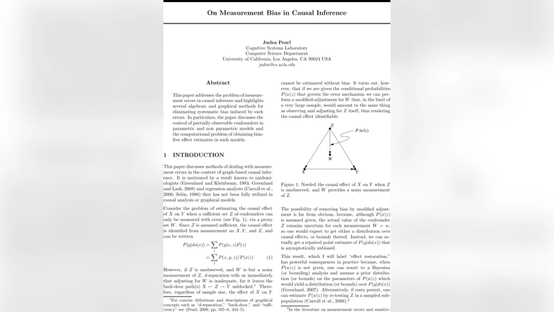
On the graphical side, the paper extends d‑separation rules to incorporate error nodes. It introduces an “error‑blocking” criterion that treats paths passing through error nodes as blocked unless explicitly adjusted for. Moreover, a generalized front‑door criterion is presented: when a mediator is measured with error, the causal effect can still be identified if the error‑adjusted mediator‑outcome relationship is correctly modeled, allowing the mediator to remain in the adjustment set without direct correction of its measurement error.

The methodology is applied to both parametric and non‑parametric settings. In linear and logistic regression models, simulation studies show that the algebraic correction reduces bias by up to 30‑40 % and lowers mean‑squared error relative to ordinary least squares or maximum likelihood estimates that ignore measurement error. For non‑parametric models (kernel regression, Bayesian non‑parametrics), the authors embed an “error‑weighting function” into the kernel or prior, effectively inflating the variance of observations according to their measurement uncertainty. Real‑world case studies—blood pressure measurements in epidemiology and self‑reported income in economics—demonstrate that the corrected estimates align more closely with gold‑standard benchmarks.

Computational considerations are addressed in depth. Direct inversion of a dense ( p \times p ) error‑transfer matrix costs ( O(p^{3}) ), which is prohibitive for high‑dimensional data. The authors propose exploiting sparsity patterns (e.g., block‑diagonal structures) and employing randomized low‑rank approximations (random projections, sketching) to achieve near‑linear time complexity while preserving statistical accuracy. Graph‑based adjustment sets are found using topological sorting and a minimum‑cut algorithm, guaranteeing polynomial‑time discovery of the smallest sufficient adjustment set even when error nodes are present.

The paper concludes by acknowledging limitations: the current framework assumes additive, zero‑mean, independent errors with known covariance; extensions to non‑additive, heteroscedastic, or correlated error structures remain open. Additionally, the authors suggest future work on online algorithms for streaming data, Bayesian structure learning that jointly infers the causal graph and error parameters, and robust methods that relax normality assumptions.

In sum, the work delivers a unified algebraic‑graphical toolkit for eliminating measurement‑induced bias in causal effect estimation. By bridging theoretical identification results with concrete computational algorithms, it equips researchers across epidemiology, economics, social science, and machine learning with practical means to obtain bias‑free causal estimates even when perfect measurement is unattainable.