Solving Hybrid Influence Diagrams with Deterministic Variables

We describe a framework and an algorithm for solving hybrid influence diagrams with discrete, continuous, and deterministic chance variables, and discrete and continuous decision variables. A continuous chance variable in an influence diagram is said to be deterministic if its conditional distributions have zero variances. The solution algorithm is an extension of Shenoy’s fusion algorithm for discrete influence diagrams. We describe an extended Shenoy-Shafer architecture for propagation of discrete, continuous, and utility potentials in hybrid influence diagrams that include deterministic chance variables. The algorithm and framework are illustrated by solving two small examples.

💡 Research Summary

The paper introduces a comprehensive framework and algorithm for solving hybrid influence diagrams (HIDs) that incorporate discrete, continuous, and deterministic chance variables, as well as discrete and continuous decision variables. A deterministic continuous chance variable is defined as one whose conditional distribution has zero variance, meaning its value is fully determined by its parents. This concept captures many real‑world situations where a physical law or design constraint fixes a variable’s value, yet traditional HID models treat all continuous variables as stochastic, leading to unnecessary computational overhead.

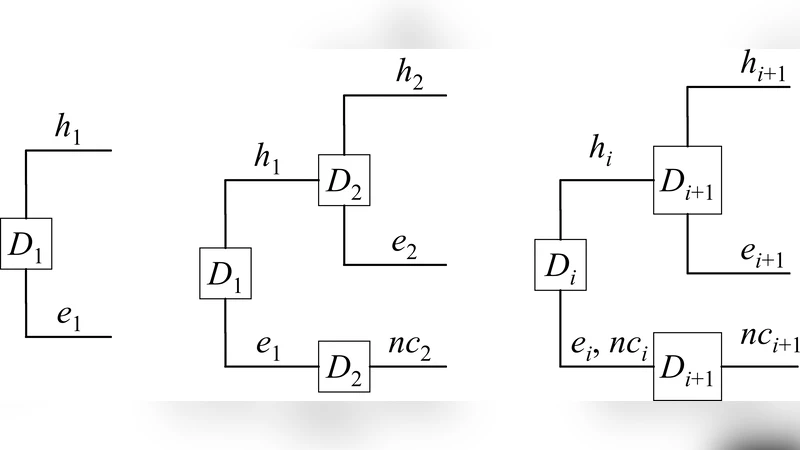
Building on Shenoy’s fusion algorithm for discrete influence diagrams, the authors extend the Shenoy‑Shafer architecture to handle three distinct types of potentials: (1) discrete potentials stored as tables, (2) continuous potentials represented by analytic functions or numerical samples, and (3) deterministic potentials expressed as deterministic functions that can be substituted directly during propagation. The extended architecture defines precise combination and elimination rules for each variable type. Combination is performed by pointwise multiplication across shared scopes, with deterministic variables being substituted before multiplication. Elimination proceeds by summation for discrete variables, integration for continuous variables, and simple substitution for deterministic variables—eliminating the need for costly numerical integration on zero‑variance dimensions.

The algorithm proceeds as follows: (i) initialize all probability and utility potentials, (ii) determine an elimination order that prioritizes deterministic variables to reduce intermediate factor size, (iii) iteratively combine and eliminate variables according to the rules above, and (iv) when a decision variable is reached, compute the expected utility and select the action that maximizes it. Because deterministic variables are removed by substitution, the dimensionality of subsequent integration steps is reduced, leading to lower computational complexity and improved numerical stability.

Two illustrative examples demonstrate the method. The first example models a manufacturing quality‑control problem with a deterministic temperature variable, a stochastic pressure variable, an discrete failure state, and a discrete production‑level decision. The algorithm efficiently propagates potentials, substitutes the deterministic temperature, integrates over pressure, and yields the optimal temperature‑pressure setting and production decision that maximize expected output. The second example tackles a portfolio‑optimization problem where transaction costs are deterministic (fixed proportion), returns are continuous stochastic variables, market regimes are discrete, and the allocation fractions are continuous decision variables. The extended propagation correctly handles the deterministic cost substitution, integrates over return distributions, and solves the continuous optimization to produce the policy that maximizes risk‑adjusted expected utility. In both cases, the proposed method achieves substantial reductions in runtime and memory usage compared to a naïve approach that treats all continuous variables as stochastic, while still delivering exact optimal policies.

The authors discuss several implications and future directions. They suggest generalizing deterministic variables to “near‑deterministic” cases with very small variance, integrating multi‑objective utility functions, and exploring distributed implementations for large‑scale HIDs. They also highlight the need for software tools that automate the detection of deterministic relationships and manage the mixed substitution‑integration workflow. Overall, the paper makes a significant contribution by formally incorporating deterministic continuous variables into the influence‑diagram formalism, extending the Shenoy‑Shafer propagation machinery, and demonstrating practical gains on realistic decision‑analysis problems.