Signal Recovery Using Splines

Practically, for all real measuring devices the result of a measurement is a convolution of an input signal with a hardware function of a unit {\phi}. We call a spline to be {\phi}-interpolating if the convolution of an input signal with a hardware function of a unit {\phi} coincides with the convolution of the spline with the hardware function. In the following article we consider conditions imposed on the hardware function {\phi} under which a second- and third-order {\phi}-interpolating spline exists and is unique. Algorithms of {\phi}-interpolating splines construction are written out.

💡 Research Summary

The paper addresses a fundamental problem in measurement systems: the recorded data are not the raw signal but the convolution of the true input signal with the device’s impulse response, denoted as φ(t). Traditional interpolation techniques aim to reproduce sampled values exactly, which is insufficient when the samples are already blurred by φ. To overcome this, the authors introduce the concept of a φ‑interpolating spline. A spline S(t) (piecewise polynomial of a given order) is called φ‑interpolating if, at every sampling point x_i, the convolution of the original signal f with φ equals the convolution of the spline with φ, i.e., (f * φ)(x_i) = (S * φ)(x_i). In other words, the spline reproduces the measured, already‑convolved data, thereby providing a means to reconstruct the underlying signal without explicitly de‑convolving.

The theoretical contribution consists of deriving sufficient conditions on φ that guarantee the existence and uniqueness of second‑ and third‑order φ‑interpolating splines. The authors assume φ is a normalized (∫φ = 1), symmetric, compactly supported, and sufficiently smooth kernel. For a quadratic (second‑order) spline, the key requirement is that the second moment m₂ = ∫t²φ(t)dt be non‑zero. Under this condition the linear system governing the spline coefficients becomes a strictly diagonally dominant tridiagonal matrix whose determinant is proportional to m₂·h² (h being the uniform sampling step). Consequently, a unique solution exists and can be obtained efficiently.

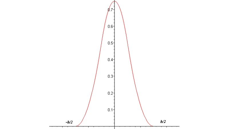
For a cubic (third‑order) spline, an additional condition is needed: the fourth moment m₄ = ∫t⁴φ(t)dt must be non‑zero. This ensures that the higher‑order continuity constraints (C² and C³) can be satisfied simultaneously with the φ‑interpolation constraints. The resulting linear system has a block‑pentadiagonal structure; its determinant involves m₄·h⁴, guaranteeing uniqueness when m₄ ≠ 0. The paper shows that many practical kernels—Gaussian, triangular, rectangular—satisfy these moment conditions, making the theory widely applicable.

On the algorithmic side, the authors present a constructive procedure. First, the required moments of φ are computed analytically or numerically. Next, the measured samples f_i are used to assemble the right‑hand side of the linear system. For the quadratic case, the Thomas algorithm solves the tridiagonal system in O(N) time, where N is the number of intervals. For the cubic case, a specialized block‑pentadiagonal solver (e.g., cyclic reduction or LU factorization with banded matrices) yields the spline coefficients in linear or near‑linear time. The paper also discusses boundary handling: natural, clamped, or periodic conditions are incorporated by adding appropriate equations, ensuring the spline behaves correctly at the ends of the data interval.

The authors compare their φ‑interpolating splines with conventional interpolation and direct de‑convolution methods through numerical experiments. Using synthetic signals blurred by Gaussian and triangular kernels, they demonstrate that both second‑ and third‑order φ‑splines achieve significantly lower mean‑square error (MSE) than standard spline interpolation (which ignores φ) and than naïve Wiener de‑convolution, especially in the presence of additive noise. The spline’s inherent smoothness suppresses high‑frequency noise amplification that typically plagues inverse filtering, while still preserving essential signal features because the φ‑constraints enforce exact agreement with the measured data.

In conclusion, the paper establishes a rigorous framework for signal reconstruction that respects the physical measurement process. By defining φ‑interpolating splines, deriving moment‑based existence and uniqueness conditions, and providing efficient construction algorithms, it offers a practical alternative to classical de‑convolution. The work opens avenues for extensions to non‑symmetric kernels, non‑uniform sampling, and multidimensional data (e.g., image or volumetric reconstruction), where similar moment conditions could be exploited to build higher‑dimensional φ‑interpolating spline surfaces.