A Dirty Model for Multiple Sparse Regression

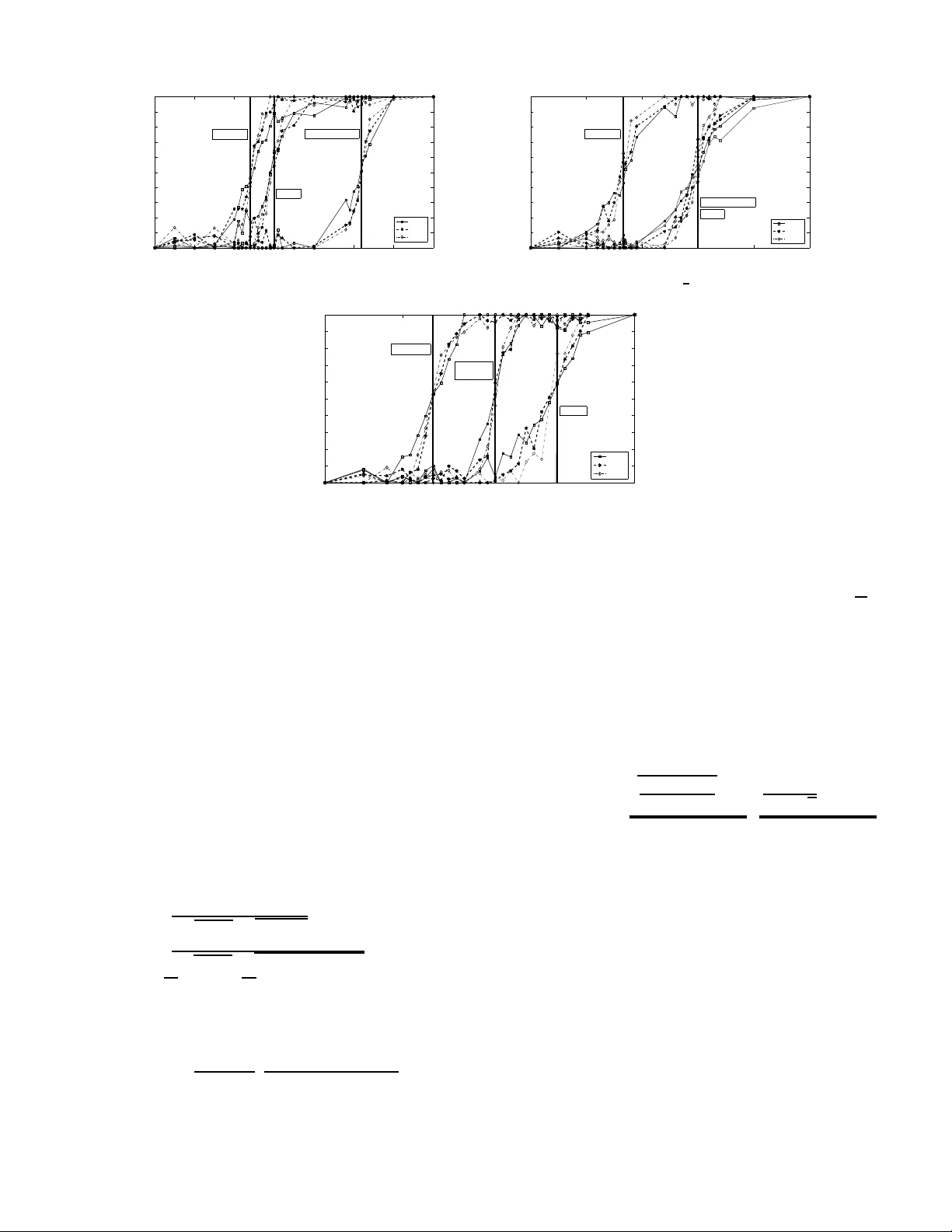
1 A Dirty Model for Mult iple Sparse Re gression Ali Jalali, Pradeep Ra vikumar, and Sujay Sanghavi, Member Abstract —Sparse linear re gression – ﬁnding an unknown vector from linear measurem ents – is now known to be possible with fewer samples than variables, via methods like th e LASSO. W e consider th e multip le sparse linear regression problem, where sev eral related vectors – with p artially shared support sets – hav e to b e recov ered. A natural question in this setting is wh ether one can u se the sharing to furth er decrease the overall nu mber of samples required. A lin e of recent resea rch has studied the use of ℓ 1 /ℓ q norm block-regularizations with q > 1 f or such p roblems; howev er these could actually perfo rm worse in sample complexity – vis a vis solving each problem separately ignoring sh aring – dependin g on the le vel of sharing . W e present a new method for mu ltiple sparse l inear regr ession that can lever age support and parameter over lap when it exists, but not pay a penalty when it does not. a very simple idea: we decompose the parameters into two components and regularize these diff erently . W e show b oth theoretically and empirically , our method strictly and noticeably outperfo rms both ℓ 1 or ℓ 1 /ℓ q methods, over the en tire range of possible o ver laps (except at boundary cases, where we match the b est method). W e also prov ide theoretical guarantees that the method perfo rms well under high-dimensional scaling. Index T erms —Multi-task Learning, High-dimensional S tatis- tics, Multiple Regression. I . I N T R O D U C T I O N : M O T I V AT I O N A N D S E T U P High-dimen sional scaling. In ﬁelds across science and eng i- neering, we are increasingly faced with problem s where the number o f variables or features p is larger than the numb er of observations n . Under such h igh-dim ensional scaling , for any hope of statis tically consistent estimation, it becomes vital to lev erage any potential structure in the pr oblem such as sparsity (e.g. in co mpressed sensing [ 3] an d LASSO [17]), low-rank structure [1 6, 12], o r spar se graphic al model structure [15]. It is in such high-d imensional contexts in p articular tha t multi- task learning [4] cou ld be most usefu l. Her e, multiple tasks share some common stru cture such as spar sity , and estimating these tasks jointly b y leveraging this common structure could be more s tatistically ef ﬁcient. Block-sparse Mu ltiple Regr ession. A common multiple task learning settin g, and which is the focu s of this paper, is tha t o f multiple re gression, where we have r > 1 response v ar iables, and a common set of p featur es or cov ariates. The r tasks could share certain aspects of th eir under lying d istributions, such as common variance, but the setting we focus on in this paper is wh ere the r esponse variables have simultaneously sparse structure: th e index set o f r elev an t features for each task is sparse; and th ere is a large overlap of these relev an t features across the different regression problem s. Such “simultan eous sparsity” arises in a variety of contexts [18]; indee d, mo st The authors are with the Departments of Electrical and Computer Engineer - ing (Jalali and Sanghavi ) and Computer Science (Ravikumar), The Uni ver sity of T exas at Austin, Austin, TX 78712 USA email: (alij@mail.ut exa s.edu; pradeep r@cs.ute xas.edu; sanghav i@mail.ut exa s.edu) applications of sparse signal recovery in con texts ran ging from g raphical mo del lea rning, kern el learn ing, an d fu nction estimation ha ve natura l exten sions to the simultaneous-spar se setting [15, 2 , 14]. It is u seful to represent the multiple regression par ameters via a matrix, where each colu mn corresp onds to a task , and each row to a feature. Having simultaneou s spar se struc ture then cor respond s to the matrix b eing largely “block -sparse” – where each row is e ither a ll ze ro o r m ostly no n-zero , an d the number o f non -zero rows is small. A lot of recen t research in this setting has fo cused on ℓ 1 /ℓ q norm regularizations, f or q > 1 , that encoura ge the parameter matrix to hav e such block- sparse stru cture. P ar ticular examples include results using the ℓ 1 /ℓ ∞ norm [19, 5, 11], and the ℓ 1 /ℓ 2 norm [10, 13]. Our Mo del. Block-regu larization is “h eavy-handed” in two ways. By strictly encouraging shared -sparsity , it ass umes that all relev an t featu res are shared , an d h ence suffers under settings, arguably more realistic, where each task depends o n features speciﬁc to its elf in addition to th e ones that ar e com- mon. The second concern with such block-sp arse regu larizers is th at the ℓ 1 /ℓ q norms ca n b e shown to en courag e the en tries in the non-spar se rows taking nearly identical v alues . Thus we are far aw ay f rom the orig inal goal of m ultitask learn ing: not only do the set of relev an t features have to be e xactly the same, but th eir values have to a s well. Ind eed r ecent re search into such regularized meth ods [11, 13] cau tion again st the use of block-r egularization in regimes where the suppo rts and values of the par ameters for each task can vary widely . Since the true parameter values are unknown, t hat would be a worriso me cav eat. W e thus ask the question: can we lear n m ultiple r egression models by leveraging wha tev er overlap o f featur es there exist, and without requirin g the par ameter values to b e near iden- tical? Indee d this is an in stance of a more gen eral que stion on whether we can estima te statistical mo dels wh ere the data may n ot fall clea nly into any on e structur al b racket (sparse, block-spa rse and so on ). W ith th e explosion of complex and dirty h igh-dim ensional data in mo dern settings, it is vital to in vestigate estimation of correspon ding dirty mod els, which might require n ew app roaches to biased high -dimen sional estimation. In this p aper we take a ﬁrst step, fo cusing on su ch dirty mod els for a speciﬁc p roblem: simultaneou sly sparse multiple regression. Our appro ach uses a simple idea: wh ile any o ne structure might not captur e the data, a superposition of structura l class es might. Our method thus search es for a parameter matrix that can be decomp osed into a row-sparse matrix (corre sponding to the overlapping o r share d featu res) and an elementwise sparse matrix (corresp onding to the non -shared featur es). As we show both theoretically an d em pirically , with this simple ﬁx we are able to leverage any extent of sha red featu res, while 2 allowing disparities in support and values of the parameter s, s o that we are always better than both th e Lasso or block -sparse regularizers (at times remarkab ly so). The r est of the paper is organized as follows: In Sec 2. basic deﬁnitions and setup of the prob lem are presented . Ma in results o f the pa per is discussed in sec 3. Exp erimental results and simulations are dem onstrated in Sec 4. Notatio n: For any ma trix M , we denote its j th row as m j , and its k -th column as m ( k ) . The set of all non- zero rows (i.e. all rows with at least on e n on-zero element) is denoted by RowSupp ( M ) and its su pport by Supp ( M ) . Also, for any matrix M , let k M k 1 , 1 := P j,k | m ( k ) j | , i.e. the sums of absolute v alu es o f the elemen ts, and k M k 1 , ∞ := P j k m j k ∞ where, k m j k ∞ := max k | m ( k ) j | . I I . P RO B L E M S E T - U P A N D O U R M E T H O D Multiple r e g r ession . W e consider the following s tandard mul- tiple linear regression model: y ( k ) = X ( k ) ¯ θ ( k ) + w ( k ) , k = 1 , . . . , r , where, y ( k ) ∈ R n is the response for the k -th task, r egressed on the design matrix X ( k ) ∈ R n × p (possibly different across tasks), while w ( k ) ∈ R n is the noise vector . W e assume each w ( k ) is d rawn indepe ndently fro m N (0 , σ 2 ) . The total nu mber of tasks or target variables is r , the number o f features is p , while the n umber o f samples we have f or each task is n . For notational convenience, we collate these qua ntities into matrices Y ∈ R n × r for the respon ses, ¯ Θ ∈ R p × r for the regression p arameters and W ∈ R n × r for the noise. Our Model. In this paper we are inter ested in estimating the true par ameter ¯ Θ from d ata { y ( k ) , X ( k ) } by leveraging any (un known) extent o f simultaneou s-sparsity . In particular, certain ro ws of ¯ Θ w ould ha ve many non-ze ro entries, correspo nding to features share d by several tasks (“shared” rows), while certain rows would be elementwise s parse, correspo nding to tho se f eatures wh ich are relevant f or som e tasks but not all (“non-shared rows”), while certain rows would hav e all ze ro entries, cor respond ing to tho se features that are not relev ant to any task. W e are in terested in estimators b Θ that autom atically adapt to d ifferent le vels of sharedness, and y et enjoy th e follo wing g uarantees: Support recovery: W e say an estimator b Θ successfully recovers the tru e sign ed sup port if sign ( Supp ( b Θ)) = sign ( Supp ( ¯ Θ)) . W e are in terested in deriving su fﬁcient co nditions u nder which the estimator succeed. W e note that this is st ronger than me rely recovering the row-support of ¯ Θ , which is union of its supp orts fo r the different tasks. In pa rticular, de noting U k for the sup port o f the k -th column of ¯ Θ , and U = S k U k . Error bounds: W e are also interested in providing bo unds on the elementwise ℓ ∞ norm error o f the e stimator b Θ , k b Θ − ¯ Θ k ∞ = max j =1 ,...,p max k =1 ,...,r    b Θ ( k ) j − ¯ Θ ( k ) j    . A. Our Method Our metho d models the un known para meter Θ as a su- perposition of a block- sparse matrix B (cor respond ing to the features shared across many tasks) and a sparse m atrix S (cor respond ing to the features shar ed acro ss few tasks). W e estimate th e sum of two par ameter m atrices B and S with different regular izations fo r each : encou raging block- structured row-sparsity in B and elementwise sparsity in S . The c orrespon ding simple mod els would either just use block- sparse regularizations [ 11, 13] or ju st elementwise sparsity regularizations [17, 21], so that eithe r meth od would per- form be tter in certain suited regimes. Interestin gly , as we will see in the ma in results, by explicitly allowing to ha ve both block-sp arse and elemen twise spar se co mpon ent (see Algorithm II-A), we are able to outperform both classes of these “clean models”, for all regimes ¯ Θ . I I I . M A I N R E S U LT S A N D T H E I R C O N S E Q U E N C E S W e now provide precise statements of our main results. A number of recen t results have shown that the Lasso [1 7, 21] and ℓ 1 /ℓ ∞ block-r egularization [ 11] methods succe ed in model selection, i.e., re covering signed supp orts with co n- trolled err or bound s under high-d imensional scaling regimes. Our ﬁrst two theorem s extend these resu lts to ou r mode l setting. In Theorem 1, we con sider th e case of determin istic design matrices X ( k ) , and provide sufﬁcient conditions guar - anteeing sign ed suppo rt recovery , and elementwise ℓ ∞ norm error b ounds. In Theorem 2, we specialize this the orem to the case where the ro ws of the design matr ices are ran dom from a gen eral zero mean Gaussian distrib ution: this allows us to provide scaling on the number of observ ations re quired in order to guara ntee sign ed support recovery and bou nded elementwise ℓ ∞ norm error . Our th ird r esult is th e most interesting in th at it explicitly quantiﬁes the performan ce gains of our method vis-a-vis Lasso and the ℓ 1 /ℓ ∞ block-r egularization method. Since this entailed ﬁnding th e pr ecise con stants und erlying earlier theorems, and a correspo nding ly more delicate an alysis, we f ollow Ne g ahban and W ain wright [11] and fo cus on the case where there are two-tasks (i.e. r = 2 ), and whe re we hav e standard Gaussian design matrices as in Theorem 2. Further, while each of two tasks depends on s features, only a fraction α of these are common . It is then interesting to see how the behaviors o f the different regularization meth ods vary with the extent of overlap α . Comparisons. Negah ban and W ainwrigh t [1 1] show tha t there is ac tually a “phase tr ansition” in the scaling of the pro bability of successful signed support-recovery with the nu mber of observations. De note a particular rescaling of the sample- size θ Lasso ( n, p , α ) = n s log( p − s ) . Then a s W ainwrigh t [21] show , when the rescaled number of samp les scale s as θ Lasso > 2 + δ for a ny δ > 0 , L asso succeed s in re covering the sign ed support o f all columns with pro bability converging to one. But wh en the sample size scales as θ Lasso < 2 − δ for a ny δ > 0 , Lasso fails with probab ility conver ging to on e. For th e ℓ 1 /ℓ ∞ -regularized m ultiple linear regression, deﬁne a similar rescaled s ample s ize θ 1 , ∞ ( n, p , α ) = n s log( p − (2 − α ) s ) . Then as 3 Algorithm 1 Complex B lock Sparse Solve the f ollo wing con vex optimization p roblem: ( b S , b B ) ∈ arg min S,B 1 2 n r X k =1    y ( k ) − X ( k )  s ( k ) + b ( k )     2 2 + λ s k S k 1 , 1 + λ b k B k 1 , ∞ . (1) Then output b Θ = b B + b S . Negahban and W ainwrigh t [11] s how there is again a transition in prob ability o f success from near zer o to near one, at the rescaled sample size of θ 1 , ∞ = (4 − 3 α ) . Thus, for α < 2 / 3 (“less sharin g”) Lasso would pe rform better since its transition is at a smaller sample size, while for α > 2 / 3 (“mo re sharing”) the ℓ 1 /ℓ ∞ regularized m ethod w ould perform b etter . As we show in o ur th ird th eorem, th e ph ase transition fo r our m ethod occur s at th e rescaled sample size of θ 1 , ∞ = (2 − α ) , which is strictly before either the Lasso or the ℓ 1 /ℓ ∞ regularized method except for the bound ary cases: α = 0 , i.e. th e case o f no sharing, where we match Lasso, and for α = 1 , i.e. full sharin g, where we match ℓ 1 /ℓ ∞ . Everywhere else, we strictly outperform both methods. Figure III sho w s the empirical perform ance of each of the three metho ds; as can be seen, they agree very well with the th eoretical analysis. (Further details in th e e xperiments Section I V). A. Sufﬁcient Conditions for Deterministic Designs W e ﬁrst consider the case wher e the design matr ices X ( k ) for k = 1 , · · · , r are deterministic, and start by specif ying the assumption s we impose on the m odel. W e n ote that similar sufﬁcient cond itions for th e d eterministic X ( k ) ’ s case we re imposed in p apers a nalyzing Lasso [21] and block-r egularization m ethods [11, 13]. A0 Column Normalization: k X ( k ) j k 2 ≤ √ 2 n for a ll j = 1 , . . . , p and k = 1 , . . . , r . A1 Incoherence Con dition: γ b := 1 − max j ∈U c r X k =1      X ( k ) j , X ( k ) U k D X ( k ) U k , X ( k ) U k E − 1      1 > 0 , where, U k denotes the su pport of th e k -th co lumn of ¯ Θ , and U = S k U k denotes th e union of the suppo rts of all tasks. W e will also ﬁnd it useful to deﬁne γ s := 1 − max 1 ≤ k ≤ r max j ∈U c k     D X ( k ) j , X ( k ) U k E D X ( k ) U k , X ( k ) U k E − 1     1 . Note that by the incoh erence co ndition A 1 , we ha ve γ s > 0 . A2 Minimum Curvatur e Condition: C min := min 1 ≤ k ≤ r λ min  1 n D X ( k ) U k , X ( k ) U k E  > 0 . Also, de ﬁne D max := max 1 ≤ k ≤ r       1 n D X ( k ) U k , X ( k ) U k E  − 1      ∞ , 1 . As a consequen ce of A2 , we ha ve that D max is ﬁnite. A3 Regularizers: W e requ ire the r egularization param eters satisfy A3-1 λ s > 2(2 − γ s ) σ √ log( pr ) γ s √ n . A3-2 λ b > 2(2 − γ b ) σ √ log( pr ) γ b √ n . A3-3 1 ≤ λ b λ s ≤ r and λ b λ s is not an integer (see Lemma 11 and 12 for the reason). Theorem 1. Suppo se A0-A3 hold, and that we obtain estimate b Θ fr om our algorithm. Then, with pr o bability at least 1 − c 1 exp( − c 2 n ) , we ar e gu aranteed that the conve x pr ogram (1) has a u nique optimum and (a) The estimate b Θ has n o false inc lusions, and ha s bound ed ℓ ∞ norm err o r: Supp ( b Θ) ⊆ Supp ( ¯ Θ) , and k b Θ − ¯ Θ k ∞ , ∞ ≤ r 4 σ 2 log ( pr ) n C min + λ s D max | {z } b min . (2) (b) The estimate b Θ has no false exclusions, i.e., sign ( Supp ( b Θ)) = sign  Supp ( ¯ Θ)  pr ovided that min ( j,k ) ∈ Supp ( ¯ Θ)    ¯ θ ( k ) j    > b min for b min deﬁned in p art (a). The positive co nstants c 1 , c 2 depend only o n γ s , γ b , λ s , λ b and σ , but are otherwise indep endent of n, p, r , the pr ob lem dimensions of in ter est. Remark: Con dition (a) guaran tees that the estimate will have no false inclusions ; i.e. all included features will be relev an t. If in ad dition, we require that it have no false exclusions and that recover th e sup port exactly , we need to impose the assumption in (b) tha t th e non-ze ro elements are large eno ugh to be detectab le above the n oise. B. General Gaussian Designs Often the design matrices consist of samples from a Gaussian ensemble (e.g. in Gaussian graphical model structure learnin g). Supp ose th at for each task k = 1 , . . . , r the design matrix X ( k ) ∈ R n × p is such th at each row X ( k ) i ∈ R p is a zero-m ean Gau ssian random vector with covariance ma trix Σ ( k ) ∈ R p × p , and is in depend ent of every other row . Let Σ ( k ) V , U ∈ R |V |×|U | be the sub matrix of Σ ( k ) with correspon ding rows to V and column s to U . W e require these cov arian ce ma trices to satisfy the following cond itions: C1 Incoher ence Con dition: γ b := 1 − ma x j ∈U c r X k =1     Σ ( k ) j, U k ,  Σ ( k ) U k , U k  − 1     1 > 0 4 0.5 1 1.5 1.7 2 2.5 3 3.1 3.5 4 0 0.1 0.2 0.3 0.4 0.5 0.6 0.7 0.8 0.9 1 Control Parameter θ Probability of Success p=128 p=256 p=512 Dirty Model LASSO L1/Linf Reguralizer (a) α = 0 . 3 0.5 1 1.333 1.5 2 2.5 3 0 0.1 0.2 0.3 0.4 0.5 0.6 0.7 0.8 0.9 1 Control Parameter θ Probability of Success p=128 p=256 p=512 Dirty Model L1/Linf Reguralizer LASSO (b) α = 2 3 0.5 1 1.2 1.5 1.6 2 2.5 0 0.1 0.2 0.3 0.4 0.5 0.6 0.7 0.8 0.9 1 Control Parameter θ Probability of Success p=128 p=256 p=512 Dirty Model L1/Linf Reguralizer LASSO (c) α = 0 . 8 Fig. 1. P robability of success in recovering the true signed support using dirty mod el, Lasso and ℓ 1 /ℓ ∞ regularizer . F or a 2 -task pro blem, the probability of success for different v alues of feature-ov erlap fraction α is plotted. As we can see in the regimes that Lasso is better than, as good as and worse t han ℓ 1 /ℓ ∞ regularizer ((a), (b) and (c) respectiv ely), the dirty model outperforms both of the methods, i. e., it requires less numb er of obse rv ations for successful recovery o f the true signed support comp ared to Lasso and ℓ 1 /ℓ ∞ regularizer . Here s = ⌊ p 10 ⌋ alway s. . C2 Minimum Curvatur e Condition: C min := min 1 ≤ k ≤ r λ min  Σ ( k ) U k , U k  > 0 and let D max :=      Σ ( k ) U k , U k  − 1     ∞ , 1 . These con ditions are analo gues of the conditio ns for deterministic d esigns; they ar e now impo sed on the covariance matrix o f the (r andom ly ge nerated) rows o f the design matrix. C3 Regularizers: Deﬁning s := max k |U k | , we require th e regularization p arameters satisfy C3-1 λ s ≥ ( 4 σ 2 C min log( pr ) ) 1 / 2 γ s √ nC min − √ 2 s log( pr ) . C3-2 λ b ≥ ( 4 σ 2 C min r ( r log(2)+log ( p )) ) 1 / 2 γ b √ nC min − √ 2 sr ( r log(2)+l og( p )) . C3-3 1 ≤ λ b λ s ≤ r and λ b λ s is not an integer . Theorem 2. Suppose assumptio ns C1-C3 hold, a nd tha t the number of sa mples scale as n > max 2 s log( p r ) C min γ 2 s , 2 sr  r log ( 2) + log ( p )  C min γ 2 b ! . Suppo se we obtain estimate b Θ fr om our a lgorithm. Th en, with pr oba bility a t least 1 − c 1 exp ( − c 2 ( r lo g(2) + log ( p ))) − c 3 exp( − c 4 log( r s )) → 1 for some positive numbers c 1 − c 4 , we ar e guaranteed that the algorith m estimate b Θ is un ique an d satisﬁes the following condition s: (a) The estimate b Θ has n o false inc lusions, and ha s bound ed ℓ ∞ norm err o r so that Supp ( b Θ) ⊆ Supp ( ¯ Θ) , and k b Θ − ¯ Θ k ∞ , ∞ ≤ r 50 σ 2 log( r s ) nC min + λ s  4 s C min √ n + D max  | {z } g min . (3) (b) The estimate b Θ has no false exclusions, i.e., sign ( Supp ( b Θ)) = sign  Supp ( ¯ Θ)  pr ovided that min ( j,k ) ∈ Supp ( ¯ Θ)    ¯ θ ( k ) j    > g min for g min deﬁned in part (a ). C. Quantifying the gain for 2 -T ask Gaussian Designs This is one of th e m ost importan t results of th is pap er . Here, we perform a mo re delicate a nd ﬁner analysis to establish precise quantitative gains of o ur method. W e focus on the special case where r = 2 and the desig n matrix has rows generated from the s tandard Gaussian distribution N (0 , I n × n ) . As we will see both analytically and experimentally , o ur method strictly outperfor ms both Lasso and ℓ 1 /ℓ ∞ -block- regularization over for all cases, except at the extreme end- points of no s uppor t sharing ( where it matches that o f Lasso) and full sup port sharing (wh ere it ma tches that of ℓ 1 /ℓ ∞ ). W e now pre sent our analytical results; the empirical com parisons 5 are p resented next in Section IV. The r esults will be in terms of a particular rescaling of the sample size n as θ ( n, p, s, α ) := n (2 − α ) s log ( p − (2 − α ) s ) . W e also require that the regularizer s satisfy F1 λ s >  4 σ 2 (1 − p s/n )(log( r ) + log( p − (2 − α ) s ))  1 / 2 √ n − √ s − ((2 − α ) s (log ( r ) + log ( p − (2 − α ) s ))) 1 / 2 . F2 λ b >  4 σ 2 (1 − p s/n ) r ( r log (2) + log ( p − (2 − α ) s ))  1 / 2 √ n − √ s − ((1 − α/ 2) sr ( r log(2) + log( p − (2 − α ) s ))) 1 / 2 . F3 λ b λ s = √ 2 . Theorem 3. Consider a 2 -task re gr ession pr oblem ( n, p, s, α ) , wher e the design matrix h as r ows generated fr om the standard Gaussian distrib ution N (0 , I n × n ) . Suppose max j ∈ B ∗         Θ ∗ (1) j    −    Θ ∗ (2) j         ≤ cλ s , wher e, B ∗ is the sub matrix of Θ ∗ with r ows wher e b oth entries ar e no n-zer o and c is a constant speciﬁed in Lemma 7 . Then the estimate b Θ of the p r oblem (1) satisﬁes th e following: ( Success ) Supp ose the r e g ularization coefﬁcients satisfy F1 − F3 . Further , assume th at the number of samples scales as θ ( n, p, s, α ) > 1 . Then, with pr oba bility at least 1 − c 1 exp( − c 2 n ) for some positive numb ers c 1 and c 2 , we ar e guaranteed tha t b Θ satisﬁes the suppo rt-r ecovery and ℓ ∞ err or bound conditions (a-b) in Theorem 2. ( Failure ) If θ ( n, p, s, α ) < 1 ther e is no solutio n ( ˆ B , ˆ S ) for any choice s of λ s and λ b such that sign  Supp ( b Θ)  = sign  Supp ( ¯ Θ)  . Remark: The ass umption on the gap       Θ ∗ (1) j    −    Θ ∗ (2) j       ≤ cλ s reﬂects the fact that we require that most v alues of Θ ∗ to be balanced o n both tasks on the shared suppo rt. As we show in a mo re general theo rem (Theor em 4) in Section VI-C, ev en in the ca se where the gap is lar ge, the depen dence of the sample scaling on th e gap is qu ite weak. I V . S I M U L AT I O N R E S U LT S In this section, we provide som e simu lation results. First, using our synthetic data set, we inv estigate the consequences of Theo rem 3 wh en we ha ve r = 2 tasks to learn. As we see, the emp irical resu lt veriﬁes our theor etical gu arantees. Next, we apply o ur method regression to a r eal datasets: a hand - written d igit classiﬁcation dataset with r = 10 ta sks (equ al to the num ber of d igits 0 − 9 ). For this dataset, we show th at our method outperf orms both LASSO an d ℓ 1 /ℓ ∞ practically . For each metho d, the parameter s are chosen via cro ss-validation; see supplemental material fo r more d etails. A. Synthetic Data Simulation Consider a r = 2 -task r egression pr oblem of the fo rm ( n, p , s, α ) as d iscussed in Theorem 3. For a ﬁxed set of parameters ( n, s, p, α ) , we generate 100 instan ces of th e problem . Th en, we solv e the sam e problem using our model, ℓ 1 /ℓ ∞ regularizer and LASSO by searchin g for penalty regularizer coefﬁcients in depend ently for each on e of these progr ams to ﬁnd the best regularizer b y cr oss validation. After solving th e thr ee p roblems, we co mpare the sign ed supp ort of the solution with the true signed supp ort and decide whe ther or not the pro gram was successful in sign ed su pport recovery . W e describe these process in more details in th is section. Data Generat ion : W e explain how we gen erated the d ata for o ur simu lation h ere. W e p ick thre e different values of p = 1 2 8 , 256 , 5 12 an d let s = ⌊ 0 . 1 p ⌋ . F or d ifferent values of α , we let n = c s log( p − (2 − α ) s ) for different values of c . W e gener ate a rand om sign matrix e Θ ∗ ∈ R p × 2 (each entry is either 0 , 1 o r − 1 ) with co lumn suppo rt size s and row support size (2 − α ) s as r equired by Th eorem 3. Th en, we multiply each row by a real random numb er with magn itude g reater than th e minimu m requ ired f or sign support recovery by T heorem 3. W e genera te two sets of matrices X (1) , X (2) and W and use on e of them for training and the other on e for cross validation (test), sub scripted T r and T s, r espectively . Each en try o f the n oise matrices W Tr , W Ts ∈ R n × 2 is drawn indep enden tly acco rding to N (0 , σ 2 ) where σ = 0 . 1 . Each row of a design matrix X ( k ) Tr , X ( k ) Ts ∈ R n × p is samp led, ind ependen t of any other rows, f rom N (0 , I 2 × 2 ) for all k = 1 , 2 . Having X ( k ) , ¯ T heta and W in h and, we can ca lculate Y Tr , Y Ts ∈ R n × 2 using the model y ( k ) = X ( k ) θ ( k ) + w ( k ) for all k = 1 , 2 for both train and test set of variables. Coordinate Descent Algorithm : Given the gener ated data X ( k ) Tr for k = 1 , 2 a nd Y Tr in the previous section, we want to recover matr ices ˆ B an d ˆ S that satisfy (1 ). W e use the co ordinate d escent algo rithm to numer ically solve the problem ( see Appendix B) . The algo rithm in puts the tuple ( X (1) Tr , X (2) Tr , Y Tr , λ s , λ b , ǫ , B , S ) and outputs a matrix pair ( ˆ B , ˆ S ) . The in puts ( B , S ) are initial g uess and can be set to zero. Howe ver, when we search for optimal penalty regularizer coefﬁcients, we can use the result f or pr evious set of coefﬁcients ( λ b , λ s ) as a go od initial guess for the next coefﬁcients ( λ b + ξ , λ s + ζ ) . The par ameter ǫ cap tures the stoppin g criter ion threshold o f th e algorith m. W e iterate inside the algorithm until the relative upd ate ch ange of the objective function is less than ǫ . Since we do not run the algorithm complete ly ( until ǫ = 0 works), we need to ﬁlter the small magnitude values in the solution ( ˆ B , ˆ S ) and set them to be zero . Choosing penalty regularizer co efﬁcients : Dictated b y optimality cond itions, we have 1 > λ s λ b > 1 2 . Thu s, searching range for one of the coefﬁcients is bo unded and known. W e set λ b = c q r log ( p ) n and sear ch for c ∈ [0 . 01 , 10 0] , where this in terval is partitio ned logar ithmic. For any pair ( λ b , λ s ) we com pute the objec ti ve function of Y Ts and X ( k ) Ts for k = 1 , 2 using the ﬁltered ( ˆ B , ˆ S ) from th e coord inate descen t algorithm . Then across all choices of ( λ b , λ s ) , we pick the one with minim um ob jectiv e f unction on the test data. Finally we let ˆ Θ = Filter ( ˆ B + ˆ S ) for ( ˆ B , ˆ S ) co rrespon ding to the optimal ( λ b , λ s ) . 6 0 0.1 0.2 0.3 0.4 0.5 0.6 0.7 0.8 0.9 1 1 1.5 2 2.5 3 3.5 4 Shared Support Parameter α Phase Transition Threshold p=128 p=256 p=512 LASSO Dirty Model L1/Linf Regularizer Fig. 2. V eriﬁcation of the result of the Theorem 3 on the beha vior of phase transition threshold by changing the parameter α in a 2 -task ( n, p, s, α ) problem for our method, LASSO and ℓ 1 /ℓ ∞ regularizer . The y -axis is n s log ( p − (2 − α ) s ) , where n is the number of samples at which threshold was observ ed. Here s = ⌊ p 10 ⌋ . Our method sho ws a gain in sample complexity over the entire range of sharing α . The pre-constant i n Theorem 3 is also validated. Perf o rmance Analy sis : W e ran the algor ithm for ﬁve different values of the overlap r atio α ∈ { 0 . 3 , 2 3 , 0 . 8 } with three dif ferent numb er of features p ∈ { 128 , 256 , 512 } . For any instance o f the problem ( n, p, s, α ) , if the recovered m atrix ˆ Θ has the same sign supp ort as the true ¯ Θ , then we cou nt it as success, o therwise failure (even if o ne elemen t has different sign, we count it as failure). As T heorem 3 p redicts a nd Fig III sho ws, the right scaling for the nu mber of oservations is n s log( p − (2 − α ) s ) , where all curves stack on the top of each other at 2 − α . Also, the number o f o bservations r equired by o ur model f or true signed support r ecovery is al ways less than bo th LASSO and ℓ 1 /ℓ ∞ regularizer . Fig 1(a) shows the prob ability of su ccess f or th e case α = 0 . 3 (wh en LASSO is better than ℓ 1 /ℓ ∞ regularizer) and that our m odel outp erform s b oth meth ods. When α = 2 3 (see Fig 1(b)), LASSO and ℓ 1 /ℓ ∞ regularizer perf orms the same; but o ur mo del req uire almost 33% less observations for the same per forman ce. As α grows toward 1 , e.g. α = 0 . 8 as shown in Fig 1(c ), ℓ 1 /ℓ ∞ perfor ms better than LASSO. Still, our mo del p erform s better than b oth methods in this case as well. Scaling V eriﬁcatio n : T o verify that the phase tran sition threshold changes lin early with α as pr edicted by Th eorem 3, w e plot the phase transition threshold versus α . For ﬁ ve different values of α ∈ { 0 . 05 , 0 . 3 , 2 3 , 0 . 8 , 0 . 95 } and three different values of p ∈ { 1 28 , 256 , 5 12 } , we ﬁnd th e ph ase transition thresho ld fo r our mo del, LASSO and ℓ 1 /ℓ ∞ regularizer . W e consider th e po int where the prob ability of success in recovery of signed supp ort exceed s 5 0% as the phase transition threshold . W e ﬁnd this po int by interpolation on the closest two points. Fig 2 shows tha t phase tr ansition threshold for ou r mode l is always lower th an the phase transition for LASSO an d ℓ 1 /ℓ ∞ regularizer . B. Handwritten Digits Dataset W e use a han dwritten digit d ataset to illustrate th e perfor mance of our me thod. Accordin g to the d escription of the dataset, this dataset co nsists of features of h andwritten numerals ( 0 - 9 ) extracted from a collectio n o f Dutch utility maps [1]. This data set has been used by a num ber of pap ers [20, 7] as a reliable dataset for han dwritten rec ognition algorithm s. Structure of the Dat aset : In this dataset, th ere ar e 200 instances of handwr itten dig its 0 - 9 (to tally 20 00 digits). Each in stance o f each digit is scanne d to an image of the size 30 × 48 pixels. This imag e is NO T provided by the dataset. Using th e full resolution image of e ach digit, the dataset provides six different classes of features. A total of 649 features are p rovided for each instance of each digit. The info rmation abo ut each class of f eatures is provided in T able I. The combined han dwriting images of the record number 100 is shown in Fig 3 (ten imag es are con catenated together with a spacer between each tw o ). Fitting the dataset to our mo del : Regardless of the nature of the f eatures, we have 6 49 features f or each of 200 instance of eac h digit. W e need to lear n K = 10 d ifferent tasks correspo nding to ten different digits. T o make the associated number s of features comp arable, we shrin k the dynam ic ran ge of each feature to the interval − 1 and 1 . W e d ivide eac h f eature by an approp riate n umber (perhap s larger than the maximum of th at featu re in the dataset) to make sure tha t th e dy namic range of all featu res is a (no t too small) subset o f [ − 1 , 1] . Notice that in this division process, we don ’t care about the minimum and max imum of the trainin g set. W e just divide each feature by a ﬁxed and predetermin ed numb er w e provided as m aximum in T ab le I. For exam ple, we divide the Pixel Shape feature by 6 , Kar hunen -Loeve coefﬁcients by 17 or the last morpho logical feature by 18000 and so o n. W e do not shift the data; we only scale it. Out of 200 sam ples provided f or ea ch digit, we take n ≤ 200 samples for train ing. Let X ( k ) = X ∈ R 10 n × 649 for all 0 ≤ k ≤ 9 be the matr ix whose ﬁrst n rows co rrespon d to the featu res of the d igit 0 , the secon d n rows corre spond to the f eatures of the digit 1 and so on . Con sequently , we set the vector y ( k ) ∈ { 0 , 1 } 10 n to be the vector such that y ( k ) j = 1 if and on ly if th e j th row of the fea ture matrix X correspo nds to the digit k . This setup is called binary classiﬁcation s etup. W e want to ﬁnd a blo ck-sparse matrix ˆ B ∈ R 649 × 10 and a sparse matrix ˆ S ∈ R 649 × 10 , so tha t f or a gi ven fe ature vector x ∈ R 649 extracted from the image of a handwr itten digit 0 ≤ k ∗ ≤ 9 , we ideally hav e k ∗ = arg max 0 ≤ k ≤ 9 x  ˆ B + ˆ S  . T o ﬁnd such m atrices ˆ B an d ˆ S , we solve (1). W e tune the parameter s λ b and λ s in ord er to g et the best result by cross validation. Sinc e we have 10 tasks, we search for λ s λ b ∈  1 10 , 1  and let λ b = c q 2 log (649) n ≈ 5 c √ n , where, empirically c ∈ [0 . 01 , 10 ] is a constant to b e searched. Perf o rmance Analysis : T able II sho ws the results of o ur analysis for different sizes o f the training set as n 200 . W e 7 Fea ture Size T ype Dynamic Range 1 Pixe l Shape ( 15 × 16 ) 240 Int ege r 0-6 2 2D Fourier Transform Coef ﬁ cient s 74 Real 0-1 3 Karhunen-Loe ve Transform Coeﬁcient s 64 Real -17:17 4 Proﬁle Correlation 216 Inte ger 0-1400 5 Zernike Moments 46 Real 0-800 3 Inte ger 0-6 6 Morphologi cal Features 1 Real 100-200 1 Real 1-3 1 Real 1500-18000 T ABLE I S I X D I FF E R E N T C L A S S E S O F F E AT U R E S P R OV I D E D I N T H E DATAS E T . T H E D Y N A M I C R A N G E S A R E A P P R OX I M ATE N O T E X AC T . T H E DY N A M I C R A N G E O F D I FF E R E N T M O R P H O L O G I C A L F E AT U R E S A R E C O M P L E T E LY D I FF E R E N T . F O R T H O S E 6 M O R P H O L O G I C A L F E AT U R E S , W E P R OV I D E T H E I R D I FF E R E N T DY NA M I C R A N G E S S E PA R AT E LY . Fig. 3. An instance of images of the ten digits ext racte d from the dataset measure the classiﬁcation error on the test set for each digit to get the 10 - vector of erro rs. Then , we ﬁn d the average error and the variance of th e error vector to show how the erro r is distributed over all tasks. W e compar e our method with ℓ 1 /ℓ ∞ reguralizer me thod and LASSO. V . P RO O F O U T L I N E In this section we illustrate the pro of outline of all three theorems as they ar e very similar in th e n ature. First, we introdu ce som e notation s and deﬁnitions and the n, we pr ovide a th ree step p roof tech nique that we u sed to prove all three theorems. A. Deﬁnition s and Setup In this s ection, we r igorou sly deﬁne th e term s and n otation we used throughout the proo fs. Notatio n : For a vector v , the nor ms ℓ 1 , ℓ 2 and ℓ ∞ are denoted as k v k 1 = P k   v ( k )   , k v k 2 = q P k   v ( k )   2 and k v k ∞ = max k   v ( k )   , respectively . Also, for a matrix Q ∈ R p × r , the norm ℓ ζ /ℓ ρ is de noted as k Q k ρ,ζ = k ( k q 1 k ζ , · · · , k q p k ζ ) k ρ . The m aximum singular value of Q is deno ted as λ max ( Q ) . For a matrix X ∈ R n × p and a set of indices U ⊆ { 1 , · · · , p } , the matrix X U ∈ R n ×|U | represents the sub-matrix of X con sisting of X j ’ s whe re j ∈ U . 1) T owar ds Identifyin g Optimal Solu tion: T his is a key step in ou r analysis. Our proof pro ceeds by choo sing a pair b B , b S such that the signed supp ort of b B + b S is the same as that o f ¯ Θ , and then c ertifying that, under our assum ptions, this pair is the optimu m o f th e optimization prob lem (1). W e co nstruct this pair via a surro gate optimization problem – dubbe d oracle pr oblem in the liter ature as well as ou r p roof o utline below – which adds extra con straints to (1) in a way th at en sures signed suppor t recov ery . M aking the ora cle problem is a key step in o ur proof. For (1), let d = ⌈ λ b λ s ⌉ ; in this pa per we will always hav e 1 ≤ d ≤ r , wh ere we rec all r is the n umber of tasks. Using this d , we no w deﬁne tw o matrices B ∗ , S ∗ , such that B ∗ + S ∗ = ¯ Θ , as follows. In each row ¯ Θ j , let v j be the ( d + 1) th largest magnitud e of the elements in Θ j . The n, the ( j, k ) th element s ∗ ( k ) j of the ma trix S ∗ is deﬁned as fo llows s ∗ ( k ) j = sign ( θ ( k ) j ) max n 0 ,    θ ( k ) j    − v j o 8 n 200 Our Model ℓ 1 /ℓ ∞ LASSO 5% A verage Clas siﬁcation Error 8.6% 9.9% 10.8% V ariance of E rror 0.53% 0.64% 0.51% A verage Row Support Size B :165 B + S :171 170 123 A verage Support Size S :18 B + S :1651 1700 539 10% A verage C lassiﬁcation E rror 3.0% 3.5% 4.1% V ariance of E rror 0.56% 0.62% 0.68% A verage Row Support Size B :211 B + S :226 217 173 A verage Support Size S :34 B + S :2118 2165 821 20% A verage C lassiﬁcation E rror 2.2% 3.2% 2.8% V ariance of E rror 0.57% 0.68% 0.85% A verage Row Support Size B :270 B + S :299 368 354 A verage Support Size S :67 B + S :2761 3669 2053 T ABLE II S I M U L AT I O N R E S U LT S F O R O U R M O D E L , ℓ 1 /ℓ ∞ A N D L A S S O . In words, to obtain S ∗ we take the matrix ¯ Θ and f or each element we clip its magnitude to b e the excess over the ( d + 1) th largest m agnitude in its row . W e retain the sign. Fina lly , deﬁne B ∗ = ¯ Θ − S ∗ to be the r esidual. It is thus clear that • S ∗ will ha ve at most d non-zero elements in each row . • Each row of B ∗ is either identically 0, o r has at least d non-ze ro elements. Also, in the latter case, at least d of them ha ve the same magnitude . • If any element ( j, k ) is non- zero in both S ∗ and B ∗ then its sign is the same in both. S ∗ thus takes on the r ole o f the “true sparse matrix”, and B ∗ the role of the “true block- sparse matrix”. W e will use B ∗ , S ∗ to co nstruct ou r orac le pr oblem later . The pair also h as the following s igniﬁcance: o ur results will imply that if we have inﬁnite samples, then B ∗ , S ∗ will be the solutio n to (1). 2) Sparse Ma trix Setup : For any matrix S , deﬁn e Supp ( S ) = { ( j, k ) : s ( k ) j 6 = 0 } , and let U s = { S ∈ R p × r : Supp ( S ) ⊆ Supp ( S ∗ ) } be the subspace of m atrices who se their sup port is the subset of the m atrix S ∗ . T he ortho gonal projection to th e subspace U s can be deﬁned as follows: ( P U s ( S )) j,k = ( s ( k ) j ( j, k ) ∈ Su pp ( S ∗ ) 0 ow . W e can deﬁne the o rthogo nal co mplemen t space of U s to be U c s = { S ∈ R p × r : Supp ( S ) ∩ Supp ( S ∗ ) = φ } . The o rthogo nal projectio n to this space can be deﬁned as P U c s ( S ) = S − P U s ( S ) . Since th e type of the b lock- sparsity we con sider is a block-spa rsity assumption o n the rows of matric es, we n eed to ch aracterize the spar sity of the rows of the matr ix S ∗ . This mo tiv ates to deﬁne D ( S ) = max 1 ≤ j ≤ p k s j k 0 denoting the m aximum num ber of non-ze ro elemen ts in any row of the sp arse matrix S . 3) Row-Sp arse Matrix S etup: For any matrix B , deﬁne RowSupp ( B ) = { j : ∃ k s.t. b ( k ) j 6 = 0 } , and let U b = { B ∈ R p × r : RowSupp ( B ) ⊆ RowSupp ( B ∗ ) } be the sub space of matrices whose their r ow suppo rt is the subset of the ro w support of th e matrix B ∗ . The orthogon al p rojection to the subspace U b can be deﬁned as follows: ( P U b ( B )) j = ( b j j ∈ RowSupp ( B ∗ ) 0 ow . W e can d eﬁne the o rthogo nal complement space of U b to be U c b = { B ∈ R p × r : RowSupp ( B ) ∩ RowSupp ( B ∗ ) = φ } . The o rthogo nal projection to this space can be deﬁne d as P U c b ( B ) = B − P U b ( B ) . For a given matrix B ∈ R p × r , let M j ( B ) = { k : | b ( k ) j | = k b j k ∞ > 0 } b e the set of in dices that the correspo nding elem ents achieve th e m aximum m agnitud e on the j th row with positive or negative sign s. Also, let M ( B ) = min 1 ≤ j ≤ p | M j ( B ) | be th e minimum num ber of elements who achieve the max imum in each row o f the matrix B . The f ollowing techn ical lemm a is useful in th e pr oof of all three theorems. Lemma 1. If ( B , S ) = H d (Θ) then (P1) M ( B ) ≥ d + 1 and D ( S ) ≤ d . (P2) sign ( s ( k ) j ) = sign ( b ( k ) j ) for all j ∈ RowSu pp ( B ) and k ∈ M j ( B ) . (P3) s ( k ) j = 0 for a ll j ∈ RowSu pp ( B ) a nd k / ∈ M j ( B ) . Pr oof: The proof follo ws fr om th e deﬁnition of H . B. Pr oof Overview The p roofs of all three of our theorems fo llow a prim al-dual witness technique, and consist of two steps, as detailed in this section. T he ﬁrst step construc ts a primal- dual witness candidate, and is com mon to all thr ee theo rems. The second step consists of sho win g th at the c andidate constructed in the ﬁrst step is indeed a p rimal-du al witne ss. The theorem proofs differ in this secon d step, and show that und er the respectiv e condition s impo sed in the theo rems, the constru ction succeed s with high p robab ility . These steps are as follows: STEP 1: Deno te the true optimal solution pair ( B ∗ , S ∗ ) = H d ( ¯ Θ) as d eﬁned in Section V -A1, for d = ⌊ λ b λ s ⌋ . See Lemma 1 f or basic properties o f these matrices B ∗ and S ∗ . Primal Ca ndidate: W e can then d esign a can didate optimal solution ( ˜ S , ˜ B ) with the d esired sparsity pattern using a re- stricted support o ptimization problem, called oracle pr oblem : 9 ( ˜ S , ˜ B ) ∈ ar g min S ∈ U s ,B ∈ U b 1 2 n r X k =1    y ( k ) − X ( k )  s ( k ) + b ( k )     2 2 + λ s k S k 1 , 1 + λ b k B k 1 , ∞ . (4) Dual Candidate: W e set e Z S r k =1 U k as the sub gradien t of the optimal p rimal parameters o f (4) . Speciﬁcally , we set e Z S r k =1 U k =  e Z s  S r k =1 U k +  e Z b  S r k =1 U k , where, e Z s = λ s sign ( ˜ S ) , and for all j ∈ S r k =1 U k , ( ˜ z b ) ( k ) j =                λ b − λ s k ˜ s j k 0    M j ( ˜ B )    − k ˜ s j k 0 sign  ˜ b ( k ) j  k ∈ M j ( ˜ B ) & ( j, k ) / ∈ Supp ( ˜ S ) 0 ow . T o get an explicit form for e Z T r k =1 U c k , let ∆ = ˜ B + ˜ S − B ∗ − S ∗ . From the optimality co nditions for the ora cle pr oblem (4), we have 1 n D X ( k ) U k , X ( k ) U k E ∆ ( k ) U k − 1 n  X ( k ) U k  T w ( k ) + ˜ z ( k ) U k = 0 . and consequently , ∆ ( k ) U k =  1 n D X ( k ) U k , X ( k ) U k E  − 1  1 n  X ( k ) U k  T w ( k ) − ˜ z ( k ) U k  . (5) Solving for ˜ z ( k ) T r k =1 U c k , for all j ∈ T r k =1 U c k , we get ˜ z ( k ) j = − 1 n D X ( k ) j , X ( k ) U k E ∆ ( k ) U k + 1 n  X ( k ) j  T w ( k ) . Substituting for th e v alue of ∆ ( k ) U k , we g et ˜ z ( k ) j = 1 n  X ( k ) j  T w ( k ) − 1 n D X ( k ) j , X ( k ) U k E  1 n D X ( k ) U k , X ( k ) U k E  − 1  1 n  X ( k ) U k  T w ( k ) − ˜ z ( k ) U k  . (6) STEP 2: Th is step c onsists of showing that th e pair ( ˜ S , ˜ B , e Z ) constru cted in the earlier s tep is actually a feasible primal-du al pair of ( 1). Th is would the n the require d suppo rt- recovery r esult since the con structed primal candida te ˜ S , ˜ B had the r equired sparsity p attern by construction . W e will make use o f the following lemm a that spec iﬁes a set of suf ﬁcient (station ary) optimality co nditions f or th e ( ˜ S , ˜ B ) f rom (4) to be the un ique solutio n of the ( unrestricted) optimization problem (1) : Lemma 2 . Un der o ur (stationary) assump tions o n the design matrices X ( k ) , the ma trix pair ( ˜ S , ˜ B ) is th e un ique solution of th e pr ob lem (1) if there exists a matrix e Z ∈ R p × r such that (C1) P U s ( e Z ) = λ s sign  ˜ S  . (C2) P U b ( e Z ) = ( t ( k ) j sign  ˜ b ( k ) j  , k ∈ M j ( B ∗ ) 0 o.w . . , wher e, t ( k ) j ≥ 0 such tha t P k ∈ M j ( B ∗ ) t ( k ) j = λ b . (C3)    P U c s ( e Z )    ∞ , ∞ < λ s . (C4)    P U c b ( e Z )    ∞ , 1 < λ b . (C5) 1 n  X ( k ) , X ( k )   ˜ b ( k ) + ˜ s ( k )  − 1 n ( X ( k ) ) T y ( k ) + ˜ z ( k ) = 0 ∀ 1 ≤ k ≤ r . Pr oof: By assumption s (C1) and (C3), 1 λ s e Z ∈ ∂ k ˜ S k 1 , 1 and by assumptions (C2) an d (C4), 1 λ b e Z ∈ ∂ k ˜ B k 1 , ∞ . Thu s, ( ˜ S , ˜ B , e Z ) is a feasib le primal-d ual pair o f (1) according to the Lemma 13. Let B and S to b e b alls o f ℓ ∞ /ℓ 1 and ℓ ∞ /ℓ ∞ with ra- diuses λ b and λ s , resp ectiv ely . Considering the fact that λ b k B k 1 , ∞ = sup Z ∈ B h Z, B i and λ s k S k 1 , 1 = sup Z ∈ S h Z, S i , the problem ( 1) can b e written as ( ˆ S , ˆ B ) = arg inf S,B sup Z ∈ B ∩ S ( 1 2 n r X k =1    y ( k ) − X ( k )  b ( k ) + s ( k )     2 2 + h Z , S i + h Z , B i ) . This saddle- point proble m is strictly feasible and co n vex- concave. Given a ny dual variable, in particular e Z , and any primal optimal ( ˆ S , ˆ B ) we have λ b k ˆ B k 1 , ∞ = D e Z , ˆ B E and λ s k ˆ S k 1 , 1 = D e Z , ˆ S E . This implies that ˆ b j = 0 if k ˜ z j k 1 < λ b (because λ b P j k ˆ b j k ∞ ≤ P j k ˜ z j k 1 k ˆ b j k ∞ and if k ˜ z j 0 k 1 < λ b for some j 0 , then others can not co mpensate for that in the sum due to the fact that e Z ∈ B , i.e., k ˜ z j k 1 ≤ λ b ). It also im plies that ˆ s ( k ) j = 0 if    ˜ z ( k ) j    < λ s for a similar reason. Hen ce, P U c b ( ˆ B ) = 0 a nd P U c s ( ˆ S ) = 0 . This means that solving the restricted problem ( 4) is equ iv alent to solving the prob lem (1). The uniqu eness fo llows from o ur (stationary ) assumption s on design matrices X ( k ) that th e matrix 1 n D X ( k ) U k , X ( k ) U k E is in vertible for all 1 ≤ k ≤ r . Using this a ssumption, the problem (4) is strictly co n vex and th e solution is uniqu e. Consequently , the so lution of (1) is a lso uniq ue, since we showed th at these two pro blems are equiv a lent. This conclu des the proof o f the lemma. By co nstruction, the pr imal-dual pair ( ˜ B , ˜ S , e Z ) satisﬁes the (C1), (C2) and ( C5) cond itions in Lemma 2. I t on ly remains to guarantee (C3 ) and ( C4) separately for each o f the th eor e ms. Indeed , this is wh ere the proo fs of the theorem s differ . Speciﬁcally , L emmas 3, 5 and 8 ensure the se co nditions are satisﬁed with giv en sam ple co mplexities in The orems 1, 2 and 3, respecti vely . 10 V I . P RO O F S The pro ofs of o ur thr ee main th eorems are in sections VI-A, VI-B and VI-C respec ti vely . A. Pr oof of Theor em 1 Let d = ⌊ λ b λ s ⌋ and ( B ∗ , S ∗ ) = H d ( ¯ Θ) . Th en, the result follows fro m Pro position 1 belo w . Proposition 1 (Structu re Recovery) . Under a ssumptions of Theo r em 1 , with pr o bability 1 − c 1 exp( − c 2 n ) fo r some positive constan ts c 1 and c 2 , we are gua ranteed that the following pr operties hold: (P1) Pr oblem (1 ) has uniqu e solution ( ˆ S , ˆ B ) such that Supp ( ˆ S ) ⊆ Supp ( S ∗ ) and RowSupp ( ˆ B ) ⊆ RowSupp ( B ∗ ) . (P2)    ˆ B + ˆ S − B ∗ − S ∗    ∞ ≤ s 4 σ 2 log ( pr ) C min n + λ s D max | {z } b min . (P3) sign ( Su pp ( ˆ s j )) = sign  Supp ( s ∗ j )  for all j / ∈ RowSu pp ( B ∗ ) pr ovided that min j / ∈ RowSupp ( B ∗ ) ( j,k ) ∈ Supp ( S ∗ )    s ∗ ( k ) j    > b min . (P4) sign  Supp ( ˆ s j + ˆ b j )  = sign  Supp ( s ∗ j + b ∗ j )  for all j ∈ RowSupp ( B ∗ ) pr ovided that min ( j,k ) ∈ Supp ( B ∗ )    b ∗ ( k ) j + s ∗ ( k ) j    > b min . Pr oof: W e prove the result separately f or each part. (P1) Considering th e con structed prima l-dual pair, it sufﬁces to sho w th at (C3) an d (C4 ) in Lem ma 2 are satisﬁed with high pro bability . By Lemm a 3, with pr obability a t least 1 − c 1 exp( − c 2 n ) those two condition s h old and hence, ( ˆ S , ˆ B ) = ( ˜ S , ˜ B ) is the un ique solution of (1) and the property (P1) fo llows. (P2) Using (5), we h av e max j ∈U k    ∆ ( k ) j    ≤       1 n D X ( k ) U k , X ( k ) U k E  − 1 1 n  X ( k ) U k  T w ( k )      ∞ +       1 n D X ( k ) U k , X ( k ) U k E  − 1 ˜ z ( k ) U k      ∞ ≤ s 4 σ 2 log ( pr ) C min n + λ s D max , where, the second inequality h olds with high probability as a result o f Lemma 4 for α = ǫ q 4 σ 2 log( pr ) C min n for some ǫ > 1 , con sidering the fact that V ar  ∆ ( k ) j  ≤ σ 2 C min n . (P3) Using (P1) in L emma 11, th is e vent is equiv alent to the event that for all j / ∈ Ro wSupp ( B ∗ ) with ( j, k ) ∈ Supp ( S ∗ ) , we have  ∆ ( k ) j + s ∗ ( k ) j  sign  s ∗ ( k ) j  > 0 . By Hoeffding inequ ality , we have P h ∆ ( k ) j + s ∗ ( k ) j  sign  s ∗ ( k ) j  > 0 i = P " − ∆ ( k ) j sign  s ∗ ( k ) j  <    s ∗ ( k ) j    # ≥ P "    ∆ ( k ) j    <    s ∗ ( k ) j    # . By part (P2) , this e vent hap pens with high probability if min j / ∈ RowSupp ( B ∗ ) ( j,k ) ∈ Supp ( S ∗ )    s ∗ ( k ) j    > b min . (P4) Using (P1) in L emma 11, this event is equiv alent to the event tha t for all j ∈ RowSupp ( B ∗ ) , we have  ∆ ( k ) j + b ∗ ( k ) j + s ∗ ( k ) j  sign  b ∗ ( k ) j + s ∗ ( k ) j  > 0 . By Ho- effding inequality , we ha ve P h ∆ ( k ) j + b ∗ ( k ) j + s ∗ ( k ) j  sign  b ∗ ( k ) j + s ∗ ( k ) j  > 0 i = P " − ∆ ( k ) j sign  b ∗ ( k ) j + s ∗ ( k ) j  <    b ∗ ( k ) j + s ∗ ( k ) j    # ≥ P "    ∆ ( k ) j    <    b ∗ ( k ) j + s ∗ ( k ) j    # . By part (P2) , this e vent hap pens with high probability if min ( j,k ) ∈ Supp ( B ∗ )    b ∗ ( k ) j + s ∗ ( k ) j    > b min . Lemma 3. Un der co nditions of Pr oposition 1, the conditions (C3) and (C4 ) in Lemma 2 h old for the co nstructed primal- dual pair with pr obability a t least 1 − c 1 exp( − c 2 n ) for some positive constants c 1 and c 2 . Pr oof: Fir st, we need to bound the projec tion of e Z into the space U c s . Notice that      P U c s ( e Z )  ( k ) j     =                                  λ b − λ s k ˜ s j k 0    M j ( ˜ B )    − k ˜ s j k 0 j ∈ Ro wSupp ( ˜ B ) & ( j, k ) / ∈ Supp ( ˜ S )    ˜ z ( k ) j    j ∈ r \ k =1 U c k 0 o w . . By our a ssumption on the ratio of the penalty regularizer coefﬁcients, we h ave λ b − λ s k ˜ s j k 0 | M j ( ˜ B ) | −k ˜ s j k 0 < λ s . Mo reover , we h av e    ˜ z ( k ) j    ≤ max j ∈ T r k =1 U c k      1 n D X ( k ) j , X ( k ) U k E  1 n D X ( k ) U k , X ( k ) U k E  − 1      1      1 n  X ( k )  T w ( k )     ∞ +    ˜ z ( k ) U k    ∞  +     1 n  X ( k )  T w ( k )     ∞ ≤ (2 − γ s )     1 n  X ( k )  T w ( k )     ∞ + ( 1 − γ s )    ˜ z ( k ) U k    ∞ ≤ (2 − γ s )     1 n  X ( k )  T w ( k )     ∞ + ( 1 − γ s ) λ s . 11 Thus, the event k P U c s ( e Z ) k ∞ , ∞ < λ s is equiv alent to the event max 1 ≤ k ≤ r     1 n  X ( k )  T w ( k )     ∞ < γ s 2 − γ s λ s . By Lemma 4 , this event h appens with pr obability at least 1 − 2 exp  − γ 2 s nλ 2 s 4(2 − γ s ) 2 σ 2 + lo g( pr )  . This pro bability goes to 1 if λ s > 2(2 − γ s ) σ √ log( pr ) γ s √ n as stated in th e ass umption s. Next, we need to bound the projection of e Z into the space U c b . Notice that r X k =1      P U c b ( e Z )  ( k ) j     =                λ s k ˜ s j k 0 j ∈ r [ k =1 U k − RowSupp ( B ∗ ) r X k =1    ˜ z ( k ) j    j ∈ r \ k =1 U c k 0 o w . W e have λ s k ˜ s j k 0 ≤ λ s D ( S ∗ ) < λ b by ou r assumptio n on the ratio o f the penalty regular izer coefﬁ cients. W e can establish the following bound : r X k =1    ˜ z ( k ) j    ≤ max j ∈ T r k =1 U c k r X k =1      1 n D X ( k ) j , X ( k ) U k E  1 n D X ( k ) U k , X ( k ) U k E  − 1      1 max j ∈ S r k =1 U k    ˜ z ( k ) j    1 + m ax 1 ≤ k ≤ r     1 n  X ( k )  T w ( k )     ∞ ! + max 1 ≤ k ≤ r     1 n  X ( k )  T w ( k )     ∞ ≤ (1 − γ b ) λ b + (2 − γ b ) max 1 ≤ k ≤ K     1 n  X ( k )  T w ( k )     ∞ . Thus, the event k P U c b ( e Z ) k ∞ , 1 < λ b is eq uiv alen t to the ev ent max 1 ≤ k ≤ r     1 n  X ( k )  T w ( k )     ∞ < γ b 2 − γ b λ b . By Lemma 4 , this event h appens with pr obability at least 1 − 2 exp  − γ 2 b nλ 2 b 4(2 − γ b ) 2 σ 2 + lo g( pr )  . This p robability goes to 1 if λ b > 2(2 − γ b ) σ √ log( pr ) γ b √ n as stated in th e assumptions. Hence, with pro bability at least 1 − c 1 exp( − c 2 n ) condition s (C3) and (C4) in Lemma 2 are s atisﬁed. Lemma 4. P  max 1 ≤ k ≤ r     1 n  X ( k )  T w ( k )     ∞ < α  ≥ 1 − 2 exp  − α 2 n 4 σ 2 + l og( pr )  . Pr oof: Since w ( k ) j ’ s a re distributed as N (0 , σ 2 ) , we have 1 n  X ( k )  T w ( k ) distributed a s N  0 , σ 2 n  X ( k )  T X ( k ) U k  . Using Hoef fding inequality , we have P      1 n  X ( k )  T w ( k )     ∞ ≥ α  ≤ p X j =1 P      1 n  X ( k ) j  T w ( k )     ≥ α  ≤ p X j =1 2 exp    − α 2 n 2 σ 2  X ( k ) j  T X ( k ) j    ≤ 2 p exp  − α 2 n 4 σ 2  . By union bound, the result follows. B. Pr oof of Theor em 2 Let d = ⌊ λ b λ s ⌋ and ( B ∗ , S ∗ ) = H d ( ¯ Θ) . Th en, the result follows fro m the next proposition. Proposition 2. Under assumptions of Theorem 2, if n > max B s lo g( pr ) C min γ 2 s , B sr  r log(2) + lo g( p )  C min γ 2 b ! then with pr obability at least 1 − c 1 exp ( − c 2 ( r lo g(2) + log ( p ))) − c 3 exp( − c 4 log( r s )) for some positive c onstants c 1 − c 4 , we ar e gu aranteed that the following p r operties hold: (P1) The so lution ( ˆ B , ˆ S ) to (1) is un ique an d RowSupp ( ˆ B ) ⊆ RowSupp ( B ∗ ) and Supp ( ˆ S ) ⊆ Supp ( S ∗ ) . (P2)    ˆ B + ˆ S − B ∗ − S ∗    ∞ ≤ s 50 σ 2 log( r s ) nC min + λ s  D s C min √ n + D max  | {z } g min . (P3) sign ( Su pp ( ˆ s j )) = sign  Supp ( s ∗ j )  for all j / ∈ Ro wSupp ( B ∗ ) pr ovided that min j / ∈ RowSupp ( B ∗ ) ( j,k ) ∈ Supp ( S ∗ )    s ∗ ( k ) j    > g min . (P4) sign  Supp ( ˆ s j + ˆ b j )  = sign  Supp ( s ∗ j + b ∗ j )  for all j ∈ RowSupp ( B ∗ ) pr ovided that min ( j,k ) ∈ Supp ( B ∗ )    b ∗ ( k ) j + s ∗ ( k ) j    > g min . Pr oof: W e provide th e proof of each part separately . (P1) Considering th e constru cted primal- dual pair ( ˜ S , ˜ B , e Z ) , it sufﬁces to sh ow that the condition s (C3) and (C4) in Lemm a 2 are satisﬁed under these assumptions. Lemma 5 guaran tees that with prob ability at least 1 − c 1 exp ( − c 2 ( r lo g(2) + log ( p ))) those co nditions are satisﬁed. Hence, ( ˆ B , ˆ S ) = ( ˜ B , ˜ S ) are the unique solution to ( 1) and (P1) fo llows. (P2) From (5), we have max j ∈U k    ∆ ( k ) j    ≤       1 n D X ( k ) U k , X ( k ) U k E  − 1 1 n  X ( k ) U k  T w ( k )      ∞ | {z } W ( k ) +       1 n D X ( k ) U k , X ( k ) U k E  − 1 ˜ z ( k ) U k      ∞ ≤    W ( k )    ∞ +      Σ ( k ) U k , U k  − 1 ˜ z ( k ) U k     ∞ +       1 n D X ( k ) U k , X ( k ) U k E  − 1 −  Σ ( k ) U k , U k  − 1 ! ˜ z ( k ) U k      ∞ . W e need to b ound these th ree quantities. Notice that      Σ ( k ) U k , U k  − 1 ˜ z ( k ) U k     ∞ ≤      Σ ( k ) U k , U k  − 1     ∞ , 1    ˜ z ( k ) U k    ∞ ≤ D max λ s . 12 Also, we h av e       1 n D X ( k ) U k , X ( k ) U k E  − 1 −  Σ ( k ) U k , U k  − 1 ! ˜ z ( k ) U k      ∞ ≤ λ max  1 n D X ( k ) U k , X ( k ) U k E  − 1 −  Σ ( k ) U k , U k  − 1 !    ˜ z ( k ) U k    2 ≤ λ max  1 n D X ( k ) U k , X ( k ) U k E  − 1 −  Σ ( k ) U k , U k  − 1 ! √ sλ s ≤ 4 C min r s n √ sλ s , where, the last ineq uality holds with p robab ility at least 1 − c 1 exp  − c 2 ( √ n − √ s ) 2  for so me positi ve con- stants c 1 and c 2 as a result of [6] on eigen values o f Gaussian rando m matr ices. Co nditioned on X ( k ) U k , the vector W ( k ) ∈ R |U k | is a zero -mean Gau ssian random vector with covariance matrix σ 2 n  1 n D X ( k ) U k , X ( k ) U k E − 1 . Thus, we ha ve 1 n λ max  1 n D X ( k ) U k , X ( k ) U k E  − 1 ! ≤ 1 n λ max  1 n D X ( k ) U k , X ( k ) U k E  − 1 −  Σ ( k ) U k , U k  − 1 ! + 1 n λ max   Σ ( k ) U k , U k  − 1  ≤ 1 n  4 C min r s n + 1 C min  ≤ 5 nC min . From the concen tration o f Gaussian random variables (Lemma 4) an d using th e union bound, we get P  max 1 ≤ k ≤ r    W ( k )    ∞ ≥ t  ≤ 2 exp  − t 2 nC min 50 σ 2 + log( r s )  . For t = ǫ q 50 σ 2 log( r s ) nC min for some ǫ > 1 , the r esult follows. (P3),(P4) The results are imm ediate consequence o f (P2). Lemma 5. Under the a ssumptions of P r oposition 2, the condition s (C3) and ( C4) in Lemma 2 hold fo r the co n- structed primal-d ual pair with p r oba bility at lea st 1 − c 1 exp ( − c 2 ( r log (2) + log( p ))) for some positive constants c 1 and c 2 . Pr oof: First, we need to b ound the projec tion of e Z into the space U c s . Notice that      P U c s ( e Z )  ( k ) j     =                        λ b − λ s k ˜ s j k 0    M j ( ˜ B )    − k ˜ s j k 0 j ∈ RowSupp ( ˜ B ) & ( j, k ) / ∈ Supp ( ˜ S )    ˜ z ( k ) j    j ∈ r \ k =1 U c k 0 o w . . By our a ssumptions on th e ratio of the p enalty r egularizer co- efﬁcients, we have λ b − λ s k ˜ s j k 0 | M j ( ˜ B ) | −k ˜ s j k 0 < λ s . For all j ∈ T r k =1 U k and R ∈ R p × r with i.i.d. stan dard Gaussian en tries (see Lemma 4 in [1 1]), we have    ˜ z ( k ) j    ≤ max j ∈ T r k =1 U c k      1 n * X ( k ) j , I − 1 n X ( k ) U k  1 n D X ( k ) U k , X ( k ) U k E  − 1  X ( k ) U k  T + w ( k )      | {z } W ( k ) j + max j ∈ T r k =1 U c k      1 n * X ( k ) j , X ( k ) U k  1 n D X ( k ) U k , X ( k ) U k E  − 1 + ˜ z ( k ) U k      ≤ max j ∈ T r k =1 U c k    W ( k ) j    + max j ∈ T r k =1 U c k     Σ ( k ) j, U k  Σ ( k ) U k , U k  − 1     1    ˜ z ( k ) U k    ∞ + max j ∈ T r k =1 U c k      1 n * R ( k ) j , X ( k ) U k  1 n D X ( k ) U k , X ( k ) U k E  − 1 + ˜ z ( k ) U k      | {z } R ( k ) j ≤ (1 − γ s ) λ s + max j ∈ T r k =1 U c k    R ( k ) j    + max j ∈ T r k =1 U c k    W ( k ) j    , The seco nd ineq uality fo llows from the triangle inequality on the d istributions. By L emma 6, if n ≥ 2 2 − √ 3 log( pr ) the n with high probability    X ( k ) j    2 2 ≤ 2 n and hence V ar  W ( k ) j  ≤ 2 σ 2 n . Using the con centration results for the ze ro-mean Gaussian random v ar iable W ( k ) j and using the u nion bound, we get P  max j ∈ T r k =1 U c k    W ( k ) j    ≥ t  ≤ 2 exp  − t 2 n 4 σ 2 + log( p )  ∀ t ≥ 0 . Conditionin g on  X ( k ) U k , w ( k ) , ˜ z ( k )  ’ s, we ha ve that R ( k ) j is a zero-mea n Gaussian rando m variable with V ar  R ( k ) j  ≤    ˜ z ( k ) U k    2 2 nC min ≤ sλ 2 s nC min . By concentration of Gaussian random variables, we hav e P  max j ∈ T r k =1 U c k    R ( k ) j    ≥ t  ≤ 2 exp  − t 2 nC min B sλ 2 s + log ( p )  ∀ t ≥ 0 . Using these bounds, we get P     P U c s ( e Z )    ∞ , ∞ < λ s  ≥ P " max j ∈ T r k =1 U c k    R ( k ) j    + max j ∈ T r k =1 U c k    W ( k ) j    < γ s λ s ∀ 1 ≤ k ≤ r # ≥ P " max j ∈ T r k =1 U c k    R ( k ) j    < t 0 ∀ 1 ≤ k ≤ r # P " max j ∈ T r k =1 U c k    W ( k ) j    < γ s λ s − t 0 ∀ 1 ≤ k ≤ r # ≥  1 − 2 exp  − t 2 0 nC min B sλ 2 s + l og( pr )   1 − 2 exp  − ( γ s λ s − t 0 ) 2 n 4 σ 2 + l og( pr )  . This prob ability go es to 1 for t 0 = √ B sλ s √ B sλ s +2 σ √ C min γ s λ s (the solution to t 2 0 C min B sλ 2 s = ( γ s λ s − t 0 ) 2 4 σ 2 ), if the r egularization p aram- eter λ s > √ 4 σ 2 C min log( pr ) γ s √ nC min − √ B s log( pr ) provided that n > B s log( pr ) C min γ 2 s as stated in the assumption s. 13 Next, we need to bound the projection of e Z into the space U c b . Notice that r X k =1      P U c b ( e Z )  ( k ) j     =                  λ s k ˜ s j k 0 j ∈ r [ k =1 U k − RowSupp ( B ∗ ) r X k =1    ˜ z ( k ) j    j ∈ r \ k =1 U c k 0 o w . W e have λ s k ˜ s j k 0 ≤ λ s D ( S ∗ ) < λ b by our assump tion on the ratio o f the pen alty regularizer coefﬁcients. For all j ∈ T r k =1 U c k , we ha ve r X k =1    ˜ z ( k ) j    ≤ max j ∈ T r k =1 U c k r X k =1      1 n * X ( k ) j , I − 1 n X ( k ) U k  1 n D X ( k ) U k , X ( k ) U k E  − 1  X ( k ) U k  T + w ( k )      | {z } W ( k ) j + max j ∈ T r k =1 U c k r X k =1      1 n * X ( k ) j , X ( k ) U k  1 n D X ( k ) U k , X ( k ) U k E  − 1 + ˜ z ( k ) U k      ≤ max j ∈ T r k =1 U c k r X k =1    W ( k ) j    + max j ∈ T r k =1 U c k r X k =1      1 n * X ( k ) j , X ( k ) U k  1 n D X ( k ) U k , X ( k ) U k E  − 1 +      1 max j ∈ S r k =1 U k    ˜ z ( k ) j    1 + max j ∈ T r k =1 U c k r X k =1      1 n * R ( k ) j , X ( k ) U k  1 n D X ( k ) U k , X ( k ) U k E  − 1 + ˜ z ( k ) U k      | {z } R ( k ) j ≤ (1 − γ b ) λ b + max j ∈ T r k =1 U c k r X k =1    R ( k ) j    + max j ∈ T r k =1 U c k r X k =1    W ( k ) j    . Let v ∈ {− 1 , + 1 } r be a vector o f signs su ch th at P r k =1    W ( k ) j    = P r k =1 v k W ( k ) j . Then, V ar r X k =1    W ( k ) j    ! = V ar r X k =1 v k W ( k ) j ! ≤ 2 σ 2 r n . Using the union bo und and p revious discussion, we get P " max j ∈ T r k =1 U c k r X k =1    W ( k ) j    ≥ t # = P " max j ∈ T r k =1 U c k max v ∈{− 1 , + 1 } r r X k =1 v k W ( k ) j ≥ t # ≤ 2 ex p  − t 2 n 4 σ 2 r + r log(2) + lo g ( p )  ∀ t ≥ 0 . W e have V ar r X k =1    R ( k ) j    ! = V ar r X k =1 v k R ( k ) j ! ≤ P r k =1    ˜ z ( k ) j    2 2 nC min ≤ r sλ 2 s nC min < r sλ 2 b nC min and consequently by con centration of Gaussian variables, P " max j ∈ T r k =1 U c k K X k =1    R ( k ) j    ≥ t # = P " max j ∈ T r k =1 U c k max v ∈{− 1 , +1 } r r X k =1 v k R ( k ) j ≥ t # ≤ 2 ex p  − t 2 nC min 2 rs λ 2 b + r log( 2) + log ( p )  ∀ t ≥ 0 . Finally , we have P     P U c b ( e Z )    ∞ , 1 < λ b  ≥ P " max j ∈ T r k =1 U c k r X k =1    R ( k ) j    + max j ∈ T r k =1 U c k r X k =1    W ( k ) j    < γ b λ b # ≥ P " max j ∈ T r k =1 U c k r X k =1    R ( k ) j    < t 0 # P " max j ∈ T r k =1 U c k r X k =1    W ( k ) j    < γ b λ b − t 0 # ≥ 1 − 2 exp − t 2 0 nC min 2 rs λ 2 b + r log (2) + log( p ) !!  1 − 2 exp  − ( γ b λ b − t 0 ) 2 n 4 σ 2 r + r l og (2) + log( p )  . This pr obability goes to 1 for t 0 = √ B sλ b √ B sλ b +2 σ √ C min γ b λ b (the solution to ( γ b λ b − t 0 ) 2 n 4 σ 2 r = t 2 0 nC min 2 r sλ 2 b ), if λ b > r 4 σ 2 C min r  r log(2) + log ( p )  γ b √ nC min − r B sr  r log(2) + l og( p )  , provided that n > B sr ( r log (2)+log( p )) γ 2 b C min as stated in the assumptio ns. Henc e, with pr obability at least 1 − c 1 exp ( − c 2 ( r lo g(2) + log ( p ))) the conditions of the Lemma 2 ar e s atisﬁed. Lemma 6. P  max 1 ≤ k ≤ r max 1 ≤ j ≤ p    X ( k ) j    2 2 ≤ 2 n  ≥ 1 − exp − (1 − √ 3 2 ) n + log( p r ) ! . Pr oof: Notice that k X ( k ) j k 2 2 is a χ 2 random variable with n degrees of freedom . Acco rding to [8], we ha ve P     X ( k ) j    2 2 ≥ t + ( √ t + √ n ) 2  ≤ exp( − t ) ∀ t ≥ 0 . Letting t =  √ 3 − 1 2  2 n and using the u nion b ound, the result follows. C. Pr oof of Theor em 3 W e will actually prove a mor e gen eral th eorem, from which Theorem 3 w o uld follow as a corollary . Am ong shared features (with size αs ), we say a fr action τ has d ifferent magnitud es on ¯ Θ . Let τ 1 be the f raction with larger mag nitude on the ﬁrst 14 task and τ 2 the fraction with larger magnitude on the second task (so th at τ = τ 1 + τ 2 ). Moreover , let λ b λ s = κ and f ( κ ) = f ( κ, τ , α ) = 2 − 2(1 − τ ) α − 2 τ ακ +  1 + τ 2  ακ 2 , and g ( κ, τ , α ) = max  2 f ( κ ) κ 2 , f ( κ )  . Theorem 4. Under the assumptions of the Theor em 3, if    n j ∈ RowSupp ( B ∗ ) :       Θ ∗ (1) j    −    Θ ∗ (2) j       ≤ c λ s o    = (1 − τ ) αs, then, the result o f Theor em 3 holds for θ ( n, s, p, α ) = n g ( κ, τ , α ) s log ( p − (2 − α ) s ) . Corollary 4. Un der the assumptions of the Theorem 4, if the r egularization p enalties ar e set a s κ = λ b /λ s = √ 2 , then th e r esult of Theorem 3 h olds for θ ( n, s, p, α ) = n ( 2 − α +(3 − 2 √ 2) τ α ) s log ( p − (2 − α ) s ) . Pr oof: Follo ws tri vially by substitutin g κ = √ 2 in Theorem 4. Indeed, this setting of κ can also be shown to minimize g ( κ, τ , α ) : min 1 <κ< 2 max  2 f ( κ ) κ 2 , f ( κ )  = min  min 1 <κ ≤ √ 2 2 κ 2 ( f ( κ )) , min √ 2 <κ< 2 f ( κ )  = 2 − α + (3 − 2 √ 2) τ α. Proof of Theorem 3 : The p roof follows f rom Corollary 4 by setting τ = 0 and κ = √ 2 . W e will now set out to p rove Theo rem 4. W e will ﬁrst need the following lemma. Lemma 7. F o r a ny j ∈ Ro wSupp ( B ∗ ) , if    S ∗ ( k ) j    < cλ s for some constant c speciﬁed in the pr oof, then ˜ S ( k ) j = 0 with pr oba bility 1 − c 1 exp( − c 2 n ) . Pr oof: L et ˇ S be a matr ix equal to ˜ S except that ˇ S ( k ) j = 0 . Using the concentration of Gaussian random v ar iables and optimality of ˜ S , we get P h    ˜ S ( k ) j    > 0 i ≤ P " 2 nλ s    ˜ S ( k ) j    <    y ( k ) − X ( k ) ( ˜ B ( k ) + ˇ S ( k ) )    2 2 −    y ( k ) − X ( k ) ( ˜ B ( k ) + ˜ S ( k ) )    2 2 # = P " 2 nλ s <    y ( k ) − X ( k ) ( ˜ B ( k ) + ˇ S ( k ) )    2 2    ˜ S ( k ) j X ( k ) j    2 −    y ( k ) − X ( k ) ( ˜ B ( k ) + ˇ S ( k ) ) − ˜ S ( k ) j X ( k ) j    2 2    ˜ S ( k ) j X ( k ) j    2 !    X ( k ) j    2 # ≤ P  2 nλ s < 2    X ( k ) j    2 2    y ( k ) − X ( k ) ( ˜ B ( k ) + ˇ S ( k ) )    2  = P  nλ s <    X ( k ) j    2 2    X ( k ) ( B ∗ ( k ) + S ∗ ( k ) − ˜ B ( k ) − ˇ S ( k ) ) + w ( k )    2  Using the ℓ ∞ bound on th e error, fo r so me constant c , we have P h    ˜ S ( k ) j    > 0 i ≤ P  nλ s < 1 c    S ∗ ( k ) j       X ( k ) j    2 2  = P   cλ s    S ∗ ( k ) j    n <    X ( k ) j    2 2   . Notice that E [ k X ( k ) j k 2 2 ] = n . Acco rding to the concentration of χ 2 random v ar iables con centration theo rems ( see [8]), this probab ility vanishes expo nentially fast in n for    ¯ S ( k ) j    < cλ s . D. Pr oof of Theor em 4 W e will now provide the proof s of different parts separ ately . Pr oof: (Success): Recall th e con structed prim al-dual pair ( ˜ B , ˜ S , e Z ) . It sufﬁces to show that the du al v ariable e Z satisﬁes the con ditions ( C3) and (C4) of Lemma 2. By Lemma 8, th ese con ditions are satisﬁed with prob ability at least 1 − c 1 exp( − c 2 n ) for some positi ve constants c 1 and c 2 . Hence, ( ˆ B , ˆ S ) = ( ˜ B , ˜ S ) is the uniqu e op timal solutio n. The rest ar e d irect conseque nces of Pro position 2 for C min = 1 and D max = 1 . (Failure): W e prove this result by contrad iction. Sup - pose th ere exist a solution to (1), say ( ˆ B , ˆ S ) such that sign  Supp ( ˆ B + ˆ S )  = sign ( Supp ( B ∗ + S ∗ )) . By Lemma 11, this is e quiv alent to h aving sig n  Supp ( ˆ B )  = sign ( Sup p ( B ∗ )) and sign  Supp ( ˆ S )  = sign ( Supp ( S ∗ )) and λ b λ s = κ . Now , suppo se n < (1 − ν ) max  2 f ( κ ) κ 2 , f ( κ )  s log( p − (2 − α ) s ) , for some ν > 0 . This entails that either (i) n < (1 − ν ) f ( κ ) s log ( p − (2 − α ) s ) , or (ii) n < (1 − ν )  2 f ( κ ) κ 2  s log( p − (2 − α ) s ) . Case (i): W e will show tha t with hig h prob ability , th ere exists k for which, there e xists j ∈ T r k =1 U c k such that    ˜ Z ( k ) j    > λ s . This is a contr adiction to Lemm a 13. Using (6) an d co nditionin g on ( X ( k ) U k , w ( k ) , ˜ Z ( k ) U k ) , for all j ∈ T r k =1 U c k we ha ve that the r andom v ariables ˜ Z ( k ) j are i.i.d. zero-mean Ga ussian random variables with V ar  ˜ Z ( k ) j  =      1 n X ( k ) U k  1 n D X ( k ) U k , X ( k ) U k E  − 1 ˜ Z ( k ) U k + 1 n I − 1 n X ( k ) U k  1 n D X ( k ) U k , X ( k ) U k E  − 1  X ( k ) U k  T ! w ( k )      2 2 =      1 n X ( k ) U k  1 n D X ( k ) U k , X ( k ) U k E  − 1 ˜ Z ( k ) U k      2 2 +      1 n I − 1 n X ( k ) U k  1 n D X ( k ) U k , X ( k ) U k E  − 1  X ( k ) U k  T ! w ( k )      2 2 15 The seco nd equality holds by o rthogo nality of projections. W e thus ha ve V ar  ˜ Z ( k ) j  ≥ max    λ min  1 n D X ( k ) U k , X ( k ) U k E  − 1 !    ˜ Z ( k ) U k    2 2 n ,      I − 1 n X ( k ) U k  1 n D X ( k ) U k , X ( k ) U k E − 1  X ( k ) U k  T  w ( k )     2 2 n 2      ≥    ˜ Z ( k ) U k    2 2  √ n + √ s  2 The second in equality holds with p robability at lea st 1 − c 1 exp  − c 2 ( √ n + √ s ) 2  as a result o f [6] on the eigen- values of Gaussian matrices. Th e third inequality holds with probab ility at least 1 − c 3 exp( − c 4 n ) as a result of [ 8] on the magn itude o f χ 2 random variables. Con sidering ˜ B + ˜ S , assume that amo ng shared features (with size αs ) , a por tion of τ 1 has la rger magnitud e on the ﬁst task and a portion o f τ 2 has larger magnitud e on the seco nd task ( and co nsequently a portion of 1 − τ 1 − τ 2 has equal magnitude on both tasks). Assuming λ b = κλ s for some κ ∈ (1 , 2) , we get e σ 2 1 := V ar  ˜ Z (1) j  = (1 − α ) sλ 2 s + τ 1 αsλ 2 s + τ 2 αs ( λ b − λ s ) 2 + (1 − τ 1 − τ 2 ) αs λ 2 b 4 ( √ n + √ s ) 2 =: f 1 ( κ ) sλ 2 s n  1 + q s n  2 . The ﬁrst equ ality fo llows from th e con struction of the dual matrix an d the fact th at we have recovered th e sign supp ort correctly . The last strict inequ ality follows from the assump- tion that θ ( n, p, s, α ) < 1 . Similarly , we ha ve e σ 2 2 := V ar  ˜ Z (2) j  > (1 − α ) sλ 2 s + τ 2 αsλ 2 s + τ 1 αs ( λ b − λ s ) 2 + (1 − τ 1 − τ 2 ) αs λ 2 b 4 n  1 + q s n  2 =: f 2 ( κ ) sλ 2 s n  1 + q s n  2 . Giv en these lower bou nds on the v ariance, by results on Gaussian maxima ( see [6]), fo r any δ > 0 , with h igh pro ba- bility , max 1 ≤ k ≤ r max j ∈ S r k =1 U k    ˜ Z ( k ) j    ≥ (1 − δ ) r ( e σ 2 1 + e σ 2 2 ) lo g  r  p − (2 − α ) s  . This in tu rn can b e bound as (1 − δ ) ( e σ 2 1 + e σ 2 2 ) log  r  p − (2 − α ) s  ≥ (1 − δ ) ( f 1 ( κ ) + f 2 ( κ )) s l og  r  p − (2 − α ) s  n  1 + q s n  2 λ 2 s . ≥ (1 − δ ) f ( κ ) s log  r  p − (2 − α ) s  n  1 + q s n  2 λ 2 s . Consider two ca ses: 1) s n = Ω(1) : In th is case, we hav e s > c n f or some constant c > 0 . Then, (1 − δ ) ( f ( κ )) s log  r  p − (2 − α ) s  n  1 + p s n  2 λ 2 s = (1 − δ ) ( f ( κ )) ( s /n ) log  r  p − ( 2 − α ) s   1 + p s/n  2 λ 2 s > c ′ f ( κ ) log  r  p − (2 − α ) s  λ 2 s > (1 + ǫ ) λ 2 s , for any ﬁxed ǫ > 0 , as p → ∞ . 2) s n → 0 : In this case, we hav e s/ n = o (1) . Here we will use that th e sample size scales a s n < (1 − ν ) ( f ( κ )) s log( p − (2 − α ) s ) . (1 − δ ) ( f ( κ )) s log  r  p − (2 − α ) s  n  1 + p s n  2 λ 2 s ≥ (1 − δ )(1 − o (1)) 1 − ν λ 2 s > (1 + ǫ ) λ 2 s , for some ǫ > 0 by t aking δ small enough. Thus with high p robab ility , ∃ k ∃ j ∈ T r k =1 U c k such tha t    ˜ Z ( k ) j    > λ s . This is a contr adiction to Lemm a 13. Case (ii): W e need to show that with high pro bability , there exist a ro w that violates the sub -grad ient con dition of ℓ ∞ -norm : ∃ j ∈ T r k =1 U c k such that    ˜ Z ( k ) j    1 > λ b . This is a contradictio n to Lemma 13. Follo wing the same proof techniqu e, notice that P r k =1 ˜ Z ( k ) j is a zero-m ean Gau ssian rando m v ariable with V ar  P r k =1 ˜ Z ( k ) j  ≥ r ( e σ 2 1 + e σ 2 2 ) . Thu s, with hig h probab ility max j ∈ T r k =1 U c k    ˜ Z ( k ) j    1 ≥ (1 − δ ) r r ( e σ 2 1 + e σ 2 2 ) lo g  p − (2 − α ) s  . Follo wing th e same line of argument for this case, yields the required bound    ˜ Z ( k ) j    1 > (1 + ǫ ) λ b . This concludes the pro of of the theor em. Lemma 8 . Un der a ssumptions of Theo r em 3, th e co nditions (C3) a nd (C4) in Lemma 2 hold wit h pr obab ility at least 1 − c 1 exp( − c 2 n ) for some positive constan ts c 1 and c 2 . Pr oof: Fir st, we need to bound the projec tion of e Z into 16 the space U c s . Notice that      P U c s ( e Z )  ( k ) j     =                        λ b − λ s k ˜ S j k 0    M j ( ˜ B )    − k ˜ S j k 0 j ∈ RowSupp ( ˜ B ) & ( j, k ) / ∈ Supp ( ˜ S )    ˜ Z ( k ) j    j ∈ r \ k =1 U c k 0 o w . . By ou r assump tion on the penalty regu larizer coefﬁcients, we have λ b − λ s k ˜ S j k 0 | M ± j ( ˜ B ) | −k ˜ S j k 0 < λ s . Moreover , we have    ˜ Z ( k ) j    ≤ max j ∈ T r k =1 U c k      1 n * X ( k ) j , I − 1 n X ( k ) U k  1 n D X ( k ) U k , X ( k ) U k E  − 1  X ( k ) U k  T + w ( k )      | {z } W ( k ) j + max j ∈ T r k =1 U c k      1 n * X ( k ) j , X ( k ) U k  1 n D X ( k ) U k , X ( k ) U k E  − 1 + ˜ Z ( k ) U k      | {z } Z ( k ) j , max j ∈ T r k =1 U c k    Z ( k ) j    + max j ∈ T r k =1 U c k    W ( k ) j    . By Lemma 6, if n ≥ 2 2 − √ 3 log( pK ) then with h igh prob ability    X ( k ) j    2 2 ≤ 2 n and henc e V ar  W ( k ) j  ≤ 2 σ 2 n . Notice th at E     X ( k ) j    2 2  = n a nd we add ed the factor of 2 arbitrarily to use the concentratio n theorems. Using the c oncentratio n results fo r the zero- mean Gaussian ran dom variable W ( k ) j and using the u nion bound, for all t > 0 , we get P " max j ∈ T r k =1 U c k    W ( k ) j    ≥ t # ≤ 2 exp  − t 2 n 4 σ 2 + log  p − (2 − α ) s   . Conditionin g on  X ( k ) U k , w ( k ) , ˜ Z ( k )  ’ s, we h av e that Z ( k ) j is a zero-mea n Gaussian rando m variable with V ar  Z ( k ) j  ≤ 1 n λ max  1 n D X ( k ) U k , X ( k ) U k E  − 1 !    ˜ Z ( k ) U k    2 2 . According to the r esult of [6] on singular v alues of Gaussian matrices, for the matrix X ( k ) U k , for all δ > 0 , we h av e P h σ min  X ( k ) U k  ≤ (1 − δ )  √ n − √ s  i ≤ exp − δ 2  √ n − √ s  2 2 ! , and since λ max  D X ( k ) U k , X ( k ) U k E − 1  = σ min  X ( k ) U k  − 2 , we g et P    λ max  1 n D X ( k ) U k , X ( k ) U k E  − 1 ! ≥ (1 + δ )  1 − q s n  2    ≤ exp −  √ δ + 1 − 1  2  √ n − √ s  2 2(1 + δ ) ! . According to Lemma 7, if       Θ ∗ (1) j    −    Θ ∗ (2) j       = o ( λ s ) , then with high prob ability ˜ S j = 0 , so that | ˜ Θ (1) j | = | ˜ Θ (2) j | . Thus, among shared featur es (with size αs ), a fra ction τ have differing magn itudes o n ˜ Θ . Let τ 1 be the fraction with larger magnitud e on the ﬁrst task and τ 2 the fraction with larger magnitud e on the second task ( so that τ = τ 1 + τ 2 ). T hen, with high p robability , rec alling that λ b = κλ s for some 1 < κ < 2 , we get V ar  Z (1) j  ≤    ˜ Z (1) U 1    2 2  √ n − √ s  2 = (1 − α ) sλ 2 s + τ 1 αsλ 2 s + τ 2 αs ( λ b − λ s ) 2 + (1 − τ 1 − τ 2 ) αs λ 2 b 4  √ n − √ s  2 =  1 − (1 − τ 1 − τ 2 ) α − 2 τ 2 ακ +  τ 2 + 1 − τ 1 − τ 2 4  ακ 2  sλ 2 s  √ n − √ s  2 , f 1 ( κ ) sλ 2 s  √ n − √ s  2 . Similarly , V ar  Z (2) j  ≤    ˜ Z (2) U 2    2 2  √ n − √ s  2 =  1 − (1 − τ 1 − τ 2 ) α − 2 τ 1 ακ +  τ 1 + 1 − τ 1 − τ 2 4  ακ 2  sλ 2 s  √ n − √ s  2 , f 2 ( κ ) sλ 2 s  √ n − √ s  2 . By concentration of Gaussian random variables, we hav e P " max j ∈ T r k =1 U c k    Z ( k ) j    ≥ t # ≤ 2 exp − t 2  √ n − √ s  2 2 f k ( κ ) sλ 2 s + log  p − (1 − α ) s  ! ∀ t ≥ 0 . Using these bounds, we get P     P U c s ( e Z )    ∞ , ∞ < λ s  ≥ P " max j ∈ T r k =1 U c k    Z ( k ) j    + max j ∈ T r k =1 U c k    W ( k ) j    < λ s ∀ 1 ≤ k ≤ K # ≥ P " max j ∈ T r k =1 U c k    Z ( k ) j    < t 0 ∀ 1 ≤ k ≤ r # P " max j ∈ T r k =1 U c k    W ( k ) j    < λ s − t 0 ∀ 1 ≤ k ≤ r # ≥ 1 − 2 exp − t 2 0  √ n − √ s  2 ( f 1 ( κ ) + f 2 ( κ )) sλ 2 s + l og  p − (2 − α ) s  + l og( r ) !!  1 − 2 exp  − ( λ s − t 0 ) 2 n 4 σ 2 + log  p − (2 − α ) s  + log( r )  . This probability goes to 1 for t 0 = p ( f 1 ( κ ) + f 2 ( κ )) nsλ s p ( f 1 ( κ ) + f 2 ( κ )) nsλ s + 2 σ ( √ n − √ s ) λ s (the solution to t 2 0 ( √ n − √ s ) 2 ( f 1 ( κ )+ f 2 ( κ )) sλ 2 s = ( λ s − t 0 ) 2 n 4 σ 2 ), if λ s > r 4 σ 2  1 − q s n  2  log( r ) + log  p − (2 − α ) s   √ n −  √ s + r ( f 1 ( κ ) + f 2 ( κ )) s  log( r ) + log  p − (2 − α ) s    provided th at (substituting r = 2 ), n > ( f 1 ( κ ) + f 2 ( κ )) s log  p − (2 − α ) s  + 1 + ( f 1 ( κ ) + f 2 ( κ )) log(2) + 2 r ( f 1 ( κ ) + f 2 ( κ ))  log(2) + log  p − (2 − α ) s  ! s. 17 Since f 1 ( κ ) + f 2 ( κ ) = f ( κ ) by d eﬁnition, for lar ge enou gh p with s p = o (1) , we r equire n > f ( κ ) s lo g  p − (2 − α ) s  . (7) Next, we need to bound the projection of e Z into the space U c b . Notice that r X k =1      P U c b ( e Z )  ( k ) j     =                  λ s k ˜ S j k 0 j ∈ r [ k =1 U k − RowSupp ( B ∗ ) r X k =1    ˜ Z ( k ) j    j ∈ r \ k =1 U c k 0 o w . W e have λ s k ˜ S j k 0 ≤ λ s D ( S ∗ ) < λ b by our assumptio n o n the ratio of penalty regularizer coefﬁcients. For all j ∈ T r k =1 U c k , we ha ve r X k =1    ˜ Z ( k ) j    ≤ max j ∈ T r k =1 U c k r X k =1      1 n * X ( k ) j , I − 1 n X ( k ) U k  1 n D X ( k ) U k , X ( k ) U k E  − 1  X ( k ) U k  T + w ( k )      | {z } W ( k ) j + max j ∈ T r k =1 U c k r X k =1      1 n * X ( k ) j , X ( k ) U k  1 n D X ( k ) U k , X ( k ) U k E  − 1 + ˜ Z ( k ) U k      | {z } Z ( k ) j = max j ∈ T r k =1 U c k r X k =1    Z ( k ) j    + max j ∈ T r k =1 U c k r X k =1    W ( k ) j    . Let v ∈ {− 1 , + 1 } r be a vector o f signs su ch th at P r k =1    W ( k ) j    = P r k =1 v k W ( k ) j . Thus, V ar r X k =1    W ( k ) j    ! = V ar r X k =1 v k W ( k ) j ! ≤ 2 σ 2 r n . Using the union b ound and pr evious discussion, for all t > 0 , we get P " max j ∈ T r k =1 U c k r X k =1    W ( k ) j    ≥ t # = P " max j ∈ T r k =1 U c k max v ∈{− 1 , +1 } r r X k =1 v k W ( k ) j ≥ t # ≤ 2 exp  − t 2 n 4 σ 2 r + r log(2) + l og  p − (2 − α ) s   . Also from the previous an alysis, assuming λ b = κλ s for some 1 < κ < 2 , we get V ar r X k =1    Z ( k ) j    ! = V ar r X k =1 v k Z ( k ) j ! ≤ P r k =1    ˜ Z ( k ) j    2 2  √ n − √ s  2 = 2(1 − α ) sλ 2 s + ( τ 1 + τ 2 ) αsλ 2 s + ( τ 1 + τ 2 ) αs ( λ b − λ s ) 2 + 2(1 − τ 1 − τ 2 ) αs λ 2 b 4  √ n − √ s  2 = 1 κ 2 ( f 1 ( κ ) + f 2 ( κ )) sλ 2 b  √ n − √ s  2 . and consequently for all t > 0 , P " max j ∈ T r k =1 U c k r X k =1    Z ( k ) j    ≥ t # = P " max j ∈ T r k =1 U c k max v ∈{− 1 , +1 } r r X k =1 v k Z ( k ) j ≥ t # ≤ 2 exp − t 2  √ n − √ s  2 1 κ 2 ( f 1 ( κ ) + f 2 ( κ )) sλ 2 b + r log (2) + log  p − (2 − α ) s  ! . Finally , we have P     P U c b ( e Z )    ∞ , 1 < λ b  ≥ P " max j ∈ T r k =1 U c k r X k =1    Z ( k ) j    + max j ∈ T r k =1 U c k r X k =1    W ( k ) j    < λ b # ≥ P " max j ∈ T r k =1 U c k r X k =1    Z ( k ) j    < t 0 # P " max j ∈ T r k =1 U c k r X k =1    W ( k ) j    < λ b − t 0 # ≥ 1 − 2 exp − t 2 0  √ n − √ s  2 1 κ 2 ( f 1 ( κ ) + f 2 ( κ )) sλ 2 b + r log(2) + l og  p − (2 − α ) s  !!  1 − 2 exp  − ( λ b − t 0 ) 2 n 4 σ 2 r + r log(2) + l og  p − (2 − α ) s   . This probability goes to 1 for t 0 = q 1 κ 2 ( f 1 ( κ ) + f 2 ( κ )) nsλ b q 1 κ 2 ( f 1 ( κ ) + f 2 ( κ )) nsλ b + 2 σ ( √ n − √ s ) λ b (the solution to ( λ b − t 0 ) 2 n 4 σ 2 r = t 2 0 ( √ n − √ s ) 2 1 κ 2 ( f 1 ( κ )+ f 2 ( κ )) sλ 2 b ), if λ b > r 4 σ 2  1 − q s n  2 r  r log(2) + log  p − (2 − α ) s   √ n −  √ s + r 1 κ 2 ( f 1 ( κ ) + f 2 ( κ )) sr  r log(2) + log  p − (2 − α ) s    provided th at (substituting r = 2 ), n > 2 κ 2 ( f 1 ( κ ) + f 2 ( κ )) s log  p − (2 − α ) s  + 1 + 2 κ 2 ( f 1 ( κ ) + f 2 ( κ )) 2 log(2) + 2 r 2 κ 2 ( f 1 ( κ ) + f 2 ( κ ))  2 log(2) + l og  p − (2 − α ) s  ! s. For large enough p with s p = o (1 ) , we requir e n > 2 κ 2 f ( κ ) s log  p − (2 − α ) s  . Combining this result with (7), the lemma f ollows. 18 R E F E R E N C E S [1] A. Asuncion and D.J. Newman. UCI Machine Learnin g Repository , http://www .ics.uci.ed u/ ˜ mlea rn/MLRepositor y .htm l. University of California, Sch ool of Info rmation and Computer Science, Irvine, CA, 2007 . [2] F . Bach. Consistency of th e group lasso an d multiple kernel learnin g. Journal of Machine Learn ing Researc h , 9:1179 –122 5, 200 8. [3] R. Baraniuk. Co mpressive sensing. IEEE S ignal Pr o- cessing Magazine , 24 (4):11 8–12 1, 2007 . [4] R. Caruana. Multitask lea rning. Machin e Learning , 28: 41–75 , 199 7. [5] C.Zhang and J.Huang. Mod el selection consistency o f the lasso selectio n in hig h-dime nsional linear regression. Annals of S tatistics , 36:1567– 1594 , 2008. [6] K. R. Da vidson and S. J. Szarek. Lo cal op erator th eory , random matr ices and bana ch spaces. In Ha ndboo k o f Banach Spaces, E lsevier , Amster da m, NL , v olume 1, pages 317–336 , 2 001. [7] X. He a nd P . N iyogi. Locality p reserving p rojections. In NIPS , 2003. [8] B. Laurent and P . Massart. Adap ti ve estimation of a quadratic func tional b y model selection. Annals of Statistics , 28:1303 –1338 , 1998. [9] H. Liu, M. Palatucci, and J. Zhang. Block wise coo r- dinate descent proce dures for the multi-task lasso, with applications to neu ral semantic basis discovery . I n 26th Internation al Conference on Machine Learning (ICML) , 2009. [10] K. Lounici, A. B. T sybakov , M. Pontil, and S. A. van de Geer . T ak ing advantage of s parsity in multi-task learning . In 22n d Confer e nce O n Learning Theory (COLT) , 2 009. [11] S. Negahban and M. J. W ain wright. Joint supp ort recovery unde r high-d imensional scaling: Beneﬁts and perils of ℓ 1 , ∞ -regularization . In Advan ces in Neural Information Pr ocessing Systems (NIPS) , 20 08. [12] S. Negah ban and M. J. W ainwrigh t. Estimation o f (nea r) low-rank matrices with no ise and high- dimensiona l scal- ing. In ICML , 2 010. [13] G. Oboz inski, M. J. W ain wright, an d M. I. Jordan. Suppor t union recovery in h igh-dim ensional multiv ar iate regression. Annals of Statistics , 2010 . [14] P . Ravikumar , H. Liu, J. Lafferty , and L . W asserman. Sparse additive models. Journal of the Royal Statistical Society , Series B . [15] P . Ra vikumar, M. J. W ainwright, an d J. Lafferty . High- dimensiona l ising mod el selection using ℓ 1 -regularized logistic regression. Ann als of S tatistics , 2 009. [16] B. Recht, M. Fazel, an d P . A. Parrilo. Gua ranteed minimum- rank solutions of linear ma trix e quations v ia nuclear no rm minimizatio n. In Allerton Confer ence, Allerton House, Illino is , 2 007. [17] R. T ibsh irani. R egression shr inkage a nd selection via the lasso. J o urnal of the Royal S tatistical Society , Series B , 58(1) :267–2 88, 199 6. [18] J. A. T ro pp, A. C. Gilber t, an d M. J. Strauss. Algorithm s for simultaneou s sparse approxim ation. Signal Pr ocess- ing, Special issue on “Sparse appr oximations in signal and imag e p r ocessing” , 86:572 –602, 20 06. [19] B. T urlach, W .N. V enables, an d S.J. Wright. Sim ulta- neous variable selection . T echno- metrics , 2 7:349– 363, 2005. [20] M. van Breukelen, R.P .W . Du in, D.M.J. T ax , and J.E. den Hartog. Handwritten digit recognition b y combined classiﬁers. K yberne tika , 3 4(4):3 81–38 6, 19 98. [21] M. J. W ainwright. Sh arp thresholds for noisy and high- dimensiona l re covery o f sparsity using ℓ 1 -constraine d quadra tic pro gramm ing (lasso) . IEEE T ransactions on Information Theory , 55 :2183 –2202 , 200 9. A P P E N D I X A D E T E R M I N I S T I C N E C E S S A RY O P T I M A L I T Y C O N D I T I O N S In this appendix , we in vestigate determin istic necessary condition s for the optim ality o f the solutions ( ˆ B , ˆ S ) o f the problem (1). A. Sub- differ ential of ℓ 1 /ℓ ∞ and ℓ 1 /ℓ 1 Norms In th is section we state the sub-d ifferential char acterization of the n orms we used in out conv ex program . The r esults can be d irectly derived fr om the deﬁnition of sub-differential of a function . Lemma 9 ( Sub-differential o f ℓ 1 /ℓ ∞ -Norm) . The matrix e Z ∈ R p × r belongs to the sub- differ ential o f ℓ 1 /ℓ ∞ -norm of matrix e B , den oted as e Z ∈ ∂    e B    1 , ∞ iff (i) for all j ∈ RowSu pp ( e B ) , we ha ve ˜ z ( k ) j = ( t ( k ) j sign  ˜ b ( k ) j  k ∈ M j ( e B ) 0 ow . , where , t ( k ) j ≥ 0 a nd P r k =1 t ( k ) j = 1 . (ii) for all j / ∈ Ro wSupp ( e B ) , we have P r k =1    ˜ z ( k ) j    ≤ 1 . Lemma 10 (Su b-differential of ℓ 1 /ℓ 1 -Norm) . The ma trix e Z ∈ R p × r belongs to the sub -differ en tial of ℓ 1 /ℓ 1 -norm of matrix e S , den oted as e Z ∈ ∂    e S    1 , 1 iff (i) for all ( j, k ) ∈ Supp ( e S ) , we have ˜ z ( k ) j = sign  ˜ s ( k ) j  . (ii) for all ( j, k ) / ∈ Su pp ( e S ) , we have    ˜ z ( k ) j    ≤ 1 . B. Necessary Conditions The ﬁrst lemma sh ows a necessary cond ition for any solu- tion of th e problem (1) . Lemma 1 1. I f ( ˆ S , ˆ B ) is a solution (u niquen ess is NO T r equ ir ed ) o f (1) then the following pr operties hold (P1) sign ( ˆ s ( k ) j ) = sig n ( ˆ b ( k ) j ) for all ( j, k ) ∈ S upp ( ˆ S ) with j ∈ RowSu pp ( ˆ B ) . (P2) if λ b λ s is not an in te ger , 1 D ( ˆ S ) > λ s λ b > 1 M ( ˆ B ) . (P3)    ˆ b ( k ) j    =    ˆ b j    ∞ for all ( j, k ) ∈ Supp ( ˆ S ) . (P4) if λ b λ s is not a n inte ger , ∀ j ∃ k su ch that ( j, k ) / ∈ Su pp ( ˆ S ) and    ˆ b ( k ) j    =    ˆ b j    ∞ . 19 Pr oof: W e provide th e pr oof of each property sepa rately . (P1) Suppose th ere exists ( j 0 , k 0 ) ∈ Supp ( ˆ S ) , such tha t sign ( ˆ s ( k ) j ) = − sign ( ˆ b ( k ) j ) . Let ˇ B , ˇ S ∈ R p × r be m atrices equal to ˆ B , ˆ S in all entries excep t a t ( j 0 , k 0 ) . Consider the follo wing two cases 1)    ˆ s ( k 0 ) j 0 + ˆ b ( k 0 ) j 0    ≤    ˆ b j 0    ∞ : Let ˇ b ( k 0 ) j 0 = ˆ b ( k 0 ) j 0 + ˆ s ( k 0 ) j 0 and ˇ s ( k 0 ) j 0 = 0 . Notice that ( j 0 , k 0 ) / ∈ Supp ( ˇ S ) . 2)    ˆ s ( k 0 ) j 0 + ˆ b ( k 0 ) j 0    >    ˆ b j 0    ∞ : Let ˇ b ( k 0 ) j 0 = − sign  ˆ b ( k 0 ) j 0     ˆ b j 0    ∞ and ˇ s ( k 0 ) j 0 = ˆ s ( k 0 ) j 0 + ˆ b ( k 0 ) j 0 − ˇ b ( k 0 ) j 0 . Notice that sign  ˇ b ( k 0 ) j 0  = sign  ˇ s ( k 0 ) j 0  . Since ˇ B + ˇ S = ˆ B + ˆ S and k ˇ b j 0 k ∞ ≤ k ˆ b j 0 k ∞ and k ˇ s j 0 k 1 < k ˆ s j 0 k 1 , it is a co ntradiction to th e o ptimality of ( ˆ B , ˆ S ) . (P2) W e prove the r esult in two steps by establishin g 1. M ( ˆ B ) > j λ b λ s k and 2. D ( ˆ S ) < l λ b λ s m . 1) In contra ry , suppo se there exists a row j 0 ∈ RowSupp ( ˆ B ) such that    M j 0 ( ˆ B )    ≤ j λ b λ s k . Let k ∗ be the index of the element whose magnitude is ranked j λ b λ s k + 1  among the elemen t of the vector ˆ b j 0 + ˆ s j 0 . Let ˇ B , ˇ S ∈ R p × r be matrices e qual to ˆ B , ˆ S in all entries except on the row j 0 and ˆ b ( k ) j 0 =                  ˆ b ( k ∗ ) j 0 + ˆ s ( k ∗ ) j 0     sign  ˆ b ( k ) j 0     ˆ b ( k ) j 0 + ˆ s ( k ) j 0    ≥     ˆ b ( k ∗ ) j 0 + ˆ s ( k ∗ ) j 0     ˆ b ( k ) j 0 + ˆ s ( k ) j 0 o w , and ˇ s j 0 = ˆ s j 0 + ˆ b j 0 − ˇ b j 0 . Notice th at M ( ˇ B ) > j λ b λ s k and sign  ˇ s ( k ) j 0  = sign  ˇ b ( k ) j 0  for all ( j 0 , k ) ∈ Su pp ( ˇ s j 0 ) since sign  ˆ s ( k ) j 0  = sign  ˆ b ( k ) j 0  for all ( j 0 , k ) ∈ Supp  ˆ S j 0  by (P1). Fur ther , since ˇ S + ˇ B = ˆ S + ˆ B and k ˇ b j 0 k ∞ =    ˆ b ( k ∗ ) j 0    +    ˆ s ( k ∗ ) j 0    and k ˇ s j 0 k 1 ≤ k ˆ s j 0 k 1 + j λ b λ s k     ˆ b j 0    ∞ −    ˇ b ( k ∗ ) j 0    −    ˇ s ( k ∗ ) j 0     , this is a con tradiction to th e optimality of ( ˆ B , ˆ S ) due to the f act that λ s j λ b λ s k < λ b . 2) In contra ry , suppo se there exists a row j 0 ∈ RowSupp ( ˆ S ) such th at k ˆ s j 0 k 0 ≥ l λ b λ s m . Let k ∗ be the in dex of the element wh ose magn itude is ranked l λ b λ s m among th e elements of the vector ˆ b j 0 + ˆ s j 0 . Let ˇ B , ˇ S ∈ R p × r be matrices respectively equ al to ˆ B and ˆ S in all entries except on the row j 0 and ˆ b ( k ) j 0 =                  ˆ b ( k ∗ ) j 0 + ˆ s ( k ∗ ) j 0     sign  ˆ b ( k ) j 0     ˆ b ( k ) j 0 + ˆ s ( k ) j 0    ≥     ˆ b ( k ∗ ) j 0 + ˆ s ( k ∗ ) j 0     ˆ b ( k ) j 0 + ˆ s ( k ) j 0 o w , and ˇ s j 0 = ˆ s j 0 + ˆ b j 0 − ˇ b j 0 . Notice that D ( ˇ S ) < l λ b λ s m and sign  ˇ s ( k ) j 0  = sign  ˇ b ( k ) j 0  for a ll ( j 0 , k ) ∈ Supp ( ˇ s j 0 ) since sign  ˆ s ( k ) j 0  = sign  ˆ b ( k ) j 0  for all ( j 0 , k ) ∈ Supp ( ˆ s j 0 ) . Since ˇ S + ˇ B = ˆ S + ˆ B and k ˇ b j 0 k ∞ =    ˆ b ( k ∗ ) j 0    +    ˆ s ( k ∗ ) j 0    and k ˇ s j 0 k 1 ≤ k ˆ s j 0 k 1 + l λ b λ s m − 1      ˆ b j 0    ∞ −    ˇ b ( k ∗ ) j 0    −    ˇ s ( k ∗ ) j 0     , this is a contr adiction to th e optimality of ( ˆ B , ˆ S ) , du e to the fact that λ s l λ b λ s m − 1  < λ s j λ b λ s k < λ b . (P3) If j / ∈ RowSupp ( ˆ B ) then the result is tri vial. Suppose ther e exists ( j 0 , k 0 ) ∈ Supp ( ˆ S ) with j 0 ∈ RowSupp ( ˆ S ) such tha t    b ( k 0 ) j 0    < k ˆ b j 0 k ∞ . Let ˇ B , ˇ S ∈ R p × r be matrices equal to ˆ B , ˆ S in all entries except for the en try correspo nding to the index ( j 0 , k 0 ) . Let ˇ b ( k 0 ) j 0 =    ˆ b j 0    ∞ sign  ˆ b ( k 0 ) j 0  if    ˆ b ( k 0 ) j 0 + ˆ s ( k 0 ) j 0    ≥ k b j 0 k ∞ and ˇ b ( k 0 ) j 0 = ˆ b ( k 0 ) j 0 + ˆ s ( k 0 ) j 0 otherwise. Let ˇ s ( k 0 ) j 0 = ˆ s ( k 0 ) j 0 + ˆ b ( k 0 ) j 0 − ˇ b ( k 0 ) j 0 . Since ˇ B + ˇ S = ˆ B + ˆ S and   ˇ b j 0   ∞ =    ˆ b j 0    ∞ and k ˇ s j 0 k 1 < k ˆ s j 0 k 1 , it is a contra diction to the o ptimality of ( ˆ B , ˆ S ) . (P4) If j / ∈ RowSupp ( ˆ B ) or j / ∈ RowSupp ( ˆ S ) the result is trivial. Suppose the re exists a row j 0 ∈ Ro wSup p ( ˆ B ) ∩ RowSupp ( ˆ S ) such that the result does not hold for that. Let k ∗ = ar g max { k :( j,k ) / ∈ Supp ( ˆ S ) }    ˆ b ( k ) j    . L et ˇ B , ˇ S ∈ R p × r be matrices equal to ˆ B , ˆ S in all entries except for the ro w j 0 and ˆ b ( k ) j 0 =       ˆ b ( k ∗ ) j 0    sign  ˆ b ( k ) j 0  ( j 0 , k ) ∈ Supp ( ˆ S ) ˆ b ( k ) j 0 ow , and ˇ s j 0 = ˆ s j 0 + ˆ b j 0 − ˇ b j 0 . Sin ce ˇ B + ˇ S = ˆ S + ˆ B and   ˇ b j 0   ∞ =    ˆ b ( k ∗ ) j 0    and by (P2) and (P3) , k ˇ s j 0 k 1 ≤ k ˆ s j 0 k 1 + l λ b λ s m − 1      ˆ b j 0    ∞ −    ˆ b ( k ∗ ) j 0     , this is a contr adiction to the optimality of ( ˆ B , ˆ S ) , due to the fact th at λ s l λ b λ s m − 1  < λ s j λ b λ s k < λ b . This concludes the pro of of the lemma. The next lemm a shows why the assumption that the ratio of penalty regularizer p arameters is cr ucial for our a nalysis. This is n ot a d eterministic resu lt, but since it is related to op timality condition s, we included this lem ma in this app endix. Lemma 12. If ( ˆ S , ˆ B ) with ˆ B 6 = 0 is a solutio n to ( 1) and d = λ b λ s is an inte ger then ( ˆ S , ˆ B ) is not the u nique solution. Pr oof: In contrary , assume that ( ˆ S , ˆ B ) is the uniqu e solution. T ake a non-z ero row ˆ b j 0 with j 0 ∈ Ro wSupp ( ˆ B ) . If    M j 0 ( ˆ B )    < d , then let ˇ B , ˇ S ∈ R p × r be two matrices equal to ˆ B , ˆ S except on the row j 0 and let ˇ b j 0 = 0 and ˇ s j 0 = ˆ b j 0 + ˆ s j 0 . Then, ( ˇ B , ˇ S ) are strictly better solutions than ( ˆ B , ˆ S ) . This contradicts the optimality of ( ˆ B , ˆ S ) . Hence, 20    M j 0 ( ˆ B )    ≥ d . with similar argument we can conclude th at    ˆ S j 0    0 ≤ d . If    ˆ S j 0    0 = d , then let 0 < δ ≤ min ( j 0 ,k ) ∈ Supp ( ˆ S )    ˆ s ( k ) j 0    and ˇ B ( δ ) , ˇ S ( δ ) ∈ R p × r be two matrices e qual to ˆ B , ˆ S excep t f or the entr ies ind exed ( j 0 , k ) ∈ Supp ( ˆ S ) and let ˇ b ( k ) j 0 = ˆ b ( k ) j 0 + δ sign  ˆ b ( k ) j 0  and ˇ s ( k ) j 0 = ˆ s ( k ) j 0 − δ sign  ˆ s ( k ) j 0  for all ( j 0 , k ) ∈ Supp ( ˆ S ) . T hen, ( ˇ B ( δ ) , ˇ S ( δ )) is ano ther solution to (1). Th is contradicts the uniqueness of ( ˆ B , ˆ S ) . If    ˆ S j 0    0 < d , then using Lemm a 11 and E quation 5, we have P h    M j 0 ( ˆ B )    ≥ d + 1 i = r − d X i =1 P h    M j 0 ( ˆ B )    = d + i i = r − d X i =1 P " ∃ k 1 , . . . , k i +1 ∈ M j 0 ( ˆ B ) ∀ l = 1 , . . . , i + 1 : k ˆ b ( k l ) j 0 + ˆ s ( k l ) j 0 | {z } 0 | =    ˆ b j 0    ∞ # = r − d X i =1 P " ∃ k 1 , . . . , k i +1 ∈ M j 0 ( ˆ B ) ∀ l = 1 , . . . , i + 1 :    ∆ ( k l ) j 0    =    b ∗ ( k l ) j + s ∗ ( k l ) j    +    ˆ b j    ∞ # = r − d X i =1 P " ∃ k 1 , . . . , k i +1 ∈ M j 0 ( ˆ B ) ∀ l, m = 1 , . . . , i + 1 :    ∆ ( k l ) j 0    = C k l ,k m +    ∆ ( k m ) j 0    # = 0 . In ab ove equation C k l ,k m are som e co nstants. T he last c onclu- sion follows from the fact that ∆ ( k l ) j 0 ’ s are continuo us Ga ussian variables and the cardinality of this event is less than th e cardinality of th e space the y lie in. Hence ,    M j 0 ( ˆ B )    = d . Let 0 < δ < k b j 0 k ∞ and ˇ B ( δ ) , ˇ S ( δ ) ∈ R p × r be two matrices equal to ˆ B , ˆ S except for the en tries indexed ( j 0 , k ) for k ∈ M j 0 ( ˆ B ) and let ˇ b ( k ) j 0 = ˆ b ( k ) j 0 − δ an d ˇ s ( k ) j 0 = ˆ s ( k ) j 0 + δ for all k ∈ M j 0 ( ˆ B ) . Then , ( ˇ B ( δ ) , ˇ S ( δ )) is another solution to (1). This c ontradicts the uniqueness of ( ˆ B , ˆ S ) . Next lemma characterizes the optimal so lution b y introdu cing a dual v ariable ˆ Z . Lemma 1 3 (Co n vex Op timality) . If ( ˆ B , ˆ S ) is a solution o f (1) then ther e exists a matrix ˆ Z ∈ R p × r , called dual variable , such tha t ˆ Z ∈ λ s ∂ k ˆ S k 1 , 1 and ˆ Z ∈ λ b ∂ k ˆ B k 1 , ∞ and for a ll k = 1 , . . . , r , 1 n D X ( k ) , X ( k ) E  ˆ s ( k ) + ˆ b ( k )  − 1 n ( X ( k ) ) T y ( k ) + ˆ z ( k ) = 0 . (8) Pr oof: T he proof follows f rom the standar d ﬁrst order optimality argument. A P P E N D I X B C O O R D I N AT E D E S C E N T A L G O R I T H M W e use th e co ordinate descendent algo rithm de scribed as follows. The algorith m takes the tuple ( X , Y , λ s , λ b , ǫ , B , S ) as inpu t, and outpu ts ( ˆ B , ˆ S ) . Note that X and Y are g iv en to this algor ithm, while B and S are ou r initial guess or the warm start of the regre ssion matrices. ǫ is the precision parameter which determines the stoppin g cr iterion. W e up date elements of th e sparse matr ix S using the subroutin e U pdateS , and up date elemen ts in the blo ck sparse matrix B using the subroutin e U pdateB , respectively , un til the regression matrices conver ge. The pseud ocode is in Algorithm 1 to Algo rithm 3. Algorithm 2 Our Model So lver Input: X , Y , λ b , λ s , B , S and ε Output: ˆ S an d ˆ B Initialization: for j = 1 : p do for k = 1 : r do c ( k ) j ← D X ( k ) j , y ( k ) E for i = 1 : p do d ( k ) i,j ← D X ( k ) i , X ( k ) j E end f o r end f o r end f o r Updating: loop S ← U pdateS ( c ; d ; λ s ; B ; S ) B ← U pdateB ( c ; d ; λ b ; B ; S ) if Relati ve Update < ǫ then BREAK end if end loop RETURN ˆ B = B , ˆ S = S A. Corr ectn ess of Algorithms In this algorithm, B is the b lock sparse m atrix and S is the spar se matrix. W e alter natively update B and S un til they conver ge. When updating S , we cycle thr ough ea ch element of S while holding all the oth er eleme nts of S and B unc hanged ; When upd ating B , we u pdate e ach block B j (the coefﬁcient vector of the j th feature fo r r tasks) as a whole, while k eeping S and other coef ﬁcient vector of B ﬁxed. For u pdating B , the subproblem is u pdating B j ˆ b j = arg min b j 1 2 r X k =1    r ( k ) j − b ( k ) j X ( k ) j    2 2 + λ b k b j k ∞ . (9 ) If we take the p artial re sidual vector r ( k ) j = y ( k ) − P l 6 = j ( b ( k ) l X ( k ) l ) − P l ( s ( k ) l X ( k ) l ) , the co rrectness 21 Algorithm 3 UpdateB Input: c, d, λ b , B and S Output: B Update B u sing th e cyclic co ordina te descent alg orithm for ℓ 1 /ℓ ∞ while keeping S un changed . for j = 1 : p do for k = 1 : r do α ( k ) j ← c ( k ) j − P i 6 = j ( b ( k ) i + s ( k ) i ) d ( k ) i,j − s ( k ) i d ( k ) j,j if P r k =1 | α ( k ) j | ≤ λ b then b j ← 0 else Sort α to be | α ( k 1 ) j | ≥ | α ( k 2 ) j | ≥ · · · ≥ | α ( k r ) j | m ∗ = arg max 1 ≤ m ≤ r ( P r k =1 | α ( k m ) j | − λ b ) /m for i = 1 : r do if i > m ∗ then b ( k i ) j ← α ( k i ) j else b ( k i ) j ← sign ( α ( k i ) j ) m ∗  P m ∗ l =1 | α ( k l ) j | − λ b  end if end f o r end if end f o r end f o r RETURN B Algorithm 4 Update- S Input: c, d, λ s , B and S Output: S Update S using the cyclic coo rdinate d escent algor ithm for LASSO while keeping B u nchang ed. for j = 1 : p do for k = 1 : r do α ( k ) j ← c ( k ) j − P i 6 = j ( b ( k ) i + s ( k ) i ) d ( k ) i,j − s ( k ) i d ( k ) j,j if | α ( k ) j | ≤ λ s then s k j ← 0 else s k j ← α ( k ) j − λ s sign ( α ( k ) j ) end if end f o r end f o r RETURN S of this a lgorithm will directly follow from the correc tness of coordin ate descent algo rithm of ℓ 1 /ℓ inf in [ 9]. Wit h th e same argument, th e correctness o f the Algorithm 3 can be proven.

A Dirty Model for Multiple Sparse Regression

Original Paper

Comments & Academic Discussion

Leave a Comment

Original Paper

Related Papers

Comments & Academic Discussion

Leave a Comment