Kullback Proximal Algorithms for Maximum Likelihood Estimation

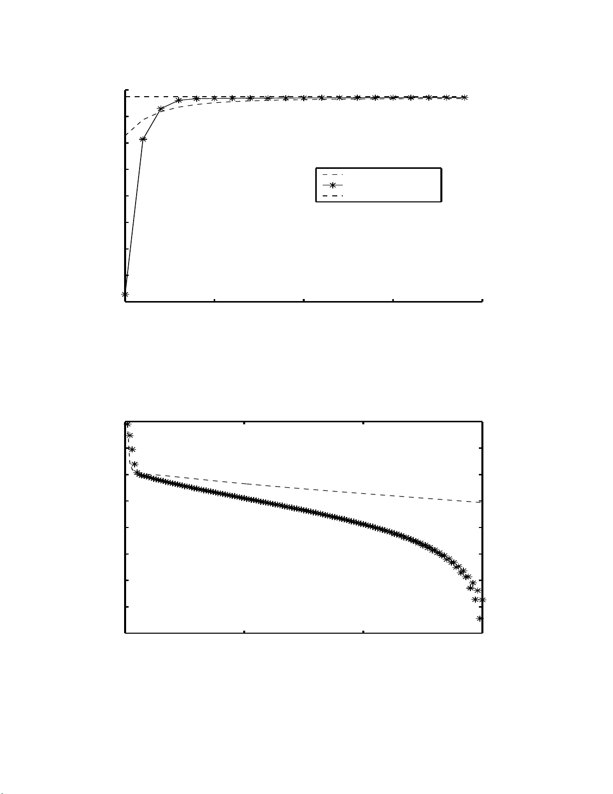
Kullbac k Pro ximal Algorithms for Maxim um Lik eliho o d Estimation ∗ St ´ ephane Chr´ etien, Alfred O. Hero Abstract Accelerat ed algorithms fo r maxim um lik elihoo d image reconstruction are essen- tial for emerging applicat ions suc h as 3D tomography , dynamic tomographic imag- ing, and other high dimensional inv e rse problems. In this pap er, we in tro duce and analyze a class of fast and stable sequential optimization m ethods for computing maxim um lik elihoo d estimates and study its con v ergence prop erties. These me tho ds are based on a pr oximal p oint algorithm implemen ted with the Kullbac k-Liebler (KL) div ergence b et w een p osterior densities of the complete data as a p ro ximal p en alt y function. When the pro ximal relaxation p arameter is set to u n it y one obtains the classical expectation maximization (EM) algorithm. F or a decreasing sequence of re- laxation parameters, relaxed v ersions of EM are obtained whic h can ha v e m uc h faster asymptotic con v ergence without sacrifice of monotonicit y . W e pr esen t an implemen- tation of the algorithm using Mor´ e’s T rust R e gion u p date strategy . F or illustr ation the metho d is applied to a n on-quadratic in v erse problem with Poisson distribu ted data. Keyw ords : ac c eler ate d EM algorithm, Ku l lb ack- Liebler r elaxation, pr oximal p oint iter ations, sup erline ar c onver genc e, T rust R e gion metho ds, emission tomo gr aphy. 1 Stephane Chretien is w ith Universit´ e Libre de Bruxelle s , Campus de la P la ine, CP 2 1 0-01, 1050 Bruxelles, Belgium, (schretie@smg.ulb.ac.b e) and Alfred Hero is with the Dept. of Electrical Engi- neering and Co mputer Science, 1301 Beal St., Universit y o f Michigan, Ann Arbo r, MI 4810 9-2122 (hero@eecs.umich.edu). This resear ch was supp orted in part b y AFOSR grant F49620 - 97-0028 1 LIST OF FIGURES 1. Tw o rail p han tom for 1D deblur ring example. 2. Blurred t wo lev el ph an tom. Blurr ing k ernel is Gaussian w ith standard width ap- pro ximately equ al to rail separation dista nce in phan tom. An ad d itiv e randoms noise of 0.3 w as added. 3. Snapshot of log–Lik elihoo d vs iteration for plain EM and KPP EM algorithm. Plain EM initially prod uces greater increases in lik eliho od function but is o ve r- tak en b y KPP EM at 7 iterations and thereafter. 4. The sequence log k θ k − θ ∗ k vs iteration for plain EM and KPP EM algorithms. Here θ ∗ is limiting v alue for eac h of the algorithms. Note the sup erlinear con- v ergence of K PP . 5. Reconstructed images after 150 iterations of plain EM and KPP E M algorithms. 6. Ev olution of the reconstructed sour ce vs iteration for p lain EM and KP P EM. 2 1 In tro ducti on Maxim um lik eliho od (ML) or maxim um p enalized lik eliho od (MPL) approac hes ha v e b een widely adopted for image restoration and image reconstruction from noise con- taminated data with known statistical distribution. In man y cases the likel iho o d function is in a form for whic h analytica l solution is d ifficult or imp ossible. When this is the case iterat iv e solutions to the ML reconstruction or restoration problem are of in terest. Among th e most stable iterativ e strategies for ML is th e p opular exp ectatio n maximizati on (EM) algorithm [8]. The EM algorithm has b een wid ely applied to emission and transmission compu ted tomograph y [39, 23, 36] with Po isson data. T h e EM algorithm has the attractiv e p rop ert y of monotonicit y w hic h guar- an tees that the lik elihoo d fu n ction increases with eac h iteration. The con v ergence prop erties of the EM algorithm and its v arian ts ha v e b een ext ensive ly stu died in t he literature; see [42] and [15] for instance. It is w ell known that under strong co nca vit y assumptions the EM algorithm conv erges linearly to w ards th e ML estimat or θ M L . Ho w ev er, the r ate co efficien t is small and in practice th e EM algo rithm suffers fr om slo w con v ergence in late iteratio ns. Efforts to improv e on the asymptotic con v ergence rate of the EM alg orithm h a ve included: Aitken’s acceleratio n [28], ov er-relaxation [26], conjugate gradien t [20] [19], Newton metho ds [30] [4], quasi-Newton methods [22], ordered subsets EM [17] and sto c hastic EM [25]. Unfortun ate ly , these metho ds do not automaticall y guarantee the monotone increasing likeli ho o d pr op er ty as do es standard EM. F u r thermore, many of these accelerated algorithms require additional monitoring for instabilit y [24]. T his is esp ecially problematic for high dimensional image reconstruction problems, e.g. 3D o r dynamic imaging, wh ere m onitoring could add signifi can t computational o v erhead to the reconstruction algorithm. The con tr ibution of this pap er is the in tro duction of a class of ac celerated EM algorithms f or lik eliho od function maximizat ion via exploit ation of a general relation b et w een EM and proxi mal p oin t (PP) alg orithms. Th ese algorithms con v erge and can h a v e qu ad r atic rates of conv ergence ev en with approximate up dating. Proximal p oin t algorithms w ere i ntrodu ced b y Martinet [29] and Ro c k afellar [38], based on the w ork of Mint y [31] and Moreau [33], for the p urp ose of s olving conv ex minimization problems with con v ex constraints. A ke y m otiv atio n for the PP algorithm is that b y add in g a sequence of iteration-dep endent p enalties, called pro ximal p enalties, to the o b jectiv e fu nction to b e maximized one obtains stable iterativ e al gorithms whic h frequent ly ou tp erf orm standard optimization metho ds w ith ou t pr oximal p enalties, e.g. see Goldstein and Russak [1]. F u rthermore, the PP algorithm pla ys a paramoun t role in non-differentia ble optimization due to its connections with the Mo reau-Y osida regularization; see Min t y [31], Moreau [33], Ro c k afellar [38] and Hiriart-Hurrut y and Lemar ´ ec hal [16]. While the original PP algorithm used a simple quadratic p enalt y more general v ersions of PP ha v e r ecently b een prop osed whic h use non-qu adratic p enalties, and in particular e nt ropic penalties. Suc h p enalties are most co mmonly applied to ensure non-negativit y when solving Lagrange duals of inequalit y constrained primal pr ob- lems; see f or examp le pap ers by Censor and Z enios [5 ], Eks tein [10 ], Eggermon t [9], and T ebou lle [40]. In this pap er w e sho w that by c ho osin g the pro ximal p enalt y 3 function of PP as the Kullbac k-Liebler (KL) div ergence b etw een successive iterates of the p osterior densities of the co mplete data, a generalizat ion of the generic E M maxim um lik elihoo d algorithm is obtained with acce lerated con v ergence rate. When the relaxation sequence is constan t and equal to un it y the PP algo rithm with KL pro ximal p enalt y redu ces to the stand ard EM algorithm. On the other hand f or a de- creasing relaxation sequence the PP algorithm with KL pr o ximal p enalt y is sho wn to yield an iterativ e ML algorithm whic h has m uc h faster conv ergence than EM without sacrificing its monotonic lik eliho od prop ert y . It is imp ortan t to p oin t out that relations b et wee n particular EM and particular PP algorithms ha v e b een previously observ ed, but not in the full generalit y estab- lished in this pap er. Sp ecifically , for parameters constrained to the non-n ega tiv e orthan t, Egg ermont [9] established a relation b et w een an en tropic mo dification of the standard PP algorithm and a class of m ultiplicativ e metho ds for smo oth con v ex optimization. Th e mo dified PP algorithm that was int ro duced in [9] was obtained b y r eplaci ng the standard quadratic p enal t y by the r ela tiv e ent ropy b et w een suc c es- sive non-ne gative p ar am eter iter ates . This extension was shown to b e equiv ale nt to an “implicit” algorithm wh ic h, after some appro ximations to the exact PP ob jecti v e function, reduces to the “explicit” Shepp and V ardi EM algorithm [39] for im age reconstruction in emission tomography . Egge rmont [9] wen t on to prov e that the explicit a nd implicit algorithms are monotonic and b oth c onv erge when the sequence of relaxation parameters is b oun ded b elo w by a strictly p ositive n umber. In con trast to [9], here w e establish a general and exa ct relati on b et w een the generic EM p rocedu re, i.e. arb itrary incomplete and complete data distributions, and an extended class of PP algorithms. As p ointed out ab o v e, the extended PP algorithm is implemente d with a p ro ximal p enalt y which is the relativ e ent ropy (KL div ergence) b et w een suc c essive iter ates of the p osterior densities of the c omplete data . This mo dification pro duces a class of algorithms whic h we r efer to as Kullbac k-Liebler pro ximal p oint (KPP). W e p r o v e a global con v ergence result for the KPP algorithm under strict conca vit y assumptions. An appr o x im ate KPP is also prop osed using the T ru st Region strategy [32, 34] adapted to KPP . W e show, in p articular, that b oth the exact and appr o xim ate KPP algorithms ha v e sup erlinear con v ergence rates when the s equence of p ositiv e relaxation parameters con v erge to zero. Finally , we illustrate these r esu lts for KPP accele ration of the Shepp and V ardi EM alg orithm implemen ted with T rust R egion u p dating. The results giv en here are also app lica ble to the non-linear up dating m ethods of K ivinen and W armuth [21] for accelerati ng the conv ergence of Gaussian mixture- mo del identi fication algorithms in sup ervised mac hine learning, see also W arm uth and Azo ury [41] and Helmbold, Sc hapire, Singer and W arm uth [14]. Indeed, simi- larly to the general K PP alg orithm in tro duced in this pap er, in [14] the KL diverge nce b et w een the n ew and the old mixtur e mo del w as added to the gradient of the Gaus- sian mixture-model lik elihoo d fu nction, ap p ropriately weig ht ed with a m ultiplicat iv e factor called the learnin g r ate parameter. T his pro cedu re le d to w hat the authors of [14] call ed an exp onen tiate d gradien t algorithm. These authors pro vided exp erimen- tal evidence of sig nificant imp r o v emen ts in con v ergence rate as compared to gradien t descen t and ordinary EM. Th e r esults in this pap er pr o vide a general theory whic h 4 v alidate suc h exp erimental results f or a very broad class of p arametric estimation problems. The outline of the pap er is as f ollo ws. In Section 2 we provide a brief r eview of k ey elemen ts of the classical EM alg orithm. In Section 3, w e establish the general relationship betw ee n the EM algo rithm and the pro ximal p o int algo rithm. In section 4, we present the general KPP algorithm and w e establish global and su p erlinear con v ergence to the maxim um likelihoo d estimator for a sm o oth and strictly conca v e lik elihoo d fu nction. In section 5, we study second order approximat ions of the KPP iteration using T rust Regio n up dating. Finally , in Section 6 w e presen t n umerical comparisons for a P oisson in v erse problem. 2 Bac kground The problem of maxim um lik eliho od (ML) estimation consists of fin ding a solution of the form θ M L = argmax θ ∈ R p l y ( θ ) , (1) where y is an observe d s ample of a random v ariable Y defined on a sample space Y and l y ( θ ) is the log-lik eliho od fun ctio n defined by l y ( θ ) = log g ( y ; θ ) , (2) and g ( y ; θ ) den ote s the density of Y at y p arametrize d b y a v ect or parameter θ in R p . O ne of the most p opular iterativ e m ethods for solving ML estimation p r oblems is the Exp ectati on Maximization (EM) algorithm describ ed in Dempster, Laird, and Rubin [8] which w e recall f or the reader. A more informativ e d ata space X is int ro duced. A rand om v ariable X is defined on X with densit y f ( x ; θ ) parametrized by θ . Th e data X is more inf ormativ e than the actual data Y in the sense that Y is a compression of X , i.e. there exists a non-in v ertible transformation h such that Y = h ( X ). If one had access to the data X it wo uld therefore b e adv an tage ous to replace the ML estimation p roblem (1) by ˆ θ M L = argmax θ ∈ R p l x ( θ ) , (3) with l x ( θ ) = log f ( x ; θ ). Sin ce y = h ( x ) the densit y g of Y is related to the d ensit y f of X thr ou gh g ( y ; θ ) = Z h − 1 ( { y } ) f ( x ; θ ) dµ ( x ) (4) for an appropr iate measure µ on X . In this setting, the data y are called inc omplete data wh ereas the data x are called c omp lete data . Of course the complete data x corresp onding to a giv en observ ed s ample y are unknown. Therefore, the complete data lik eliho o d fu nction l x ( θ ) can only b e es- timated. Give n the observed data y and a pr evious estimate of θ denoted ¯ θ , the 5 follo wing minimum mean square error estimator (MMSE) of the quan tit y l x ( θ ) is natural Q ( θ , ¯ θ ) = E [log f ( x ; θ ) | y ; ¯ θ ] , where, for any int egrable function F ( x ) on X , w e hav e d efined the conditional ex- p ectatio n E [ F ( x ) | y ; ¯ θ ] = Z h − 1 ( { y } ) F ( x ) k ( x | y ; ¯ θ ) dµ ( x ) and k ( x | y ; ¯ θ ) is the cond itio nal den s it y f u nction giv en y k ( x | y ; ¯ θ ) = f ( x ; ¯ θ ) g ( y ; ¯ θ ) . (5) The EM algorithm generates a sequ en ce of appro ximations to the solution (3 ) starting from an initial guess θ 0 of θ M L and is d efined b y Compute Q ( θ , θ k ) = E [log f ( x ; θ ) | y ; θ k ] E Step θ k +1 = argmax θ ∈ R p Q ( θ , θ k ) M Step A key to und er s tanding the con v ergence of the EM algorithm is th e decomp osi- tion of the lik eliho o d fu nction p resen ted in Dempster, Laird and Rub in [8]. As this decomp osition is also the prime motiv ation for the KPP generalization of EM it will b e worth while to recall certain eleme nts of their argumen t. The lik eliho od can b e decomp osed as l y ( θ ) = Q ( θ , ¯ θ ) + H ( θ , ¯ θ ) (6) where H ( θ , ¯ θ ) = − E [log k ( x | y ; θ ) | y ; ¯ θ ] . It follo ws from elemen tary application of Jensen’s inequalit y to the log function that H ( θ , ¯ θ ) ≥ H ( θ , θ ) ≥ 0 , ∀ θ , ¯ θ ∈ R p . (7) Observe from (6) a nd (7) that for an y θ k the θ function Q ( θ, θ k ) is a lo w er b ound on the log lik elihoo d fun ction l y ( θ ). This p rop ert y is sufficien t to ensu re monotonicit y of the algorithm. Sp ecifically , since the th e M-step implies that Q ( θ k +1 , θ k ) ≥ Q ( θ k , θ k ) , (8) one obtains l y ( θ k +1 ) − l y ( θ k ) ≥ Q ( θ k +1 , θ k ) − Q ( θ k , θ k ) (9) + H ( θ k +1 , θ k ) − H ( θ k , θ k ) . Hence, usin g (8) an d (7) l y ( θ k +1 ) ≥ l y ( θ k ) . This is the w ell kno wn monotonicit y prop ert y of the EM algorithm. Note that if the fu nction H ( θ , ¯ θ ) in (6) w ere scaled b y an arbitrary p ositiv e factor β the function Q ( θ , ¯ θ ) would remain a lo w er b ound on l y ( θ ), the r igh t hand side of (9) would remain positiv e and monotonicit y of the algorithm w ould b e preserv ed. As will b e sho wn b elo w , if β is allo we d to v ary w ith iteration in a suitable manner one obtains a monotone, sup erlinearly conv ergent generalizatio n of the EM algorithm. 6 3 Pro ximal p oin t m etho ds a nd the EM algo- rithm In this section, we presen t the pro ximal p oin t (PP) algorithm of Ro c k afellar and Martinet. W e then demonstrate that EM is a particular case of proximal point implemen ted with a Kullbac k-t yp e proximal p enalt y . 3.1 The pro ximal p oin t algorithm Consider the general pr oblem of maximizing a conca v e f unction Φ( θ ). The pro ximal p oin t algorithm is an iterativ e p r ocedur e whic h can b e wr itte n θ k +1 = argmax θ ∈ R p  Φ( θ ) − β k 2 k θ − θ k k 2  . (10) The quadratic p enalt y k θ − θ k k 2 is r elaxe d using a sequence of p ositiv e parameters { β k } . In [3 8], Ro c k afellar show ed that su p erlinear conv ergence of this method is obtained when the sequence { β k } con v erges to w ards zero. In n umerical implement a- tions of pro ximal p oin t the f unction Φ( θ ) is generally replaced b y a p iece wise linear mo del [16]. 3.2 Pro ximal in terpretat ion of the EM algorithm In th is section, we establish an exact relationship b et w een the generic EM pro ce- dure an d an extended p r o ximal p oint algorithm. F or our p urp oses, w e will need to consider a particular Kullbac k-Liebler (KL) information measure. Assu me that the family of conditional densities { k ( x | y ; θ ) } θ ∈ R p is regular in the sense of Ibragimo v and K hasminskii [18], in particular k ( x | y ; θ ) µ ( x ) and k ( x | y ; ¯ θ ) µ ( x ) are mutually ab- solutely con tin uous for an y θ and ¯ θ in R p . Then the Radon-Nik o dym deriv ativ e k ( x | y, ¯ θ ) k ( x | y ; θ ) exists f or all θ , ¯ θ and we can defin e the follo wing K L diverge nce: I y ( ¯ θ , θ ) = E  log k ( x | y , ¯ θ ) k ( x | y ; θ ) | y ; ¯ θ  . (11) Prop osition 1 The EM algorithm is e quivalent to the fol lowing r e cu rsion with β k = 1 , k = 1 , 2 , . . . , θ k +1 = argmax θ ∈ R p n l y ( θ ) − β k I y ( θ k , θ ) o (12) F or general p ositiv e sequence { β k } the recursion in Prop osition 1 can b e identi- fied as a mo dification of the PP algorithm (10) with the standard qu adratic p enalt y 7 replaced by the KL p enalt y (11) and ha ving relaxation sequence { β k } . In the se- quel we call this mo dified PP algorithm th e Ku llbac k-Liebler p ro ximal p oin t (KPP) algorithm. In many treatmen ts of the EM algorithm the quan tit y Q ( θ , ¯ θ ) = l y ( θ ) − l y ( ¯ θ ) − I ( ¯ θ , θ ) is the su rrogate fun ctio n that is maximized in the M-step. Th is surrogate ob j ec- tiv e function is identica l (up to an add itiv e constan t) to the KPP ob jectiv e l y ( θ ) − β k I y ( θ k , θ ) of (12) when β k = 1. Pr o of of Pr op osition 1: The k ey to making the conn ect ion with the proxima l p oint algorithm is the follo wing representa tion of th e M step: θ k +1 = argmax θ ∈ R p  log g ( y ; θ ) + E  log f ( x ; θ ) g ( y ; θ ) | y ; θ k  . This equation is equiv alent to θ k +1 = argmax θ ∈ R p  log g ( y ; θ ) + E  log f ( x ; θ ) g ( y ; θ ) | y ; θ k  − E  log f ( x ; θ k ) g ( y ; θ k ) | y ; θ k  since the additional term is constant in θ . Recall ing that k ( x | y ; θ ) = f ( x ; θ ) g ( y ; θ ) , θ k +1 = argmax θ ∈ R p  log g ( y ; θ ) + E  log k ( x | y ; θ ) | y ; θ k  − E  log k ( x | y ; θ k ) | y ; θ k  . W e fin ally obtain θ k +1 = argmax θ ∈ R p  log g ( y ; θ ) + E  log k ( x | y ; θ ) k ( x | y ; θ k ) | y ; θ k  whic h concludes the pro of.  4 Con v ergence of th e KPP A lgorithm In th is s ect ion we establish monotonicit y and other con v ergence prop erties of the KPP algorithm of Prop osition 1. 4.1 Monotonicit y F or b ound ed d omain of θ , the KPP algorithm is w ell defin ed since the maxim um in (12) is alw a ys achiev ed in a b ounded set. Monotonicit y is guaran teed b y this pro cedure as prov ed in the f ollo wing prop osition. 8 Prop osition 2 The lo g-likeliho o d se quenc e { l y ( θ k ) } is mono tone non-de cr e asing and satisfies l y ( θ k +1 ) − l y ( θ k ) ≥ β k I y ( θ k , θ k +1 ) , (13) Pr o of: F r om the recurrence in (12), we ha v e l y ( θ k +1 ) − l y ( θ k ) ≥ β k I y ( θ k , θ k +1 ) − β k I y ( θ k , θ k ) . Since I y ( θ k , θ k ) = 0 and I y ( θ k , θ k +1 ) ≥ 0, w e deduce (13) and th at { l y ( θ k ) } is n on- decreasing.  W e n ext turn to asymp totic con v ergence of the K PP iterates { θ k } . 4.2 Asymptotic Con v ergence In the sequel ∇ 01 I y ( ¯ θ , θ ) (resp ectiv ely ∇ 2 01 I y ( ¯ θ , θ )) denotes the gradien t (respective ly the Hessian matrix) of I y ( ¯ θ , θ ) in th e first v ariable. F or a square matrix M , Λ M denotes th e greatest eigen v alue of a matrix M and λ M denotes th e smallest. W e m ak e the follo wing assum ptions Assumptions 1 We assume the fol lowing: (i) l y ( θ ) is twic e c ontinuously d iffer entiable on R p and I y ( ¯ θ , θ ) is twic e c ontinuously differ entiable in ( θ , ¯ θ ) in R p × R p . (ii) lim k θ k→∞ l y ( θ ) = −∞ wher e k θ k is the stand ar d Euclide an norm on R p . (iii) l y ( θ ) < ∞ and Λ ∇ 2 l y ( θ ) < 0 on every b ounde d θ -set. (iv) for any ¯ θ in R p , I y ( ¯ θ , θ ) < ∞ and 0 < λ ∇ 2 01 I y ( ¯ θ , θ ) ≤ Λ ∇ 2 01 I y ( ¯ θ , θ ) on every b ounde d θ -set. These assu m ptions ensu re smo othness of l y ( θ ) and I y ( ¯ θ , θ ) and their fi rst t w o deriv at iv es in θ . Assu mption 1.iii also implies strong conca vit y of l y ( θ ). Assumption 1.iv implies that I y ( ¯ θ , θ ) is strictly c on ve x and that the parameter θ is s tr ongly iden tifiable in the family of densities k ( x | y ; θ ) (see pro of of Lemma 1 b elo w). Note that the ab o v e assumptions are not the minimum p ossible set, e.g. that l y ( θ ) and I y ( ¯ θ , θ ) are upp er b ounded follo ws fr om con tin uit y , Assumption 1.ii and the prop erty I y ( ¯ θ , θ ) ≥ I y ( ¯ θ , ¯ θ ) = 0, resp ectiv ely . W e fi rst c haracterize the fi xed p oin ts of the KPP algorithm. A r esult that w ill b e used rep eatedly in the sequel is that for any ¯ θ ∈ R p ∇ 01 I y ( ¯ θ , ¯ θ ) = 0 . (14) 9 This follo ws immediately from the inform ation inequalit y for the KL div ergence [7, Thm. 2.6.3 ] I y ( ¯ θ , θ ) ≥ I y ( ¯ θ , ¯ θ ) = 0 , so that, by smo othness Assum ption 1.i, I y ( ¯ θ , θ ) has a stationary p oint at θ = ¯ θ . Prop osition 3 L et the densities g ( y ; θ ) and k ( x | y ; θ ) b e such that Assumptions 1 ar e satisfie d. Then the fixe d p oints of the r e curr enc e in (12) ar e maximizers of the lo g-likeliho o d function l y ( θ ) for any r e laxa tion se quenc e β k = β > 0 , k = 1 , 2 , . . . . Pr o of: C onsider a fi xed p oin t θ ∗ of the recurrence relation (12) for β k = β = constant . Then, θ ∗ = argmax θ ∈ R p { l y ( θ ) − β I y ( θ ∗ , θ ) } . As l y ( θ ) and I y ( θ ∗ , θ ) are b oth s mooth in θ , θ ∗ m ust b e a stationary p oint 0 = ∇ l y ( θ ∗ ) − β ∇ 01 I y ( θ ∗ , θ ∗ ) . Th us, as by (14) ∇ 01 I y ( θ ∗ , θ ∗ ) = 0, 0 = ∇ l y ( θ ) . (15) Since l y ( θ ) is str ictl y conca v e, we dedu ce that θ ∗ is a maximizer of l y ( θ ).  The follo wing w ill b e useful. Lemma 1 L et th e c onditional density k ( x | y ; θ ) b e such that I y ( ¯ θ , θ ) satisfies Assump- tion 1.iv. Th en, giv en two b ounde d se quenc es { θ k 1 } and { θ k 2 } , lim k →∞ I y ( θ k 1 , θ k 2 ) = 0 implies that lim k →∞ k θ k 1 − θ k 2 k = 0 . Pr o of: Let B b e an y b ounded set con taining b oth sequences { θ k 1 } and { θ k 2 } . Let λ denote th e minimum λ = min θ , ¯ θ ∈B λ ∇ 2 01 I y ( ¯ θ ,θ ) (16) Assumption 1.iv implies that λ > 0. F urthermore, in v oking T aylo r’s theorem with remainder, I y ( ¯ θ , θ ) is strictly con v ex in the sense that for an y k I y ( θ k 1 , θ k 2 ) ≥ I y ( θ k 1 , θ k 1 )+ ∇ I y ( θ k 1 , θ k 1 ) T ( θ k 1 − θ k 2 ) + 1 2 λ k θ k 1 − θ k 2 k 2 . As I y ( θ k 1 , θ k 1 ) = 0 and ∇ 01 I y ( θ k 1 , θ k 1 ) = 0, recall (14), w e obtain I y ( θ k 1 , θ k 2 ) ≥ λ 2 k θ k 1 − θ k 2 k 2 . The d esired result comes from passing to the limit k → ∞ .  Using these results, we easily obtain the follo wing. 10 Lemma 2 L et the densities g ( y ; θ ) and k ( x | y ; θ ) b e such that Assumptions 1 ar e satisfie d. Then { θ k } k ∈ N is b ounde d. Pr o of: Due to Pr op osition 2, th e sequ en ce { l y ( θ k ) } is m onoto ne in cr easing. There- fore, assu mption 1.ii imp lies that { θ k } is b ounded .  In the follo wing lemma, w e prov e a r esult which is often called asymptotic r egu- larit y [2]. Lemma 3 L et the densities g ( y ; θ ) and k ( x | y ; θ ) b e such that l y ( θ ) and I y ( ¯ θ , θ ) satisfy Assumptions 1. L et the se que nc e of r elaxation p ar ameters { β k } k ∈ N satisfy 0 < lim inf β k ≤ lim sup β k < ∞ . Then, lim k →∞ k θ k +1 − θ k k = 0 . (17) Pr o of: By Assumption 1.iii and b y Prop osition 2 { l y ( θ k ) } k ∈ N is b ounded and monotone. Since, by Lemma 2 , { θ k } k ∈ N is a b ound ed s equence { l y ( θ k ) } k ∈ N con- v erges. Therefore, lim k →∞  l y ( θ k +1 ) − l y ( θ k )  = 0 whic h, from (13), implies that β k I y ( θ k , θ k +1 ) v anishes when k tends to in finit y . Since { β k } k ∈ N is boun ded b elo w b y lim inf β k > 0: lim k →∞ I y ( θ k , θ k +1 ) = 0. Therefore, Lemma 1 establishes the desired result.  W e can no w giv e a global conv ergence theorem. Theorem 1 L et the se quenc e of r elaxation p ar ameters { β k } k ∈ N b e p ositive and c on- ver ge to a limit β ∗ ∈ [0 , ∞ ) . Then the se quenc e { θ k } k ∈ N c onver ges to the solution of the ML estimation pr oblem (1). Pr o of: S ince { θ k } k ∈ N is bou n ded, one can extract a conv er gent subsequence { θ σ ( k ) } k ∈ N with limit θ ∗ . T he defining recurrence (12) imp lies that ∇ l y ( θ σ ( k )+1 ) − β σ ( k ) ∇ 01 I y ( θ σ ( k ) , θ σ ( k )+1 ) = 0 . (18) W e no w p r o v e that θ ∗ is a stat ionary p oin t of l y ( θ ). Assume fi rst that { β k } k ∈ N con v erges to zero, i.e. β ∗ = 0. Due to Assump tions 1 .i, ∇ l y ( θ ) is co nt inuous in θ . Hence, since ∇ 01 I y ( ¯ θ , θ ) is b ounded on b ounded su bsets, (18) im p lies ∇ l y ( θ ∗ ) = 0 . Next, assume that β ∗ > 0. In this case, Lemma 3 establishes that lim k →∞ k θ k +1 − θ k k = 0 . 11 Therefore, { θ σ ( k )+1 } k ∈ N also tends to θ ∗ . S ince ∇ 01 I y ( ¯ θ , θ ) is conti nuous in ( ¯ θ , θ ) equation (18) giv es at infinity ∇ l y ( θ ∗ ) − β ∗ ∇ 01 I y ( θ ∗ , θ ∗ ) = 0 . Finally , by (14), ∇ 01 I y ( θ ∗ , θ ∗ ) = 0 and ∇ l y ( θ ∗ ) = 0 . (19) The pro of is concluded as follo ws. As, by Assumption 1.iii, l y ( θ ) is conca v e, θ ∗ is a maximizer of l y ( θ ) so that θ ∗ solv es the Maximum Like liho o d estimation pr oblem (1). F urthermore, as p ositiv e definiteness of ∇ 2 l y implies that l y ( θ ) is in fact s trictly conca v e, this ma ximizer is un ique. Hence, { θ k } h as only one accumulat ion p oin t and { θ k } conv erge s to θ ∗ whic h ends th e pro of.  W e no w establish the main result concerning sp eed of con v ergence. Recall that a sequence { θ k } is said to con v erge s u p erlinearly to a limit θ ∗ if: lim k →∞ k θ k +1 − θ ∗ k k θ k − θ ∗ k = 0 , . (20) Theorem 2 Assume that the se quenc e of p ositive r elaxation p ar ameters { β k } k ∈ N c onver ges to zer o. Then, the se quenc e { θ k } k ∈ N c onver ges sup erline arly to the solutio n of the ML estimation pr oblem (1). Pr o of: Due to Theorem 1, the sequence { θ k } con v erges to the unique m aximize r θ M L of l y ( θ ). Assu mption 1.i implies that the g radient mapping ∇ θ  l y ( θ ) − β k I y ( θ M L , θ )  is con tin uously differen tiable. He nce, w e hav e the f ollo wing T a ylor expansion ab out θ M L . ∇ l y ( θ ) − β k ∇ 01 I y ( θ M L , θ ) = ∇ l y ( θ M L ) − β k ∇ 01 I y ( θ M L , θ M L ) + ∇ 2 l y ( θ M L )( θ − θ M L ) (21) − β k ∇ 2 01 I y ( θ M L , θ M L )( θ − θ M L ) + R ( θ − θ M L ) , where th e remainder satisfies lim θ → θ M L k R ( θ − θ M L ) k k θ − θ M L k = 0 . Since θ M L maximizes l y ( θ ), ∇ l y ( θ M L ) = 0. F urthermore, by (14), ∇ 01 I y ( θ M L , θ M L ) = 0. Hence, (21) can b e simplified to ∇ l y ( θ ) − β k ∇ 01 I y ( θ M L , θ ) = ∇ 2 l y ( θ M L )( θ − θ M L ) − β k ∇ 2 01 I y ( θ M L , θ M L )( θ − θ M L ) + R ( θ − θ M L ) . (22) 12 F r om the definin g relation (12) the iterate θ k +1 satisfies ∇ l y ( θ k +1 ) − β k ∇ 01 I y ( θ k , θ k +1 ) = 0 . (23) So, taking θ = θ k +1 in (22 ) and u sing (23), we obtain β k  ∇ 01 I y ( θ k , θ k +1 ) − ∇ 01 I y ( θ M L , θ k +1 )  = + ∇ 2 l y ( θ M L )( θ k +1 − θ M L ) − β k ∇ 2 01 I y ( θ M L , θ M L )( θ k +1 − θ M L ) + R ( θ k +1 − θ M L ) . Th us, k β k  ∇ 01 I y ( θ k , θ k +1 ) − ∇ 01 I y ( θ M L , θ k +1 )  − R ( θ k +1 − θ M L ) k = k∇ 2 l y ( θ M L )( θ k +1 − θ M L ) − β k ∇ 2 01 I y ( θ M L , θ M L )( θ k +1 − θ M L ) k . (24) On the other h and, one dedu ces from Assu mptions 1 (i) that ∇ 01 I y ( ¯ θ , θ ) is lo cally Lipsc hitz in the v ariables θ and ¯ θ . Then, since, { θ k } is b ounded, there exists a b ounded set B con taining { θ k } and a finite constan t L su c h that for all θ , θ ′ , ¯ θ and ¯ θ ′ in B , k∇ 01 I y ( ¯ θ , θ ) − ∇ 01 I y ( ¯ θ ′ , θ ′ ) k ≤ L  k θ − θ ′ k 2 + k ¯ θ − ¯ θ ′ k 2  1 2 . Using the triangle inequalit y and this last result, (24) asserts th at for any θ ∈ B β k L k θ k − θ M L k + k R ( θ k +1 − θ M L ) k ≥ k  ∇ 2 l y ( θ M L ) − β k ∇ 2 01 I y ( θ M L , θ M L )  ( θ k +1 − θ M L ) k . (25) No w, consider again the b ounded set B con taining { θ k } . L et λ l y and λ I denote the minima λ l y = min θ ∈B  − λ ∇ 2 l y ( θ )  λ I = min θ , ¯ θ ∈B n λ ∇ 2 01 I y ( ¯ θ , θ ) o . Since for any symmetric matrix H , x T H x/ k x k 2 is lo w er b ounded b y the minimum eigen v alue of H , w e h a v e immediately that k  −∇ 2 l y ( θ M L ) + β k ∇ 2 01 I y ( θ M L , θ M L )  ( θ k +1 − θ M L ) k 2 ≥  λ l y + β k λ I  2 k θ k +1 − θ M L k 2 . (26) By Assumptions 1.iii and 1.iv, λ l y + β k λ I > 0 and, after su bstitution of (26) in to (25), we obtain β k L k θ k − θ M L k + k R ( θ k +1 − θ M L ) k ≥  λ l y + β k λ I  k θ k +1 − θ M L k , (27) for all θ ∈ B . Therefore, collecting terms in (27 ) β k L ≥  λ l y + β k λ I − k R ( θ k +1 − θ M L ) k k θ k +1 − θ M L k  k θ k +1 − θ M L k k θ k − θ M L k . (28) No w, r eca ll that { θ k } is con v ergen t. Thus, lim k →∞ k θ k − θ M L k = 0 and subsequen tly , lim k →∞ k R ( θ k +1 − θ M L ) k k θ k +1 − θ M L k = 0 d u e to th e definition of the remainder R . Finally , as β k con v erges to zero, L is b ounded and λ l y > 0, equation (28) giv es (20) with θ ∗ = θ M L and th e pro of of sup erlinear conv ergence is completed.  13 5 Second ord er Appro ximations and T rust Re- gion tec hniques The m aximiza tion in the KPP recursion (12) will not generally yield an explicit exact recursion in θ k and θ k +1 . T h us implement ation of the K PP algorithm metho ds may require line searc h or one-step-late app ro ximatio ns similar to th ose used f or the M- step of the non-explicit p enalized EM maximum lik eliho o d algorithm [13]. In this section, we d iscu ss an alternativ e whic h uses second ord er f u nction app ro ximatio ns and preserv es th e conv ergence prop erties of KPP esta blished in the p revious section. This second order sc heme is related to the w ell-kno wn T rust Region tec hnique for iterativ e optimization intro d uced by Mor ´ e [32]. 5.1 Appro ximate mo dels In order to obtain computable iterations, th e follo wing second order appro ximations of l y ( θ ) and I y ( θ k , θ ) are introduced ˆ l y ( θ ) = l y ( θ k ) + ∇ l y ( θ k ) T ( θ − θ k ) + 1 2 ( θ − θ k ) T H k ( θ − θ k ) . and ˆ I y ( θ , θ k ) = 1 2 ( θ − θ k ) T ∇ 2 01 I k ( θ − θ k ) . In the follo wing, we adopt the sim p le notation g k = ∇ l y ( θ k ) (a column v ecto r). A natural choic e for H k and I k is of course H k = ∇ 2 l y ( θ k ) and I k = ∇ 2 01 I y ( θ k , θ k ) . The app ro ximate KPP algorithm is defin ed as θ k +1 = argmax θ ∈ R p  l y ( θ k ) + g k ( θ − θ k ) + 1 2 ( θ − θ k ) T H k ( θ − θ k ) (29) − β k 2 ( θ − θ k ) T I k ( θ − θ k )  A t this p oint it is imp ortan t to make sev eral commen ts. Notice fir s t that for β k = 0, k = 1 , 2 , . . . , and H k = ∇ 2 l y ( θ k ), the app ro ximate step (29) is equiv alen t to a Newton step. It is w ell known that Newton’s metho d, al so kno wn as Fisher scoring, has sup erlinear asymptoti c con v ergence rate bu t ma y div erge if not p rop erly initialized. Therefore, at lea st for small v alues of the relaxat ion parameter β k , the appro ximate P P A algorithm m a y f ail to con v erge for reasons analogous in Newton’s 14 metho d [37]. On the other hand, for β k > 0 the term − β k 2 ( θ − θ k ) T I k ( θ − θ k ) p enalize s the distance of the next iterate θ k +1 to the current iterate θ k . Hence, w e can inte rpr et this term as a regularization or relaxatio n whic h stabilizes the p ossib ly diverge nt Newton algorithm without s acrificing its sup erlinear asymptotic con v ergence rate. By appropr iat e c hoice of { β k } the iterate θ k +1 can b e forced to remain in a regio n around θ k o v er whic h the quadratic mo del ˆ l y ( θ ) is accurate [32][3]. In ma ny cases a quadratic appro ximation of a single one of the tw o terms l y ( θ ) or I y ( θ k , θ ) is sufficien t to obtain a closed form for the maxim um in the KPP recursion (12). Naturally , when feasible, suc h a reduced appro ximation is preferable to the ap- pro ximation of both term s discussed ab o v e. F or concreteness, in the sequel, although our results hold for the redu ced approximat ion also , w e only pro v e con v ergence for the pr oximal p oin t algorithm imp lemented with the full tw o-t erm ap p ro ximation. Finally , note that (29) is quadratic in θ and the minimization problem clearly reduces to solving a linear system of equations. F or θ of mo derate dimen sion, these equations can b e efficien tly solv ed using conjugate gradient tec h niques [34]. Ho w- ev er, when the v ector θ in (29 ) is of large dimension, as frequently o ccurs in in ve rse problems, l imited memory BF GS quasi-Ne wton sc hemes for upd ating H k − β k I k ma y b e computationally m uc h more effici en t, see for example [34], [35], [27], [12] and [11]. 5.2 T rust Region Up date Strategy The T rust Region strategy pro ceeds as follo ws. The m odel ˆ l y ( θ ) is maximized in a ball B ( θ k , δ ) =  k θ − θ k k I k ≤ δ  cen tered at θ k where δ is a proximit y con trol parameter whic h ma y depen d on k , and where k a k I k = a T I k a is a norm ; well defined due to p ositiv e definiteness of I k (Assumption 1.iv). Giv en an iterate θ k consider a candidate θ δ for θ k +1 defined as the solution to the constrained optimization p roblem θ δ = argmax θ ∈ R p ˆ l y ( θ ) sub ject to k θ − θ k k I k ≤ δ. (30) By duality theory of constrained optimization [16], and the fact that ˆ l y ( θ ) is strictly conca v e, this p roblem is equiv alen t to the un constrained optimizat ion θ δ ( β ) = argmin θ ∈ R p L ( θ , β ) . (31) where L ( θ , β ) = − ˆ l y ( θ ) + β 2  k θ − θ k k 2 I k − δ 2  . and β is a Lagrange m ultiplier selected to meet the constrain t (30) w ith equalit y: k θ δ ( β ) − θ k I k = δ . W e conclude that the T rust Region candid ate θ δ is id en tica l to the appro ximate KPP iterate (29 ) with relaxation parameter β c hosen according to constrain t (30). This relatio n also provides a rational rule for computing the r ela xation parameter β . 15 5.3 Implemen tat ion The p arameter δ is said to b e safe if θ δ pro duces an acceptable increase in the original ob jectiv e l y . An iteration of the T rust Regio n metho d consists of t wo principal steps R ule 1 . Determine wh ether δ is safe or not. If δ is safe, set δ k = δ and take an appro ximate Kullbac k proximal step θ k +1 = θ δ . Otherwise, tak e a nul l step θ k +1 = θ k . R ule 2 . Up d ate δ d ep en ding on the result of Rule 1 . Rule 1 can b e implemen ted b y comparing the increase in the original log-lik eliho o d l y to a fracti on m of the e xp ected increase predicted by the appro ximate model ˆ l y ( θ ). Sp ecifically , the T rust Region parameter δ is accepted if l y ( θ δ ) − l y ( θ k ) ≥ m  ˆ l y ( θ δ ) − ˆ l y ( θ k )  . (32) Rule 2 can b e implemented as follo ws. If δ was acc epted by Rule 1, δ is increased at the next iteration in order to exte nd the region of v alidit y of the mo del ˆ l y ( θ ). If δ w as rejected, the region must b e t igh tened and δ is d ecrea sed at the next iteration. The T rust Region strategy implement ed here is essentia lly the same as that p ro- p osed b y Mor ´ e [32]. Algorithm 1 Step 0. (Initialization) Set θ 0 ∈ R p , δ 0 > 0 and the “curve se ar ch” p ar ameters m , m ′ with 0 < m < m ′ < 1 . Step 1. With ˆ l y ( θ ) the qu adr atic appr oximation (29), solve θ δ k = argmax θ ∈ R p ˆ l y ( θ ) subje ct to k θ − θ k k I k ≤ δ k . Step 2. If l y ( θ δ k ) − l y ( θ k ) ≥ m  ˆ l y ( θ δ k ) − ˆ l y ( θ k )  then set θ k +1 = θ δ k . Otherwise, set θ k +1 = θ k . Step 3. Set k = k + 1 . Up date the mo del ˆ l y ( θ k ) . Up date δ k using Pr o c e dur e 1. Step 4. Go to Step 1. The p rocedu re for up dating δ k is giv en b elo w. Pro cedure 1 Step 0. (Initializatio n) Set γ 1 and γ 2 such that γ 1 < 1 < γ 2 . Step 1. If l y ( θ δ k ) − l y ( θ k ) ≤ m  ˆ l y ( θ δ k ) − ˆ l y ( θ k )  then take δ k +1 ∈ (0 , γ 1 δ k ) . 16 Step 2. If l y ( θ δ k ) − l y ( θ k ) ≤ m ′  ˆ l y ( θ δ k ) − ˆ l y ( θ k )  then take δ k +1 ∈ ( γ 1 δ k , δ k ) . Step 3. If l y ( θ δ k ) − l y ( θ k ) ≥ m ′  ˆ l y ( θ δ k ) − ˆ l y ( θ k )  then take δ k +1 ∈ ( δ k , γ 2 δ k ) . The T rust Region algorithm satisfies the follo wing con v ergence theorem Theorem 3 L et g ( y ; θ ) and k ( x | y ; θ ) b e such that Assumptions 1 ar e satisfie d. Then, { θ k } gener ate d b y A lgorithm 1 c onver ges to the maximizer θ M L of the lo g-likeliho o d l y ( θ ) and satisfies the monotone likeliho o d pr op erty l y ( θ k +1 ) ≥ l y ( θ k ) . If in ad di- tion, the se quenc e of L agr ange multipliers { β k } tends towar ds zer o, { θ k } c onver ges sup erline arly. The pr oof of Theorem 3 is omitted since it is standard in th e analysis of T ru st Region metho ds; see [32, 34]. Sup erlinear con v ergence for the case that lim k →∞ β k = 0 follo ws from the Dennis and Mor ´ e criterion [3, Theorem 3.11]. 5.4 Discussion The conv ergence results of Theorems 1 and 2 apply to any class of ob ject iv e fu nctions whic h satisfy the Assu mptions 1. F or instance, the analysis directly app lies to the p enalized maximum lik elihoo d (or p osterior lik eliho od ) ob jective f u nction l ′ y ( θ ) = l y ( θ ) + p ( θ ) when the ML p enalt y fu nction (prior) p ( θ ) is quadratic a nd non-negativ e of the form p ( θ ) = ( θ − θ o ) T R ( θ − θ o ), w h ere R is a non-negativ e definite matrix. The conv erge nce Th eorems 1 and 2 mak e u se of conca vit y of l y ( θ ) and conv exity of I y ( ¯ θ , θ ) via Assumptions 1.iii and 1.iv. How ever, for smo oth non-con v ex fun ctio ns an analogous lo cal su p erlinear con v ergence r esult can b e established und er some- what stronger assumptions s im ilar to those used in [15]. Lik ewise the T r u st Region framew ork can also b e applied to nonconv ex ob ject iv e functions. I n this case, global con v ergence to a lo cal maximizer of l y ( θ ) can b e established under Assumptions 1.i, 1.ii and 1.iv follo wing the p ro of tec hn ique of [32]. 6 Applicatio n to P oisson data In this section, w e illustrate th e ap p licat ion of Algo rithm 1 for a maximum lik elihoo d estimation p roblem in a Poisson inv erse p r oblem arising in r adiog raphy , thermionic emission pr ocesses, photo-detection, and p ositron emission tomograph y (PET). 17 6.1 The P oisson In v erse Problem The ob jectiv e is to estimate the int ensit y v ector θ = [ θ 1 , . . . , θ p ] T go v erning the n um- b er of gamma-ra y emissions N = [ N 1 , . . . , N p ] T o v er an imaging vol ume of p p ixels. The estimate of θ m ust be based on a vect or of m observed p r o jections of N denoted Y = [ Y 1 , . . . , Y m ] T . T h e comp onents N i of N are indep endent P oisson distribu ted with rate parameters θ i , and the comp onen ts Y j of Y are ind ep end en t Po isson d is- tributed with rate p aramete rs P p i =1 P j i θ i , where P j i is the transition p robabilit y; the probability that an emission from pixel i is detected at detector mo du le j . The standard choic e of complete d ata X , in trod uced b y S h epp and V ardi [39], for the EM algorithm is the set { N j i } 1 ≤ j ≤ m, 1 ≤ i ≤ p , where N j i denotes the num b er of emissions in pixel i whic h are detected at d etec tor j . The co rresp ond ing man y-to-one mapping h ( X ) = Y in the EM algorithm is Y j = p X i =1 N j i , 1 ≤ j ≤ m. (33) It is also w ell kn o wn [39] that th e lik elihoo d function is giv en by log g ( y ; θ ) = m X j =1  p X i =1 P j i θ i  − y j log  p X i =1 P j i θ i  + log y j ! (34) and th at the exp ectati on step of the EM algorithm is (see [13]) Q ( θ , ¯ θ ) = E [log f ( x ; θ ) | y ; ¯ θ ] = (35) m X j =1 p X i =1  y j P j i ¯ θ i P p i =1 P j i ¯ θ i log( P j i θ i ) − P j i θ i  . Let u s mak e th e follo wing additional assumptions: • the solution(s) of the Po isson inv erse pr oblem is (are) p ositiv e • the lev el s et L = { θ ∈ R n | l y ( θ ) ≥ l y ( θ 1 ) } (36) is b ounded and included in the p ositiv e orthant. Then, since l y is cont inuous, L is compact. Due to th e monotonicit y prop ert y of { θ k } , we thus dedu ce that for all k , θ k i ≥ γ for some γ > 0. Then, the lik eliho od function and the regularization function are b oth twice con tin uously differentia ble on the closure of { θ k } and the theory dev elop ed in this p ap er applies. These assumptions are ve ry close in spirit to the assumptions in Hero and F essler [15], except that w e do not require the maximizer to b e unique. The study of KPP w ithout these assump tions requires f urther analysis and is addressed in [6]. 18 6.2 Sim ulatio n results F or illustration w e p erformed numerical optimization for a simple one dimen sional deblurrin g example und er the P oisson noise mo del of the previous secti on. This example easily generalizes to more general 2 and 3 dimensional P oisson deblurring, tomographic reconstruction, and other imaging applications. T he true source θ is a tw o rail ph an tom sho wn in Figure 1. The blurring k ernel is a Gaussian function yielding the blurred ph antom sho wn in Figure 2. W e imp lemen ted b oth EM an d KPP with T rust Region up date strategy for deblur ring Fig. 2 when the set of ideal b lurred data Y i = P N j =1 P ij θ j is a v ailable without Poisson noise . In t his simple noiseless case the ML solution is equal to th e true source θ which is ev erywhere p ositiv e. T reatmen t of this noiseless case allo ws us to in v estigat e the b eha vior of the al gorithms in the asymptotic h igh coun t rate regime. More extensiv e sim ulatio ns with P oisson noise will b e p resen ted elsewhere. The numerical results sho wn in Fig. 3 indicate that the T rus t R egion imple- men tation of the KPP algorithm enjoys significant ly faster conv ergence to w ards th e optim um than d oes EM. F or th ese simulat ions the T rust Region tec hnique was imple- men ted in the standard m an n er wh ere the trust region size sequence δ k in Alg orithm 1 is determined implicitly by the β k up date rule: β k +1 = 1 . 6 β k ( δ k is decreased) and otherwise β k +1 = 0 . 5 β k ( δ k is increased). Th e resu lts sho wn in Fig. 4 v alidate the theoretical s u p erlinear conv ergence of the T rust Reg ion iterates as con trasted w ith the linear conv ergence rate of the EM iterates. Figure 5 sh o w s the reconstructed pr o- file and demonstrate s that the T ru st Reg ion up dated KPP te c hnique ac hiev es b et ter reconstruction of the original phan tom for a fixed n um b er of iterations. Finally , Figure 6 shows the iterates f or th e reconstru cte d phanto m, plotted as a fun ction of iteration on the horizon tal axis and as a fu nction of grey level on the v ertical axis. Observe t hat th e KPP ac hiev es more rapid separation of the tw o comp onen ts in the phant om th an do es standard EM. 7 Conclus ions The main con tributions of th is pap er are the follo wing. First, w e introd uced a general class of ite rativ e metho ds for ML estimati on based on Kullbac k-Liebler relaxation of the pr oximal p oint strategy . Next , we prov ed th at the EM algorithm b elongs to the prop osed class, th us pro viding a new and useful in terpretation of the EM app roac h for ML estimation. Finally , w e s ho w ed that Kullback proxima l p oin t metho ds enjo y global con v ergence and ev en sup erlinear con v ergence for sequences of p ositiv e r elax- ation parameters that con v erge to zero. Imp lementat ion issues w ere also discussed and we pr oposed second order sc hemes for the case w here the maximizatio n step is hard to obtain in closed form. W e addressed T rust Region metho dologies for th e up dating of the relaxatio n parameters. Compu tati onal exp erimen ts indicated that the a ppr o ximate second order KPP is stable and v erifi es t he sup erlinear c on v ergence prop ert y as w as predicted by our analysis. 19 References [1] A. A. Goldstein and I. B. Ru ssak, “Ho w go o d are the pro ximal p oin t algo- rithms?,” Numer. F unct. Ana l. and Optimiz. , vo l. 9, no. 7-8 , p p. 709–724, 1987. [2] H. H. Bausc hk e an d J. M. Borw ein, “On p r o jection algorithms for solving con v ex feasibilit y problems,” SIAM R evi ew , v ol. 38, n o. 3, pp. 367–426 , 1996. [3] J. F. Bonnans, J.-C. Gilbert, C. Lemar´ ec hal, and C. Sagasti zabal, O ptimiza tion num ´ erique . Asp e cts th ´ eoriques et pr atiques , vo lume 27, Springer V erlag, 1997. Series : Math´ ematiques et Applications. [4] C. Bouman and K. Sauer, “F ast n umerical methods for emission and trans- mission tomographic reconstruction,” in Pr o c. Conf. on Inform. Scienc es and Systems , John s Hopkins, 1993. [5] Y. Censor and S. A. Zenios, “Pro ximal m in imizat ion algorithm with D- functions,” Journ. O ptim. The ory and Appl. , vol . 73, no. 3, pp . 451–46 4, June 1992. [6] S. Chr´ etien and A. Hero, “Generalized pro ximal p oin t algorithms,” SIAM Journ. on Optimization , Sub mitted Sept., 1998. [7] T. Co v er and J . Thomas, Elements of Information The ory , Wiley , New Y ork, 1987. [8] A. P . Dempster, N. M. Laird, and D. B. Rubin, “Maxim um like liho o d f rom incomplete data via the EM algorithm,” J. R oyal Statistic al So ciety, Ser. B , v ol. 39, no. 1, pp. 1–38, 1977. [9] P . E gge rmont, “Multiplicativ e iterativ e algorithms for con v ex programming.,” Line ar Algebr a Appl. , v ol. 130, pp. 25–42, 1990. [10] J. Ekstein, “Nonlinear pro ximal p oin t algo rithms u sing Bregman fun ctions, with applications to con v ex p rogramming,” Math. Op er. R es. , v ol. 18, no. 1, pp. 203– 226, F ebruary 1993. [11] R. Fletc her, “A new v ariatio nal result for qu asi-Ne wton form ulae.,” SIAM J. Optim. , vol. 1, no. 1, pp. 18–21, 1991. [12] J. C. Gilb ert and C. Lemarec hal, “Some numerical exp erimen ts with v ariable- storage qu asi-Newton algorithms.,” Math. P r o gr am., Ser. B , v ol. 45, no. 3, pp. 407–4 35, 1989 . [13] P . J. Green, “On the use of the EM algorithm f or p enalized likelihoo d estima- tion,” J. R oya l Statistic al So ciety, Ser. B , vo l. 52, no. 2, pp . 443 –452, 1990. [14] D. Helm b old, R. Sc hapire, S. Y., and W. M., “A comparison of new and old algorithms for a mixture estimation problem,” Journal of Machine L e arning , v ol. 27, no. 1, pp. 97–119, 1997. [15] A. O. Hero and J. A. F essler, “Con v ergence in norm for alternating e xp ectation- maximization (EM) t yp e algo rithms,” Statistic a Sinic a , v ol. 5, n o. 1, pp. 41– 54, 1995. [16] J. B. Hiriart-Hurr ut y and C. L emar´ ec hal, Convex analysis and minimization algorithms I- II , Springer-V erlag, Bonn, 1993. 20 [17] H. Hudson and R. Larkin, “Ac celerated image reconstruction using ordered sub- sets of pr o jection data,” IEE E T r ansa ctions on Me dic al Ima ging , v ol. 13, no. 12, pp. 601–609, 1994. [18] I. A. Ib ragimo v and R. Z. Has’minskii, Statistic al estimation: Asymptotic the ory , Springer-V erlag, New Y ork, 1981. [19] M. J amshidian and R. I. Jennrich, “Conjugate gradien t acceleration of the EM algorithm,” J . Am. Statist. Asso c . , vo l. 88, no. 421, pp. 221–2 28, 1993 . [20] L. Kauf man, “Implementing and accelerating the EM algorithm for p ositron emission tomograph y ,” IEEE T r ans. on Me dic al Imaging , v ol. MI-6, no. 1, pp . 37–51 , 1987 . [21] J. Kivinen and M. K. W armuth, “Additiv e v ersus exp onen tiate d gradient up- dates for linear prediction,” Information and Computation , v ol. 132, pp. 1–64 , Jan uary 1997. [22] K. Lange, “A quasi-newtonian acceleratio n of the EM algorithm,” Statistic a Sinic a , vo l. 5, no. 1, pp. 1–18, 1995. [23] K. Lange and R. Carson, “EM r eco nstru ctio n algorithms for emission and tran s - mission tomograph y ,” Journal of Computer Assiste d T omo gr ap hy , vol. 8, n o. 2, pp. 306–316, April 1984. [24] D. Lansky an d G. Casella, “Imp ro ving the EM al gorithm,” in Computing and Statistics: Pr o c. Symp. on the Interfac e , C. Pag e and R. LeP ag e, editors, pp. 420–4 24, Springer-V erlag, 1990. [25] M. La vielle, “S to c hastic algorithm for parametric and non-parametric estimation in the case of incomplete d ata, ” Signal Pr o c essing , v ol. 42, no. 1, pp. 3–17 , 1995. [26] R. Lewitt and G. Mueh llehner, “Accelerated iterativ e reconstruction for p ositron emission tomograph y ,” IEEE T r ans. on Me dic al Imaging , v ol. MI-5, no. 1, pp . 16–22 , 1986 . [27] D. C. Liu and J. No cedal, “On the limited memory B F GS metho d for large scale optimization.,” M ath. Pr o gr am., Ser. B , vo l. 45, no. 3, pp . 503 –528, 1989. [28] T. A. Louis, “Finding the observ ed information matrix when using the EM algorithm,” J. R oyal Statistic al So ciety, Ser. B , vo l. 44, no. 2, pp. 226–233 , 1982. [29] B. Martinet, “R ´ egularisation d ’in ´ equation v ariationnelles par appro ximations successiv es,” R evue F r anc aise d’Informatique et de R e cher che Op er atio nnel le , v ol. 3, p p. 154– 179, 1970. [30] I. Meilijson, “A fast improv ement to the EM algo rithm on its own term s ,” J . R oyal Statistic al So c iety, Ser. B , vo l. 51, no. 1, pp . 127–1 38, 1989. [31] G. J . Min t y , “Monotone (non lin ear) op erators in Hilb ert space,” Duke Math. Journal , v ol. 29, pp. 341–3 46, 196 2. [32] J. J. Mor ´ e, “Recen t devel opments in algorithms and softw are for trust region metho ds,” in Mathematic al pr o gr amming: the state of the art , pp . 25 8–287, Springer-V erlag, Bonn, 1983. [33] J. J. Moreau, “Pro ximit ´ e et dualit ´ e dans u n espace Hilb ertien,” Bul l. So c. Math. F r anc e , v ol. 93, pp. 273–29 9, 1965. 21 [34] J. No cedal and S . J. W r igh t, Numeric al optimization , S p ringer Series in Op era- tions R esearch, Spr inger V erlag, Berlin, 1999. [35] J. No cedal, “Up dating quasi-Ne wton matrices with l imited sto rage.,” Math. Comput. , v ol. 35, pp. 773–7 82, 198 0. [36] J. M. Ollinger and D. L. Snyder, “A preliminary ev aluati on of the use of the EM algorithm for estimat ing p arameters in dyn amic tracer studies,” IEEE T r ans. Nucle ar Scienc e , v ol. NS-32, pp . 3575–35 83, F eb. 1985. [37] J. M. Ortega and W. C. Rh ein b oldt, Iter ative Solutio n of Nonline ar Equations in Sever al V ariables , Academic Press, New Y ork, 1970. [38] R. T. Ro c k afellar, “Monotone op erators and the proximal p oin t algorithm,” SIAM Journal on Contr ol and Optimization , v ol. 14, pp . 877–8 98, 1976 . [39] L. A. Shepp and Y. V ardi, “Maxim um lik eliho o d reconstruction for emission tomograph y ,” IEEE T r ans. on Me dic al Imaging , vol. MI-1, No. 2, p p. 113–122, Oct. 1982. [40] M. T eb oulle, “Entropic pro ximal mappings w ith application to nonlinear pro- gramming,” M athematics of O p er ations R ese ar ch , v ol. 17, pp . 670 –690, 1992. [41] M. W armuth and K. Azoury , “Relativ e loss b ounds for on-line density estima tion with the exp onen tial family of distrib u tions,” P r o c. of Unc ertainty in Artif. Intel. , 1999. [42] C. F. J. W u, “On the conv ergence p rop erties of the EM algorithm,” Annals of Statistics , v ol. 11, pp . 95– 103, 1983. 22 St ´ eph ane Chr´ etien - Biosket c h St ´ eph ane C hr ´ etien was b orn in R en nes, F rance in 1969 . He receiv ed the B.S. and the Ph.D in Electrica l En gineering f r om Universit ´ e P aris Su d -Orsa y in 1992 and 1996 resp ectiv ely . He then hold a p ostdo ctoral p osition at the EECS dep artmen t of th e Unive rsit y of Mic higan, Ann Arb or and a research p osition at INRIA Rhˆ one- Alp es, F rance. He is no w with the S ervice de Math ´ ematiques de la Gestion at the Univ ersit ´ e Lib re de Bruxelles, Belgium. His current researc h in terests are in stati stical estimation and computational optimization with applications to image reconstruction and u rban traffic mo delling and control. Alfred Hero - Biosk etc h Alfred O. Hero I I I, w as born in Boston, MA. in 1955. He receiv ed the B.S. in Electrical Engineering (sum ma cum laude) from Boston Universit y (1980) and the Ph.D from Prin cet on Univ ersit y (1984), b oth in Electrical Engineering. While at Princeton he held the G.V.N. L othr op F ello wship in Engineering. Since 1984 he has b een with th e Dept. of Electrical Engineering and C omputer Science at the Uni- v ersit y of Mic higan, Ann Arb or, where h e is current ly Professor and Director of the Comm unications and Signal Pro cessing Lab oratory . He has held p ositions of Visit- ing Scien tist at M.I.T. Lincoln Lab oratory (1987 - 1989 ), Visiting Professor at Ecole Nationale des T ec hniques Av ancees (ENST A), Ecole Sup erieur e d’Electricite, P aris (1990 ), Ecole Normale Sup´ erieure de Lyon (1999), and Ecole Nationale Sup´ erieure des T ´ el´ ecomm unications, Pa ris (1999), William Cla y F ord F ello w at F ord Motor Compan y (1993). His cur ren t researc h inte rests are in the area of estimation and detection, stati stical comm unications, signal pro cessing, an d image pro cessing. Al- fred Hero is a F ello w of the Institute of Electrica l and Electronics Engineers (IEEE), a mem b er of T au Beta Pi, the American Statisti cal Asso ciation (ASA), and Com- mission C of the In ternational Un ion of Radio Science (URSI). He receiv ed the 1998 IEEE Signal Pro cessing So ciet y Meritorious Service Aw ard, the 1998 IEEE Signal Pro cessing So ciet y Best Paper Aw ard, and the IEE E Thir d Millenium Medal. He has serv ed as Associate Editor for the IEEE T ransactions on Information Theory . He was also Chairman of the Statistical Signal an d Array Pro cessing (SSAP) T ec h nical Committee of the IEEE Signal Pro cessing S ociet y . He served as treasurer of the Conf erence Board of the IEEE Signal Pro cessing So ciet y . He w as Chairman for Publicit y for the 1986 IEEE International Symp osium on In formation Theory (Ann Arb or, MI). He wa s General C hairman f or the 19 95 IEEE In ternational Conference on Acoustics, Sp eec h, and Signal Processing (Detroi t, MI). He wa s co- c hair for the 1999 IEEE Information Theory W orkshop on Detect ion, E s timati on, Classification and Filtering (San ta F e, NM) and the 1999 IEEE W orkshop on Higher Order Statistics (Caesaria, Is rael). He is currently a memb er of th e Signal Pr o cessing Theory and Metho ds (SPTM) T ec hnical Committee and Vice Pr esid en t (Finances) of the IEEE Signal Pro cessing So ciet y . He is also curren tly Chair of Commission C (Signals and Systems) of the US d elegation of the Int ernational Un ion of Radio S cience (URSI). 23 0 10 20 30 40 50 60 0 0.2 0.4 0.6 0.8 1 pixel index signal amplitude Figure 1: Tw o rail phan tom for 1D deblurring example. 0 10 20 30 40 50 60 0 0.5 1 1.5 2 2.5 3 3.5 4 4.5 5 pixel index signal amplitude Figure 2: Blurred t w o lev el phan tom. Blurring kernel is Gaussian with standard width appro ximately equal to ra il separation distance in phantom. An additive randoms noise of 0.3 was added. 24 5 10 15 20 25 52 54 56 58 60 62 64 66 68 iteration log−likelihood Plain EM Trust Region True likelihood Figure 3: Snapshot of log – Lik elihoo d vs iteration for plain EM and KPP EM algorithm. Plain EM initially pro duces greater increases in lik elihoo d function but is ov ertake n b y KPP EM at 7 iterations a nd thereafter. 0 50 100 150 −6 −5 −4 −3 −2 −1 0 1 2 iteration number log of distance to solution Figure 4: The sequence log k θ k − θ ∗ k vs iteration for plain EM a nd KPP EM algorithms. Here θ ∗ is limiting v alue for eac h of the algor it hms. Note the superlinear conv ergence of KPP . 25 0 20 40 60 0 0.2 0.4 0.6 0.8 1 Plain EM pixel index amplitude 0 20 40 60 0 0.2 0.4 0.6 0.8 1 Trust Region pixel index amplitude Figure 5: R e c onstructe d im ages af ter 15 0 iter ations of plain EM and KPP EM algo rithms. 26 Plain EM iteration number pixel number 50 100 150 10 20 30 40 50 60 Trust Region iteration number pixel number 50 100 150 10 20 30 40 50 60 Figure 6: Evolution of the r e c onstructe d sour c e vs iter ation for pl ain EM and KPP EM. 27