SMC^2: an efficient algorithm for sequential analysis of state-space models

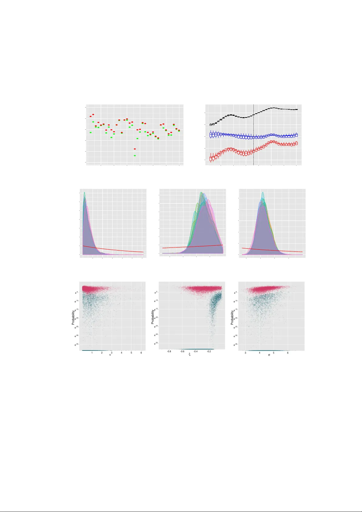
SMC 2 : an efﬁcient algorithm f or sequential analysis of state- space models N. CHOPIN CREST -ENSAE P .E. JA COB CREST & Universit ´ e P aris Dauphine O . P AP ASPILIOPOULOS Universitat P ompeu F abra Summary . W e consider the generic problem of performing sequential Bay esian inference in a state- space model with obser vation process y , state process x and ﬁxed parameter θ . An idealized approach would be to apply the iterated batch impor tance sampling (IBIS) algor ithm of Chopin (2002). This is a sequential Monte Carlo algor ithm in the θ -dimension, that samples values of θ , reweights iteratively these values using the likelihood increments p ( y t | y 1: t − 1 , θ ) , and rejuvenates the θ -par ticles through a resampling step and a MCMC update step . In state-space models these likelihood increments are intractab le in most cases, b ut they ma y be unbiasedly estimated by a par ticle ﬁlter in the x -dimension, f or any ﬁxed θ . This motivates the SMC 2 algorithm proposed in this ar ticle: a sequential Monte Car lo algorithm, deﬁned in the θ -dimension, which propagates and resamples many par ticle ﬁlters in the x -dimension. The ﬁlters in the x -dimension are an example of the random weight par ticle ﬁlter as in F earnhead et al. (2010). On the other hand, the par ticle Markov chain Monte Carlo (PMCMC) frame- work dev eloped in Andrieu et al. (2010) allows us to design appropriate MCMC rejuvenation steps. Thus, the θ -par ticles target the correct posterior distribution at each iteration t , despite the intractabil- ity of the lik elihood increments. W e explore the applicability of our algor ithm in both sequential and non-sequential applications and consider various degrees of freedom, as for example increasing dy- namically the number of x -par ticles. We contrast our approach to various competing methods, both conceptually and empir ically through a detailed simulation study , included here and in a supplement, and based on par ticularly challenging examples. K e ywords : Iter ated batch impor tance sampling; P ar ticle ﬁlter ing; Particle Mar ko v chain Monte Carlo; Sequential Monte Carlo; State-space models 1. Introduction 1.1. Objectives W e consider a generic state-space mo del, with parameters θ ∈ Θ, prior p ( θ ), latent Mark o v pro cess ( x t ), p ( x 1 | θ ) = µ θ ( x 1 ), p ( x t +1 | x 1: t , θ ) = p ( x t +1 | x t , θ ) = f θ ( x t +1 | x t ) , t ≥ 1 , and observ ed pro cess p ( y t | y 1: t − 1 , x 1: t − 1 , θ ) = p ( y t | x t , θ ) = g θ ( y t | x t ) , t ≥ 1 . F or an o v erview of such mo dels with references to a wide range of applications in Engineering, Economics, Natural Sciences, and other ﬁelds, see e.g. Doucet et al. (2001), K ¨ unsc h (2001) or Capp ´ e et al. (2005). W e are interested in the recursive exploration of the sequence of p osterior distributions π 0 ( θ ) = p ( θ ) , π t ( θ , x 1: t ) = p ( θ , x 1: t | y 1: t ) , t ≥ 1 , (1) as well as computing the mo del e vidence p ( y 1: t ) for mo del comp osition. Suc h a sequential analysis of state-space models under parameter uncertain t y is of in terest in many settings; a simple example is out-of-sample prediction, and related go o dness-of-ﬁt diagnostics based on prediction residuals, 2 Chopin et al. whic h are p opular for instance in Econometrics; see e.g. Section 4.3 of Kim et al. (1998) or Ko op and P otter (2007). F urthermore, we shall see that recursiv e exploration up to time t = T may be computationally adv antageous ev en in batch estimation scenarios, where a ﬁxed observ ation record y 1: T is a v ailable. 1.2. State of the ar t Sequen tial Monte Carlo (SMC) methods are considered the state of the art for tackling this kind of problems. Their app eal lies in the eﬃcient re-use of samples across diﬀeren t times t , compared for example with MCMC metho ds which would typically hav e to be re-run for eac h time horizon. Additionally , conv ergence prop erties (with resp ect to the num ber of sim ulations) under mild as- sumptions are no w well understoo d; see e.g. Del Moral and Guionnet (1999), Crisan and Doucet (2002), Chopin (2004), Oudjane and Rub en thaler (2005), Douc and Moulines (2008). See also Del Moral et al. (2006) for a recent ov erview of SMC metho ds. SMC methods are particularly (and rather unarguably) eﬀectiv e for exploring the simpler se- quence of posteriors, π t ( x t | θ ) = p ( x t | y 1: t , θ ); compared to the general case the static parameters are treated as known and in terest is fo cused on x t as opp osed to the whole path x 0: t . This is t ypically called the ﬁltering problem. The corresp onding algorithms are kno wn as p article ﬁlters (PFs); they are describ ed in Section 2.1 in some detail. These algorithms evolv e, weigh t and resample a popu- lation of N x n um b er of particles, x 1: N x t , so that at eac h time t they are a prop erly w eigh ted sample from π t ( x t | θ ). Recall that a particle system is called properly w eigh ted if the weigh ts asso ciated with each sample are unbiased estimates of the Radon-Nikodym deriv ativ e b etw een the target and the prop osal distribution; see for example Section 1 of F earnhead et al. (2010a) and references therein. A by-product of the PF output is an un biased estimator of the likelihoo d incremen ts and the marginal likelihoo d p ( y 1: t | θ ) = p ( y 1 | θ ) t Y s =2 p ( y s | y 1: s − 1 , θ ) , 1 ≤ t ≤ T . (2) the v ariance of which increases linearly ov er time (C ´ erou et al., 2011). Complemen tary to this setting is the iterated batch imp ortance sampling (IBIS) algorithm of Chopin (2002) for the recursive exploration of the sequence of parameter posterior distributions, π t ( θ ); the algorithm is outlined in Section 2.2. This is also an SMC algorithm which updates a p opulation of N θ particles, θ 1: N θ , so that at each time t they are a properly w eigh ted sample from π t ( θ ). The algorithm includes o ccasional MCMC steps for rejuvenating the current p opulation of θ -particles to prev ent the n um b er of distinct θ -particles from decreasing o v er time. Implementation of the algorithm requires the lik elihoo d incremen ts p ( y t | y 1: t − 1 , θ ) to be computable. This constrains the application of IBIS in state-space mo dels since computing the increments inv olv es in tegrating out the latent states. Notable exceptions are linear Gaussian state-space mo dels and mo dels where x t tak es v alues in a ﬁnite set. In such cases a Kalman ﬁlter and a Baum ﬁlter resp ectively can b e associated to each θ -particle to ev aluate eﬃciently the likelihoo d increments; see e.g. Chopin (2007). On the other hand, sequential inference for b oth parameters and laten t states for a generic state-space mo del is a m uc h harder problem, whic h, although very imp ortant in applications, is still rather unresolved; see for example Doucet et al. (2011), Andrieu et al. (2010), Doucet et al. (2009) for re cen t discussions. The batch estimation problem of exploring π T ( θ , x 0: T ) is a non-trivial MCMC problem on its own righ t, esp ecially for large T . This is due to b oth high dep endence b etw een parameters and the latent pro cess, whic h aﬀects Gibbs sampling strategies (P apaspiliop oulos et al., 2007), and the diﬃculty in designing eﬃcient sim ulation schemes for sampling from π T ( x 0: T | θ ). T o address these problems Andrieu et al. (2010) dev elop ed a general theory of particle Mark o v c hain Monte Carlo (PMCMC) algorithms, which are MCMC algorithms that use a particle ﬁlter of size N x as a prop osal mechanism. Sup erﬁcially , it app ears that the algorithm replaces the intractable (2) by the un biased estimator provided by the PF within an MCMC algorithm that samples from π T ( θ ). How ev er, Andrieu et al. (2010) show that (a) as N x gro ws, the PMCMC algorithm behav es more and more lik e the theoretical MCMC algorithm whic h targets the intractable π T ( θ ); and (b) for an y ﬁxed v alue of N x , the PMCMC algorithm admits SMC 2 3 π T ( θ , x 0: T ) as a stationary distribution. The exactness (in terms of not perturbing the stationary distribution) follows from demonstrating that the PMCMC is an ordinary MCMC algorithm (with sp eciﬁc proposal distributions) on an expanded model which includes the PF as auxiliary v ariables; when N x = 1 this augmen tation collapses to the more familiar sc heme of imputing the laten t states. 1.3. Proposed algorithm SMC 2 is a generic blac k b o x tool for p erforming sequen tial analysis of state-space models, which can b e seen as a natural extension of both IBIS and PMCMC. T o each of the N θ θ − particles θ m , we attach a PF which propagates N x x − particles; due to the nested ﬁlters w e call it the SMC 2 algorithm. Unlike the implemen tation of IBIS which carries an exact ﬁlter, in this case the PFs only pro duce unbiased estimates of the marginal likelihoo d. This ensures that the θ - particles are properly weigh ted for π t ( θ ), in the spirit of the r andom weight PF of e.g. F earnhead et al. (2010a). The connection with the auxiliary representation underlying PMCMC is pivotal for designing the MCMC rejuvenation steps, which are crucial for the success of IBIS. W e obtain a sequen tial auxiliary Marko v representation, and use it to formally demonstrate that our algorithm explores the sequence deﬁned in (1). The case N x = ∞ corresp onds to an (unrealisable) IBIS algorithm, whereas N x = 1 to an imp ortance sampling sc heme, the v ariance of which typically gro ws polynomially with t (Chopin, 2004). SMC 2 is a sequential but not an on-line algorithm. The computational load increases with iterations due to the asso ciated cost of the MCMC steps. Nevertheless, these steps typically o ccur at a decreasing rate (see Section 3.8 for details). The only on-line generic algorithm for sequential analysis of state-space mo dels we are aw are of is the self-organizing particle ﬁlter (SOPF) of Kitaga w a (1998): this is PF applied to the extended state ˜ x t = ( x t , θ ), which nev er up dates the θ -comp onen t of particles, and typically div erges quic kly o v er time (e.g. Doucet et al., 2009); see also Liu and W est (2001) for a mo diﬁcation of SOPF which w e discuss later. Th us, a genuinely on-line analysis, which w ould provide constan t Mon te Carlo error at a constant CPU cost, with resp ect to all the comp onents of ( x 1: t , θ ) may well b e an unattainable goal. This is unfortunate, but hardly surprising, given that the target π t is of increasing dimension. F or certain models with a sp eciﬁc structure (e.g the existence of suﬃcien t statistics), an on-line algorithm may b e obtained b y extending SOPF so as to include MCMC up dates of the θ -comp onent, see Gilks and Berzuini (2001), F earnhead (2002), Storvik (2002), and also the more recen t work of Carv alho et al. (2010), but n umerical evidence seems to indicate these algorithms degenerate as well, alb eit p ossibly at a slo w er rate; see e.g. Doucet et al. (2009). On the other hand, SMC 2 is a generic approac h which do es not require such a sp eciﬁc structure. Ev en in batc h estimation scenarios SMC 2 ma y oﬀer sev eral adv an tages o v er PMCMC, in the same wa y that SMC approaches may b e adv an tageous ov er MCMC methods (Neal, 2001; Chopin, 2002; Capp ´ e et al., 2004; Del Moral et al., 2006; Jasra et al., 2007). Under certain conditions (whic h relate to the asymptotic normality of the maximizer of (2)) SMC 2 has the same complexity as PMCMC. Nev ertheless, it calibrates automatically its tuning parameters, as for example N x and the proposal distributions for θ . (Note adaptiv e v ersions of PMCMC, see e.g. Silv a et al. (2009) and Peters et al. (2010) exist how ever.) Then, the ﬁrst iterations of the SMC 2 algorithm make it p ossible to quic kly discard uninteresting parts of the sampling space, using only a small n um b er of observ ations. Finally , the SMC 2 algorithm provides an estimate of the evidence (marginal lik eliho o d) of the mo del p ( y 1: T ) as a direct b y-pro duct. W e demonstrate the p otential of the SMC 2 on tw o classes of problems whic h inv olv e multidi- mensional state pro cesses and several parameters: volatilit y prediction for ﬁnancial assets using L ´ evy driv en sto c hastic v olatilit y mo dels, and lik eliho o d assessmen t of athletic records using time- v arying extreme v alue distributions. A supplemen t to this article (av ailable on the third author’s w eb-page) contains further numerical in v estigations with the SMC 2 and comp eting metho ds on more standard examples. Finally , it has b een p ointed to us that F ulop and Li (2011) ha v e dev elop ed independently and concurren tly an algorithm similar to SMC 2 . Distinctive features of our pap er are the generality of the prop osed approac h, so that it may be used more or less automatically on complex examples (e.g. setting N x dynamically), and the formal results that establish the v alidity of the SMC 2 algorithm, and its complexity . 4 Chopin et al. 1.4. Plan, notations The pap er is organised as follo ws. Section 2 recalls the tw o basic ingredients of SMC 2 : the PF and the IBIS. Section 3 introduces the SMC 2 algorithm, provides its formal justiﬁcation, discusses its complexity and the latitude in its implementation. Section 4 carries out a detailed simulation study which inv estigates the performance of SMC 2 on particularly c hallenging mo dels. Section 5 concludes. As abov e, w e shall use extensively the concise colon notation for sets of random v ariables, e.g. x 1: N x t is a set of N x random v ariables x n t , n = 1 , . . . , N x , x 1: N x 1: t is the union of the sets x 1: N x s , s = 1 , . . . , t , and so on. In the same v ein, 1 : N x stands for the set { 1 , . . . , N x } . P article (resp. time) indices are alw a ys in sup erscript (resp. subscript). The letter p refers to probability densities deﬁned by the model, e.g. p ( θ ), p ( y 1: t | θ ), while π t refers to the probability densit y targeted at time t b y the algorithm, or the corresp onding marginal density with resp ect to its arguments. 2. Preliminaries 2.1. P ar ticle ﬁlters (PFs) W e describ e a particle ﬁlter that approximates recursiv ely the sequence of ﬁltering densities π t ( x t | θ ) = p ( x t | y 1: t , θ ), for a ﬁxed parameter v alue θ . The formalism is chosen with view to in tegrating this algorithm into SMC 2 . W e ﬁrst give a pseudo-co de v ersion, and then we detail the notations. An y op eration inv olving the superscript n must be understoo d as p erformed for n ∈ 1 : N x , where N x is the total num b er of particles. Step 1: At iteration t = 1, (a) Sample x n 1 ∼ q 1 ,θ ( · ). (b) Compute and normalise w eigh ts w 1 ,θ ( x n 1 ) = µ θ ( x n 1 ) g θ ( y 1 | x n 1 ) q 1 ,θ ( x n 1 ) , W n 1 ,θ = w 1 ,θ ( x n 1 ) P N x i =1 w 1 ,θ ( x i 1 ) . Step 2: At iteration t = 2 : T , (a) Sample the index a n t − 1 ∼ M ( W 1: N x t − 1 ,θ ) of the ancestor of particle n . (b) Sample x n t ∼ q t,θ ( ·| x a n t − 1 t − 1 ). (c) Compute and normalise w eigh ts w t,θ ( x a n t − 1 t − 1 , x n t ) = f θ ( x n t | x a n t − 1 t − 1 ) g θ ( y t | x n t ) q t,θ ( x n t | x a n t − 1 t − 1 ) , W n t,θ = w t,θ ( x a n t − 1 t − 1 , x n t ) P N x i =1 w t,θ ( x a i t − 1 t − 1 , x i t ) . In this algorithm, M ( W 1: N x t − 1 ,θ ) stands for the multinomial distribution which assigns probability W n t − 1 ,θ to outcome n ∈ 1 : N x , and ( q t,θ ) t ∈ 1: T stands for a sequence of conditional prop osal distributions which depend on θ . A standard, alb eit sub-optimal, choice is the prior, q 1 ,θ ( x 1 ) = µ θ ( x 1 ), q t,θ ( x t | x t − 1 ) = f θ ( x t | x t − 1 ) for t ≥ 2, whic h leads to the simpliﬁcation w t,θ ( x a n t − 1 t − 1 , x n t ) = g θ ( y t | x n t ). W e note in passing that Step (a) is equiv alen t to multinomial resampling (e.g. Gordon et al., 1993). Other, more eﬃcien t schemes exist (Liu and Chen, 1998; Kitagaw a, 1998; Carp enter et al., 1999), but are not discussed in the paper for the sak e of simplicity . A t iteration t , the following quantit y 1 N x N x X n =1 w t,θ ( x a n t − 1 t − 1 , x n t ) SMC 2 5 is an unbiased estimator of p ( y t | y 1: t − 1 , θ ). More generally , it is a key feature of PFs that ˆ Z t ( θ , x 1: N x 1: t , a 1: N x 1: t − 1 ) =  1 N x  t ( N x X n =1 w 1 ,θ ( x n 1 ) ) t Y s =2 ( N x X n =1 w s,θ ( x a n s − 1 s − 1 , x n s ) ) (3) is also an un biased estimator of p ( y 1: t | θ ); this is not a straightforw ard result, see Proposition 7.4.1 in Del Moral (2004). W e denote by ψ 1 ,θ ( x 1: N x 1 ), for t = 1, and ψ t,θ ( x 1: N x 1: t , a 1: N x 1: t − 1 ) for t ≥ 2, the join t probability density of all the random v ariables generated during the course of the algorithm up to iteration t . Thus, the exp ectation of the random v ariable ˆ Z t ( θ , x 1: N x 1: t , a 1: N x 1: t − 1 ) with resp ect to ψ t,θ is exactly p ( y 1: t | θ ). 2.2. Iterated batch impor tance sampling (IBIS) The IBIS approac h of Chopin (2002) is an SMC algorithm for exploring a sequence of parameter p osterior distributions π t ( θ ) = p ( θ | y 1: t ). All the op erations inv olving the particle index m must b e understo o d as op erations p erformed for all m ∈ 1 : N θ , where N θ is the total num b er of θ -particles. Sample θ m from p ( θ ) and set ω m ← 1. Then, at time t = 1 : T (a) Compute the incremental weigh ts and their w eigh ted av erage u t ( θ m ) = p ( y t | y 1: t − 1 , θ m ) , L t = 1 P N θ m =1 ω m × N θ X m =1 ω m u t ( θ m ) , with the conv en tion p ( y 1 | y 1:0 , θ ) = p ( y 1 | θ ) for t = 1. (b) Up date the imp ortance w eigh ts, ω m ← ω m u t ( θ m ) . (4) (c) If some degeneracy criterion is fulﬁlled, sample ˜ θ m indep enden tly from the mixture distribution 1 P N θ m =1 ω m N θ X m =1 ω m K t ( θ m , · ) . Finally , replace the current w eighted particle system, by the set of new, un w eigh ted particles: ( θ m , ω m ) ← ( ˜ θ m , 1) . Chopin (2004) shows that P N θ m =1 ω m ϕ ( θ m ) P N θ m =1 ω m is a consistent and asymptotically (as N θ → ∞ ) normal estimator of the expectations E [ ϕ ( θ ) | y 1: t ] = Z ϕ ( θ ) p ( θ | y 1: t ) dθ , for all appropriately integrable ϕ . In addition, each L t , computed in Step (a), is a consistent and asymptotically normal estimator of the lik elihoo d p ( y t | y 1: t − 1 ). Step (c) is usually decomposed into a resampling and a mutation step. In the ab o v e algorithm the former is done with the multinomial distribution, where particles are selected with probability prop ortional to ω m . As men tioned in Section 2.1 other resampling schemes ma y b e used instead. The mo v e step is achiev ed through a Marko v kernel K t whic h lea v es p ( θ | y 1: t ) in v ariant. In our examples K t will b e a Metropolis-Hastings kernel. A signiﬁcant adv an tage of IBIS is that the p opulation of θ -particles can be used to learn features of the target distribution, e.g by computing b Σ = 1 P N θ m =1 ω m N θ X m =1 ω m ( θ m − ˆ µ ) ( θ m − ˆ µ ) T , ˆ µ = 1 P N θ m =1 ω m N θ X m =1 ω m θ m . 6 Chopin et al. New particles can be proposed according to a Gaussian random w alk ˜ θ m | θ m ∼ N ( θ m , c b Σ), where c is a tuning constan t for achieving optimal scaling of the Metrop olis-Hastings algorithm, or in- dep enden tly ˜ θ m ∼ N ( ˆ µ, b Σ) as suggested in Chopin (2002). A standard degeneracy criterion is ESS < γ N θ , for γ ∈ (0 , 1), where ESS stands for “eﬀective sample size” and is computed as ESS =  P N θ m =1 ω m  2 P N θ m =1 ( ω m ) 2 . (5) Theory and practical guidance on the use of this criterion are provided in Sections 3.7 and 4 resp ectiv ely . In the context of state-space mo dels IBIS is a theoretical algorithm since the lik eliho o d in- cremen ts p ( y t | y 1: t − 1 , θ ) (used b oth in Step 2, and implicitly in the MCMC kernel) are t ypically in tractable. Nevertheless, coupling IBIS with PFs yields a working algorithm as w e sho w in the follo wing section. 3. Sequential parameter and state estimation: the SMC 2 algorithm SMC 2 is a natural amalgamation of IBIS and PF. W e ﬁrst pro vide the algorithm, w e then demon- strate its v alidity and w e close the section b y considering v arious possibilities in its implemen tation. Again, all the op erations in volving the index m must b e understoo d as operations p erformed for all m ∈ 1 : N θ . Sample θ m from p ( θ ) and set ω m ← 1. Then, at time t = 1 , . . . , T , (a) F or each particle θ m , p erform iteration t of the PF described in Section 2.1: If t = 1, sample indep enden tly x 1: N x ,m 1 from ψ 1 ,θ m , and compute ˆ p ( y 1 | θ m ) = 1 N x N x X n =1 w 1 ,θ ( x n,m 1 ); If t > 1, sample  x 1: N x ,m t , a 1: N x ,m t − 1  from ψ t,θ m conditional on  x 1: N x ,m 1: t − 1 , a 1: N x ,m 1: t − 2  , and com- pute ˆ p ( y t | y 1: t − 1 , θ m ) = 1 N x N x X n =1 w t,θ ( x a n,m t − 1 ,m t − 1 , x n,m t ) . (b) Up date the imp ortance w eigh ts, ω m ← ω m ˆ p ( y t | y 1: t − 1 , θ m ) . (6) (c) If some degeneracy criterion is fulﬁlled, sample  ˜ θ m , ˜ x 1: N x ,m 1: t , ˜ a 1: N x 1: t − 1  indep enden tly from the mixture distribution 1 P N θ m =1 ω m N θ X m =1 ω m K t n θ m , x 1: N x ,m 1: t , a 1: N x ,m 1: t − 1  , · o where K t is a PMCMC k ernel describ ed in Section 3.2. Finally , replace the curren t w eigh ted particle system by the set of new unw eigh ted particles: ( θ m , x 1: N x ,m 1: t , a 1: N x ,m 1: t − 1 , ω m ) ← ( ˜ θ m , ˜ x 1: N x ,m 1: t , ˜ a 1: N x ,m 1: t − 1 , 1) . The degeneracy criterion in Step (c) will t ypically b e the same as for IBIS, i.e., when the ESS drops b elo w a threshold, where the ESS is computed as in (5) and the ω m ’s are now obtained in (6). W e study the stability and the computational cost of the algorithm when applying this criterion in Section 3.7. SMC 2 7 3.1. F ormal justiﬁcation of SMC 2 A prop er formalisation of the successive imp ortance sampling steps p erformed by the SMC 2 algo- rithm requires extending the sampling space, in order to include all the random v ariables generated b y the algorithm. A t time t = 1, the algorithm generates v ariables θ m from the prior p ( θ ), and for each θ m , the algorithm generates v ectors x 1: N x ,m 1 of particles, from ψ 1 ,θ m ( x 1: N x 1 ). Th us, the sampling space is Θ × X N x , and the actual “particles” of the algorithm are N θ indep enden t and identically distributed copies of the random v ariable ( θ , x 1: N x 1 ), with density: p ( θ ) ψ 1 ,θ ( x 1: N x 1 ) = p ( θ ) N x Y n =1 q 1 ,θ ( x n 1 ) . Then, these particles are assigned importance weigh ts corresp onding to the incremen tal w eigh t function ˆ Z 1 ( θ , x 1: N x 1 ) = N − 1 x P N x n =1 w 1 ,θ ( x n 1 ). This means that, at iteration 1, the target distribu- tion of the algorithm should be deﬁned as: π 1 ( θ , x 1: N x 1 ) = p ( θ ) ψ 1 ,θ ( x 1: N x 1 ) × ˆ Z 1 ( θ , x 1: N x 1 ) p ( y 1 ) , where the normalising constant p ( y 1 ) is easily deduced from the prop erty that ˆ Z 1 ( θ , x 1: N x 1 ) is an un biased estimator of p ( y 1 | θ ). T o understand the prop erties of π 1 , simple manipulations suﬃce. Substituting w 1 ,θ ( x n 1 ), ψ 1 ,θ ( x 1: N x 1 ) and ˆ Z 1 ( θ , x 1: N x 1 ) with their resp ective expressions, π 1 ( θ , x 1: N x 1 ) = p ( θ ) p ( y 1 ) N x Y i =1 q 1 ,θ ( x i 1 ) ( 1 N x N x X n =1 µ θ ( x n 1 ) g θ ( y 1 | x n 1 ) q 1 ,θ ( x n 1 ) ) = 1 N x N x X n =1 p ( θ ) p ( y 1 ) µ θ ( x n 1 ) g θ ( y 1 | x n 1 )    N x Y i =1 ,i 6 = n q 1 ,θ ( x i 1 )    and noting that, for the triplet ( θ , x 1 , y 1 ) of random v ariables, p ( θ ) µ θ ( x 1 ) g θ ( y 1 | x 1 ) = p ( θ , x 1 , y 1 ) = p ( y 1 ) p ( θ | y 1 ) p ( x 1 | y 1 , θ ) one ﬁnally gets that: π 1 ( θ , x 1: N x 1 ) = p ( θ | y 1 ) N x N x X n =1 p ( x n 1 | y 1 , θ )    N x Y i =1 ,i 6 = n q 1 ,θ ( x i 1 )    . The following tw o prop erties of π 1 are easily deduced from this expression. First, the marginal distribution of θ is p ( θ | y 1 ). Thus, at iteration 1 the algori thm is properly w eighted for an y N x . Sec- ond, conditional on θ , π 1 assigns to the v ector x 1: N x 1 a mixture distribution whic h with probabilit y 1 / N x , gives to particle n the ﬁltering distribution p ( x 1 | y 1 , θ ), and to all the remaining particles the prop osal distribution q 1 ,θ . The notation reﬂects these properties b y denoting the target distribution of SMC 2 b y π 1 , since it admits the distributions deﬁned in (1) as marginals. By a simple induction, one sees that the target densit y π t at iteration t ≥ 2 should b e deﬁned as: π t ( θ , x 1: N x 1: t , a 1: N x 1: t − 1 ) = p ( θ ) ψ t,θ ( x 1: N x 1: t , a 1: N x 1: t − 1 ) × ˆ Z t ( θ , x 1: N x 1: t , a 1: N x 1: t − 1 ) p ( y 1: t ) (7) where ˆ Z t ( θ , x 1: N x 1: t , a 1: N x 1: t − 1 ) was deﬁned in (3), that is, it should be prop ortional to the sampling densit y of all random v ariables generated so far, times the pro duct of the successive incremen- tal weigh ts. Again, the normalising constant p ( y 1: t ) in (7) is easily deduced from the fact that ˆ Z t ( θ , x 1: N x 1: t , a 1: N x 1: t − 1 ) is an unbiased estimator of p ( y 1: t | θ ). The follo wing Prop osition gives an alter- nativ e expression for π t . 8 Chopin et al. Proposition 1. The pr ob ability density π t may b e written as: π t ( θ , x 1: N x 1: t , a 1: N x 1: t − 1 ) = p ( θ | y 1: t ) × (8) 1 N x N x X n =1 p ( x n 1: t | θ , y 1: t ) N t − 1 x        N x Y i =1 i 6 = h n t (1) q 1 ,θ ( x i 1 )               t Y s =2 N x Y i =1 i 6 = h n t ( s ) W a i s − 1 s − 1 ,θ q s,θ ( x i s | x a i s − 1 s − 1 )        wher e x n 1: t and h n t ar e deterministic functions of x 1: N x 1: t and a 1: N x 1: t − 1 deﬁne d as fol lows: h n t = ( h n t (1) , . . . , h n t ( t )) denote the index history of x n t , that is, h n t ( t ) = n , and h n t ( s ) = a h n t ( s +1) s , r e cur- sively, for s = t − 1 , . . . , 1 , and x n 1: t = ( x n 1: t (1) , . . . , x n 1: t ( t )) denote the state tr aje ctory of p article x n t , i.e. x n 1: t ( s ) = x h n t ( s ) s , for s = 1 , . . . , t . A pro of is given in App endix A. W e use a b old notation to stress out that the quan tities x n 1: t and h n t are quite diﬀeren t from particle arra ys such as e.g. x 1: N x 1: t : x n 1: t and h n t pro vide the complete genealogy of the particle with lab el n at time t , while x 1: N x 1: t simply concatenates the successive particle arra ys x 1: N x t , and contains no such genealogical information. It follo ws immediately from expression (8) that the marginal distribution of π t with resp ect to θ is p ( θ | y 1: t ). Conditional on θ the remaining random v ariables, x 1: N x 1: t and a 1: N x 1: t − 1 , hav e a mix- ture distribution, according to which, with probabilit y 1 / N x the state tra jectory x n 1: t is generated according to p ( x 1: t | θ , y 1: t ), the ancestor v ariables corresponding to this tra jectory , a h n t ( s ) s are uni- formly distributed within 1 : N x , and all the other random v ariables are generated from the particle ﬁlter proposal distribution, ψ t,θ . Therefore, Prop osition 1 establishes a sequence of auxiliary distri- butions π t on increasing dimensions, whose marginals include the p osterior distributions of in terest deﬁned in (1). The SMC 2 algorithm targets this sequence using SMC techniques. 3.2. The MCMC rejuvenation step T o formally describ e this step p erformed at some iteration t , w e must work, as in the previous section, on the extended set of v ariables ( θ , x 1: N x 1: t , a 1: N x 1: t − 1 ). The algorithm is described below; if the prop osed mov e is accepted, the set of v ariables is replaced by the prop osed one, otherwise it is left unc hanged. The algorithm is based on some prop osal kernel T ( θ, d ˜ θ ) in the θ − dimension, whic h admits probability density T ( θ, ˜ θ ). (The prop osal kernel for θ , T ( θ , · ), ma y b e chosen as describ ed in Section 2.2.) (a) Sample ˜ θ from prop osal kern el, ˜ θ ∼ T ( θ, d ˜ θ ). (b) Run a new PF for ˜ θ : sample indep endently ( ˜ x 1: N x 1: t , ˜ a 1: N x 1: t − 1 ) from ψ t, ˜ θ , and compute ˆ Z t ( ˜ θ , ˜ x 1: N x 1: t , ˜ a 1: N x 1: t − 1 ). (c) Accept the mov e with probabilit y 1 ∧ p ( ˜ θ ) ˆ Z t ( ˜ θ , ˜ x 1: N x 1: t , ˜ a 1: N x 1: t − 1 ) T ( ˜ θ , θ ) p ( θ ) ˆ Z t ( θ , x 1: N x 1: t , a 1: N x 1: t − 1 ) T ( θ, ˜ θ ) . It directly follo ws from (7) that this algorithm deﬁnes a standard Hastings-Metrop olis k ernel with proposal distribution q θ ( ˜ θ , ˜ x 1: N x 1: t , ˜ a 1: N x 1: t ) = T ( θ, ˜ θ ) ψ t, ˜ θ ( ˜ x 1: N x 1: t , ˜ a 1: N x 1: t ) and admits as in v ariant distribution the extended distribution π t ( θ , x 1: N x 1: t , a 1: N x 1: t − 1 ). In the broad PMCMC framew ork, this scheme corresponds to the so-called particle Metrop olis-Hastings algo- rithm (see Andrieu et al., 2010). It is worth p ointing out an interesting digression from the PMCMC framew ork. The Marko v mutation k ernel has to b e inv arian t with respect to π t , but it do es not necessarily need to pro duce an ergodic Mark ov chain, since consistency of Monte Carlo estimates is achiev ed by a v eraging across man y particles and not within a path of a single particle. Hence, w e can also attempt low er dimensional up dates, e.g using a Hastings-within-Gibbs algorithm. The adv antage of such mov es is that they migh t lead to higher acceptance rates for the same step size in the θ -dimension. How ev er, we do not pursue this p oint further in this article. SMC 2 9 3.3. PMCMC’ s inv ariant distr ibution, state inf erence F rom (8), one may rewrite π t as the marginal distribution of ( θ, x 1: N x 1: t , a 1: N x 1: t − 1 ) with resp ect to an extended distribution that would include a uniformly distributed particle index n ? ∈ 1 : N x : π ? t ( n ? , θ , x 1: N x 1: t , a 1: N x 1: t − 1 ) = p ( θ | y 1: t ) N t x × p ( x n ? 1: t | θ , y 1: t )        N x Y i =1 i 6 = h n ? t (1) q 1 ,θ ( x i 1 )               t Y s =2 N x Y i =1 i 6 = h n ? t ( s ) W a i s − 1 s − 1 ,θ q s,θ ( x i s | x a i s − 1 s − 1 )        . (9) Andrieu et al. (2010) formalise PMCMC algorithms as MCMC algorithms that leav es π ? t in v ari- an t, whereas in the previous section we justiﬁed our PMCMC up date as a MCMC step leaving π t in v ariant. This distinction is a mere technicalit y in the PMCMC con text, but it becomes imp ortant in the sequential context. SMC 2 is b est understo o d as an algorithm targetting the sequence ( π t ): deﬁning imp ortance sampling steps b etw een successive v ersions of π ? t seems cum b ersome, as the in terpretation of n ? at time t does not carry ov er to iteration t + 1. This distinction also relates to the concept of Rao-Blackw ellised (marginalised) particle ﬁlters (Doucet et al., 2000): since π t is a marginal distribution with resp ect to π ? t , targetting π t rather than π ? t leads to more eﬃcient (in terms of Monte Carlo v ariance) SMC algorithms. The in terplay betw een π t and π ? t is exploited below and in the follo wing sections in order to fully realize the implemen tation potential of SMC 2 . As a ﬁrst example, direct insp ection of (9) rev eals that the conditional distribution of n ? , giv en θ , x 1: N x 1: t and a 1: N x 1: t − 1 , is M ( W 1: N x t,θ ), the multinomial distribution that assigns probabilit y W n t,θ to outcome n , n ∈ 1 : N x . Therefore, w eigh ted samples from p ( θ, x 1: t | y 1: t ) ma y b e obtained at iteration t as follows: (a) F or m = 1 , . . . , N θ , dra w index n ? ( m ) from M ( W 1: N x t,θ m ). (b) Return the weigh ted sample ( ω m , θ m , x n ? ( m ) ,m 1: t ) m ∈ 1: N θ where x n,m 1: t w as deﬁned in Prop osition 1. This temp or arily extende d particle system can b e used in the standard wa y to mak e inferences ab out x t (ﬁltering), y t +1 (prediction) or even x 1: t (smo othing), under parameter uncertaint y . Smo othing requires to store all the state v ariables x 1: N x , 1: N θ 1: t , which is expensive, but ﬁltering and prediction ma y be p erformed while storing only the most recen t state v ariables, x 1: N x , 1: N θ t . W e discuss more thorough y the memory cost of SMC 2 , and explain ho w smoothing ma y still be carried out at certain times, without storing the complete tra jectories, in Section 3.7. The phrase temp or arily extende d in the previous paragraph refers to our discussion on the diﬀerence betw een π t and π ? t . By extending the particles with a n ? comp onen t, one temporarily c hange the target distribution, from π t to π ? t . T o propagate to time t + 1, one must rev ert back to π t , b y simply marginaling out the particle index n ? . W e note ho w ev er that, b efore rev erting to π t , one has the lib erty to apply MCMC up dates with respect to π ? t . F or instance, one may up date the θ − comp onent of eac h particle according to the full conditional distribution of θ with resp ect to to π ? t , that is, p ( θ | x n ? 1: t , y 1: t ). Of course, this p ossibility is interesting mostly for those mo dels suc h that p ( θ | x n ? 1: t , y 1: t ) is tractable. And, again, this op eration ma y be p erformed only if all the state v ariables are av ailable in memory . 3.4. Reusing all the x − par ticles The previous section describ es an algorithm for obtaining a particle sample ( ω m , θ m , x n ? ( m ) ,m 1: t ) m ∈ 1: N θ that targets p ( θ, x 1: t | y 1: t ). One ma y use this sample to compute, for an y test function h ( θ , x 1: t ), an estimator of the exp ectation of h with resp ect to the target p ( θ , x 1: t | y 1: t ): 1 P N θ m =1 ω m N θ X m =1 ω m h ( θ m , x n ? ( m ) ,m 1: t ) . 10 Chopin et al. As in Andrieu et al. (2010, Section 4.6), we ma y deduce from this expression a Rao-Blackw ellised estimator, b y marginalising out n ? , and re-using all the x -particles: 1 P N θ m =1 ω m N θ X m =1 ω m ( N x X n =1 W n t,θ m h ( θ m , x n,m 1: t ) ) . The v ariance reduction obtained b y this Rao-Blackw ellisation scheme should dep end on the v ari- abilit y of h ( θ m , x n,m 1: t ) with resp ect to n . F or a ﬁxed m , the comp onents x n,m 1: t ( s ) of the tra- jectories x n,m 1: t are diverse when s is close to t , and degenerate when s is small. Thus, this Rao-Blac kw ellisation scheme should b e more eﬃcient when h depends mostly on recent state v al- ues, e.g. h ( θ , x 1: t ) = h ( x t ), and less eﬃcien t when h dep ends mostly on early state v alues, e.g. h ( θ , x 1: t ) = h ( x 1 ). 3.5. Evidence The evidence of the data obtained up to time t may b e decomp osed using the c hain rule: p ( y 1: t ) = t Y s =1 p ( y s | y 1: s − 1 ) . The IBIS algorithm delivers the w eigh ted a v erages L s , for each s = 1 , . . . , t , which are Mon te Carlo estimates of the corresp onding factors in the product; see Section 2.2. Thus, it pro vides an estimate of the evidence b y m ultiplying these terms. This can also b e achiev ed via the SMC 2 algorithm in a similar manner: ˆ L t = 1 P N θ m =1 ω m N θ X m =1 ω m ˆ p ( y t | y 1: t − 1 , θ m ) where ˆ p ( y t | y 1: t − 1 , θ m ) is giv en in the deﬁnition of the algorithm. It is therefore p ossible to estimate the evidence of the mo del, at each iteration t , at practically no extra cost. 3.6. A utomatic calibration of N x The plain v anilla SMC 2 algorithm assumes that N x sta ys constan t during the complete run. This p oses tw o practical diﬃculties. First, c ho osing a mo derate v alue of N x that leads to a go o d per- formance (in terms of small Mon te Carlo error) is typically diﬃcult, and may require tedious pilot runs. As an y tuning parameter, it w ould b e nice to design a strategy that determines automatically a reasonable v alue of N x . Second, Andrieu et al. (2010) show that, in order to obtain reasonable acceptance rates for a particle Metrop olis-Hastings step, one should tak e N x = O ( t ), where t is the n um b er of data-points currently considered. In the SMC 2 con text, this means that it may make sense to use a small v alue for N x for the early iterations, and then to increase it regularly . Finally , when the v ariance of the PF estimates dep ends on θ , it might b e in teresting to allow N x to change with θ as w ell. The SMC 2 framew ork pro vides more scope for such adaptation compared to PMCMC. In this section w e describe t wo possibilities, whic h relate to the t wo main particle MCMC methods, particle marginal Metrop olis-Hastings and particle Gibbs. The former generates the auxiliary v ariables indep enden tly of the current particle system whereas the latter do es it conditionally on the current system. F or this reason the latter yields a new system without c hanging the weigh ts, which is a nice feature, but it requires storing particle histories, whic h is memory ineﬃcient; see Section 3.7 for a more thorough discussion of the memory cost of SMC 2 . The sc hemes for increasing N x can b e integrated into the main SMC 2 algorithm along with rules for automatic calibration. W e propose the following simple strategy . W e start with a small v alue for N x , we monitor the acceptance rate of the PMCMC step and when this rate falls b elow a giv en threshold, we trigger the “c hanging N x ” step; for example w e m ultiply N x b y 2. SMC 2 11 3.6.1. Exc hange importance sampling step Our ﬁrst suggestion inv olves a particle exc hange. At iteration t , the algorithm has generated so far the random v ariables θ 1: N θ , x 1: N x , 1: N θ 1: t and a 1: N x , 1: N θ 1: t − 1 and the target distribution is π t ( θ , x 1: N x 1: t , a 1: N x 1: t − 1 ). A t this stage, one may extend the sampling space, by generating for each particle θ m , new PFs of size ˜ N x , b y simply sampling indep enden tly , for eac h m , the random v ariables ˜ x 1: ˜ N x ,m 1: t , ˜ a 1: ˜ N x ,m 1: t − 1 from ψ t,θ m . Th us, the extended target distribution is: π t ( θ , x 1: N x 1: t , a 1: N x 1: t − 1 ) ψ t,θ ( ˜ x 1: ˜ N x 1: t , ˜ a 1: ˜ N x 1: t − 1 ) . (10) In order to sw ap the x − particles and the ˜ x − particles, we use the generalised imp ortance sampling strategy of Del Moral et al. (2006), which is based on an artiﬁcial backw ard kernel. Using (7), we compute the incremental weigh ts π t ( θ , ˜ x 1: ˜ N x 1: t , ˜ a 1: ˜ N x 1: t − 1 ) L t  ( θ , ˜ x 1: ˜ N x 1: t , ˜ a 1: ˜ N x 1: t − 1 ) , ( x 1: N x 1: t , a 1: N x 1: t − 1 )  π t ( θ , x 1: N x 1: t , a 1: N x 1: t − 1 ) ψ t,θ ( ˜ x 1: ˜ N x 1: t , ˜ a 1: ˜ N x 1: t − 1 ) (11) = ˆ Z t ( θ , ˜ x 1: ˜ N x 1: t , ˜ a 1: ˜ N x 1: t − 1 ) ˆ Z t ( θ , x 1: N x 1: t , a 1: N x 1: t − 1 ) × L t  ( θ , ˜ x 1: ˜ N x 1: t , ˜ a 1: ˜ N x 1: t − 1 ) , ( x 1: N x 1: t , a 1: N x 1: t − 1 )  ψ t,θ ( x 1: N x 1: t , a 1: N x 1: t − 1 ) where L t is a bac kward kernel densit y . One then ma y drop the “old” particles ( x 1: N x 1: t , a 1: N x 1: t − 1 ) in order to obtain a new particle system, based on particles ( θ, ˜ x 1: ˜ N x 1: t , ˜ a 1: ˜ N x 1: t − 1 ) targetting π t , but with ˜ N x , x − particles. This importance sampling op eration is v alid under mild assumptions for the bac kw ard kernel L t ; namely that the supp ort of the denominator of (11) is included in the support of its numerator. One easily deduces from Proposition 1 of Del Moral et al. (2006) and (7) that the optimal k ernel (in terms of minimising the v ariance of the weigh ts) is L opt t  ( θ , ˜ x 1: ˜ N x 1: t , ˜ a 1: ˜ N x 1: t − 1 ) , ( x 1: N x 1: t , a 1: N x 1: t − 1 )  = ψ t,θ ( x 1: N x 1: t , a 1: N x 1: t − 1 ) ˆ Z t ( θ , x 1: N x 1: t , a 1: N x 1: t − 1 ) p ( y 1: t | θ ) . This function is intractable, b ecause of the denominator p ( y 1: t | θ ), but it suggests the following simple approximation: L t should b e set to ψ t,θ , so as to cancel the second ratio, which leads to the v ery simple incremental weigh t function: u exch t  θ , x 1: N x 1: t , a 1: N x 1: t − 1 , ˜ x 1: ˜ N x 1: t , ˜ a 1: ˜ N x 1: t − 1  = ˆ Z t ( θ , ˜ x 1: ˜ N x 1: t , ˜ a 1: ˜ N x 1: t − 1 ) ˆ Z t ( θ , x 1: N x 1: t , a 1: N x 1: t − 1 ) . By default, one may implement this exchange step for all the particles θ 1: N θ , and m ultiply consequen tly eac h particle weigh t ω m with the ratio ab ov e. How ev er, it is p ossible to apply this step to only a subset of particles, either selected randomly or according to some deterministic criterion based on θ . (In that case, only the w eights of the selected particles should b e up dated.) Similarly , one could up date certain particles according to a Hastings-Metrop olis step, where the exc hange op eration is prop osed, and accepted with probabilt y the minim um of 1 and the ratio ab o v e. In b oth cases, one eﬀectively targets a mixture of π t distributions corresp onding to diﬀerent v alues of N x . This does not p ose any formal diﬃcutly , b ecause these distributions admit the same marginal distributions with respect to the comp onents of interest ( θ , and x 1: t if the target distri- bution is extended as describ ed in Section 3.3), and b ecause the successiv e importance sampling steps (suc h as either the exchange step ab ov e, or Step (b) in the SMC 2 Algorithm) correspond to ratios of densities that are kno wn up to a constan t that do es not dep end on N x . Of course, in practice, propagating PF of v arying size N x is a bit more cumbersome to imple- men t, but it ma y sho w useful in particular applications, where for instance the computational cost of sampling a new state x t +1 , conditional on x t , v aries strongly according to θ . 12 Chopin et al. 3.6.2. Conditional SMC step Whereas the exc hange steps asso ciates with the target π t , and the particle Metrop olis-Hastings algorithm, our second suggestion relates to the target π ? t , and to the particle Gibbs algorithm. First, one extends the target distribution, from π t to π ? t , by sampling a particle index n ? , as explained in Section 3.3. Then one ma y apply a conditional SMC step (Andrieu et al., 2010), to generate a new particle ﬁlter of size ˜ N x , ˜ x 1: ˜ N x 1: t , ˜ a 1: ˜ N x 1: t − 1 , but conditional on one tra jectory b eing equal to x n 1: t . This amoun ts to sampling the conditional distribution deﬁned b y the tw o factors in curly brac k ets in (9), which can also be conv enien tly rewritten as N t x π ? t ( n ? , θ , ˜ x 1: ˜ N x 1: t , ˜ a 1: ˜ N x 1: t − 1 ) p ( θ , x n 1: t | y 1: t ) . W e refrain from calling this operation a Gibbs step, b ecause it changes the target distribution (and in particular its dimension), from π t ( θ , x 1: N x 1: t , a 1: N x 1: t ) to π t ( θ , x 1: ˜ N x 1: t , a 1: ˜ N x 1: t ). A better formali- sation is again in terms of an imp ortance sampling step in volving a bac kward k ernel (Del Moral et al., 2006), from the proposal distribution, the curren t target distribution π t times the conditional distribution of the newly generated v ariables: π ? t ( n ? , θ , x 1: N x 1: t , a 1: N x 1: t − 1 ) N t x π ? t ( n ? , θ , ˜ x 1: ˜ N x 1: t , ˜ a 1: ˜ N x 1: t − 1 ) p ( θ , x n 1: t | y 1: t ) to w ards target distribution π ? t ( n ? , θ , ˜ x 1: ˜ N x 1: t , ˜ a 1: ˜ N x 1: t − 1 ) L t  ( n ? , θ , ˜ x 1: ˜ N x 1: t , ˜ a 1: ˜ N x 1: t − 1 ) , ·  where L t is again an arbitrary bac kw ard kernel, whose argument, denoted by a dot, is all the v ariables in ( x 1: N x 1: t , a 1: N x 1: t − 1 ), except the v ariables corresp onding to tra jectory x n 1: t . It is easy to see that the optimal bac kw ard kernel (applying again Prop osition 1 of Del Moral et al. 2006) is such that the imp ortance sampling ratio equals one. The main drawbac k of this approac h is that it requires to store all the state v ariables x 1: N x , 1: N θ 1: t ; see our dicussion of memory cost in Section 3.7. 3.7. Comple xity 3.7.1. Memory cost In full generalit y the SMC 2 algorithm is memory-in tensiv e: up to iteration t , O ( tN θ N x ) v ariables ha v e b een generated and p oten tially hav e to b e carried forward to the next iteration. W e explain no w ho w this cost can be reduced to O ( N θ N x ) with little loss of generalit y . Only the v ariables x 1: N x , 1: N θ t − 1 are necessary to carry out Step (a) of the algorithm, while all other state v ariables x 1: N x , 1: N θ 1: t − 2 can b e discarded. Additionally , when Step (c) is carried out as described in Section 3.2, ˆ Z t is the only additional necessary statistic of the particle histories. Thus, the t ypical implementation of SMC 2 for sequential parameter estimation, ﬁltering and prediction has an O ( N θ N x ) memory cost. The memory cost of the exchange step is also O ( N x N θ ); more precisely , it is O ( ˜ N x N θ ), where ˜ N x is the new size of the PF’s. A nice property of this exchange step is that it temp orarily regenerates complete tra jectories x 1: ˜ N x ,m 1: t , sequentially for m = 1 , . . . , M . Thus, b esides augmenting N x dynamically , the exchange step can also b e used to to carry out op erations in v olving complete tra jectories at certain pre-deﬁned times, while maintaining a O ( N θ ˜ N x ) o v erall cost. Such operations include inference with respect to π t ( θ , x 1: t ), up dating θ with resp ect to the full conditional p ( θ | x 1: t , y 1: t ), as explained in Section 3.3, or ev en the conditional SMC up date descrided in Section 3.6.2. 3.7.2. Stabilit y and computational cost Step (c), which requires re-estimating the lik eliho od, is the most computationally expensive comp o- nen t of SMC 2 . When this op eration is p erformed at time t , it incurs an O ( tN θ N x ) computational cost. Therefore, to study the computational cost of SMC 2 w e need to inv estigate the rate at which SMC 2 13 ESS drops b elo w a given threshold. This question directly relates to the stabilit y of the ﬁlter, and w e will work as in Section 3.1 of Chopin (2004) to answer it. Our approac h is based on certain simplifying assumptions, regularit y conditions and a recen t result of C ´ erou et al. (2011) whic h all lead to Prop osition 2; the assumptions are discussed in some detail in App endix B. In general, ESS / N θ < γ , for ESS given in (5), is a standard degeneracy criterion of sequential imp ortance sampling due to the fact that the limit of ESS / N θ as N θ → ∞ is equal to the inv erse of the second momen t of the importance sampling w eights (normalized to ha ve mean 1). This limiting quan tit y , which w e will generically denote b y E , is also often called eﬀective sample size since it can b e in terpreted as an equiv alent n um ber of indep endent samples from the target distribution (see Section 2.5.3 of Liu, 2008, for details). The ﬁrst simpliﬁcation in our analysis is to study the prop erties of E , rather than its ﬁnite sample estimator ESS / N θ , and consider an algorithm which resamples whenev er E < γ . Consider no w the sp eciﬁc context of SMC 2 . Let t b e a resampling time at which equally w eigh ted, indep endent particles hav e b een obtained, and t + p, p > 0, a future time such that no resampling has happ ened since t . The marginal distribution of the resampled particles at time t is only appro ximately π t due to the burn-in perio d of the Marko v chains which are used to generate them. The second simplifying assumption in our analysis is that this marginal distribution is precisely π t . Under this assumption, the particles at time t + p are generated according to the distribution ¯ π t,t + p , ¯ π t,t + p ( θ , x 1: N x 1: t + p , a 1: N x 1: t + p − 1 ) = π t ( θ , x 1: N x 1: t , a 1: N x 1: t − 1 ) ψ t + p,θ ( x 1: N x 1: t + p , a 1: N x 1: t + p − 1 | x 1: N x 1: t , a 1: N x 1: t − 1 ) and the exp ected v alue of the weigh ts ω t + p obtained from (6) is p ( y 1: t ) /p ( y 1: t + p ). Therefore, the normalized w eigh ts are given by p ( y 1: t ) p ( y 1: t + p ) p Y i =1 ˆ p ( y t + i | y 1: t + i − 1 , θ ) ∆ = ˆ Z t + p | t ( θ , x 1: N x 1: t + p , a 1: N x 1: t + p − 1 ) p ( y t +1: t + p | y 1: t ) , and the inv erse of the second momen t of the normalized w eigh ts in SMC 2 and IBIS is given by E N x t,t + p = ( E ¯ π t,t + p " ˆ Z t + p | t ( θ , x 1: N x 1: t + p , a 1: N x 1: t + p − 1 ) 2 p ( y t +1: t + p | y 1: t ) 2 #) − 1 , E ∞ t,t + p =  E p ( θ | y 1: t )  p ( θ | y 1: t + p ) 2 p ( θ | y 1: t ) 2  − 1 . The previous developmen t leads to the follo wing Prop osition which is prov ed in App endix B. Proposition 2. (a) Under Assumptions (H1a) and (H1b) in App endix B, ther e exists a c onstant η > 0 such that for any p , if N x > η p , E N x t,t + p ≥ 1 2 E ∞ t,t + p . (12) (b) Under Assumptions (H2a)-(H2d) in App endix B, for any γ > 0 ther e exist τ , η > 0 and t 0 < ∞ , such that for t ≥ t 0 , E N x t,t + p ≥ γ , for p = d τ t e , N x = d η t e . The implication of this Prop osition is the following: under the assumptions in App endix B and the assumption that the resampling step pro duces samples from the target distribution, the resample steps should b e triggered at times  τ k  , k ≥ 1, to ensure that the weigh t degeneracy b et w een t w o successiv e resampling step stays b ounded in the run of the algorithm; at these times N x should be adjusted to N x =  η τ k  ; th us, the cost of eac h successive imp ortance sampling step is O ( N θ τ k ), until the next resampling step; a simple calculation shows that the cumulativ e compu- tational cost of the algorithm up to some iteration t is then O ( N θ t 2 ). This is to b e contrasted with a computational cost O ( N θ t ) for IBIS under a similar set of assumptions. The assumptions which lead to this result are restrictive but they are typical of the state of the art for obtaining results ab out the stability of this type of sequential algorithms; see App endix B for further discussion. 14 Chopin et al. 4. Numerical illustrations An initial study whic h illustrates SMC 2 in a range of examples of moderate diﬃculty is av ailable from the second author’s web-page, see http://sites.google.com/site/pierrejacob/, as supplemen- tary material. In that study , SMC 2 w as shown to typically outp erform comp eting algorithms, whether in sequential scenarios (where datapoints are obtained sequentially) or in batch scenarios (where the only distribution of in terest is p ( θ , x 1: T | y 1: T ) for some ﬁxed time horizon T ). F or in- stance, in the former case, SMC 2 w as shown to provide smaller Monte Carlo errors than the SOPF at a given CPU cost. In the latter case, SMC 2 w as sho wn to compare fav ourably to an adaptiv e v ersion of the marginal PMCMC algorithm prop osed by Peters et al. (2010). In this pap er, our ob jective instead is to tak e a hammer to SMC 2 , that is, to ev aluate its p erformance on mo dels that are regarded as particularly challenging, ev en for batch estimation purp oses. In addition, we treat SMC 2 as muc h as p ossible as a black b ox: the num b er N x of x -particles is augmented dynamically (using the exchange step, see Section 3.6.1), as explained in Section 3.6; the mov e steps are calibrated using the curren t particles, as describ ed at the end of Section 2.2, and so on. The only model-dep endent inputs are (a) a procedure for sampling from the Mark o v transition of the mo del, f θ ( x t +1 | x t ); (b) a procedure for p oint wise ev aluation the lik eliho o d g θ ( y t | x t ); and (c) a prior distribution on the parameters. This means that the prop osal q t,θ is set to the default choice f θ ( x t +1 | x t ). This also means that w e are able to treat mo dels such that the densit y f θ ( x t +1 | x t ) cannot b e computed, even if it ma y be sampled from; this is the case in the ﬁrst application we consider. A generic SMC 2 soft w are pac k age written in Python and C b y the second author is av ailable at h ttp://code.go ogle.com/p/py-smc2/. 4.1. Sequential prediction of asset price volatility SMC 2 is particularly well suited to tac kle sev eral of the c hallenges that arise in the probabilistic mo delling of ﬁnancial time series: prediction is of central importance; risk management requires accoun ting for parameter and model uncertain t y; non-linear models are necessary to capture the features in the data; the length of t ypical time series is large when mo delling medium/low frequency data and v ast when considering high frequency observ ations. W e illustrate some of these possibilities in the con text of prediction of daily volatilit y of asset prices. There is a v ast literature on sto chastic volatilit y (SV) mo dels; w e simply refer to the excellen t exp osition in Barndorﬀ-Nielsen and Shephard (2002) for references, persp ectives and second-order prop erties. The generic framework for daily volatilit y is as follows. Let s t b e the v alue of a giv en ﬁnancial asset (e.g a stock price or an exchange rate) on the t -th da y , and y t = 10 5 / 2 log( s t /s t − 1 ) b e the so-called log-returns (the scaling is done for n umerical conv enience). The SV model sp eciﬁes a state-space mo del with observ ation equation: y t = µ + β v t + v 1 / 2 t  t , t ≥ 1 (13) where the  t is a sequence of independent errors which are assumed to b e standard Gaussian. The pro cess v t is kno wn as the actual v olatilit y and it is treated as a stationary stochastic process. This implies that log-returns are stationary with mixed Gaussian marginal distribution. The co eﬃcient β has b oth a ﬁnancial interpretation, as a risk premium for excess volatilit y , and a statistical one, since for β 6 = 0 the marginal density of log-returns is sk ew ed. W e consider the class of L ´ evy driven SV mo dels whic h were in troduced in Barndorﬀ-Nielsen and Shephard (2001) and hav e been intensiv ely studied in the last decade from both the mathematical ﬁnance and the statistical communit y . This family of mo dels is speciﬁed via a contin uous-time mo del for the joint ev olution of log-price and sp ot (instan taneous) v olatilit y , whic h are driven by Bro wnian motion and L ´ evy process resp ectively . The actual volatilit y is the integral of the sp ot v olatilit y o v er daily interv als, and the contin uous-time mo del translates in to a state-space model for y t and v t as w e show b elow. Details can b e found in Sections 2 (for the con tin uous-time sp eciﬁcation) and 5 (for the state-space representation) of the original article. Likelihoo d-based inference for this class of mo dels is recognized as a very c hallenging problem, and it has b een undertak en among others in Rob erts et al. (2004); Griﬃn and Steel (2006) and most recently in Andrieu et al. (2010) using PMCMC. On the other hand, Barndorﬀ-Nielsen and Shephard (2002) SMC 2 15 dev elop quasi-likelihoo d metho ds using the Kalman ﬁlter based on an approximate state-space form ulation suggested by the second-order prop erties of the ( y t , v t ) process. Here we fo cus on mo dels where the bac kground driving L ´ evy pro cess is expressed in terms of a ﬁnite rate Poisson pro cess and consider m ulti-factor speciﬁcations of such mo dels which include lev erage. This c hoice allo ws the exact sim ulation of the actual v olatility process, and permits direct comparisons to the n umerical results in Sections 4 of Rob erts et al. (2004), 3.2 of Barndorﬀ-Nielsen and Shephard (2002) and 6 of Griﬃn and Steel (2006). Additionally , this case is representativ e of a system whic h can b e very easily simulated forwards whereas computation of its transition densit y is considerably in v olv ed (see (14) b elow). The speciﬁcation for the one-factor mo del is as follo ws. W e parametrize the laten t process as in Barndorﬀ-Nielsen and Shephard (2002) in terms of ( ξ , ω 2 , λ ) where ξ and ω 2 are the stationary mean and v ariance of the sp ot volatilit y process, and λ the exponential rate of decay of its auto correlation function. The second-order prop erties of v t can be expressed as functions of these parameters, see Section 2.2 of Barndorﬀ-Nielsen and Shephard (2002). The state dynamics for the actual volatilit y are as follo ws: k ∼ Poi  λξ 2 /ω 2  , c 1: k iid ∼ U( t, t + 1) , e 1: k iid ∼ Exp  ξ /ω 2  , z t +1 = e − λ z t + k X j =1 e − λ ( t +1 − c j ) e j , v t +1 = 1 λ   z t − z t +1 + k X j =1 e j   , x t +1 = ( v t +1 , z t +1 ) 0 . (14) In this representation, z t is the discretely-sampled sp ot volatilit y pro cess, and the Marko vian represen tation of the state pro cess inv olv es the pair ( v t , z t ). The random v ariables ( k , c 1: k , e 1: k ) are generated indep endently for each time p erio d, and 1 : k is understoo d as the empt y set when k = 0. These system dynamics imply a Γ( ξ 2 /ω 2 , ξ /ω 2 ) as stationary distribution for z t . Therefore, w e tak e this to b e the initial distribution for z 0 . W e applied the algorithm to a synthetic data set of length T = 1 , 000 (Figure 1(a)) simulated with the v alues µ = 0, β = 0, ξ = 0 . 5, ω 2 = 0 . 0625, λ = 0 . 01 which were used also in the sim ulation study of Barndorﬀ-Nielsen and Shephard (2002). W e launched 5 indep enden t runs using N θ = 1 , 000, a ESS threshold set at 50%, and the independent Hastings-Metrop olis scheme describ ed in Section 2.2. The n um b er N x w as set initially to 100, and increased whenever the acceptance rate w en t b elo w 20% (Figure 1(b)-(c)). Figure 1(d)-(e) shows estimates of the posterior marginal distribution of some parameters. Note the impact the large jump in the v olatilit y has on N x , which is systematically (across runs) increased around time 400, and the p osterior distribution of the parameters of the v olatilit y pro cess, see Figure 1(f ). It is interesting to compare the numerical p erformance of SMC 2 to that of the SOPF and Liu and W est (2001)’s particle ﬁlter (referred to as L&W in the following) for this model and data, and for a comparable CPU budget. The SOPF, if run with N = 10 5 particles, collapses to one single particle at ab out t = 700 and is thus completely un usable in this context. L&W is a version of SOPF where the θ -comp onents of the particles are div ersiﬁed using a Gaussian mov e that lea ves the ﬁrst t w o empirical momen ts of the particle sample unc hanged. This mov e unfortunately introduces a bias which is hard to quan tity . W e implemented L&W with N = 2 × 10 5 ( x, θ )-particles and w e set the smo othing parameter h to 10 − 1 ; see the Supplemen t for results with v arious v alues of h . This num b er of particles w as to chosen to make the computing time of SMC 2 and L&W comparable, see Figure 2(a). Unsurprisingly , L&W runs are very consisten t in terms of computing times, whereas those of SMC 2 are more v ariable, mainly b ecause the n umber of x -particles does not reach the same v alue across the runs and the n umber of resample-mov e steps v aries. Each of these runs to ok b etw een 1 . 5 and 7 hours using a simple Python script and only one pro cessing unit of a 2008 desktop computer (equipp ed with an Intel Core 2 Duo E8400). Note that, given that these metho ds could easily b e parallelized, the computational cost can b e greatly reduced; a 100 × sp eed-up is plausible using appropriate hardw are. Our results suggest that the bias in L&W is signiﬁcant. Figure 2(b) shows the p osterior distribution of ξ , the mean of v olatilit y , at time t = 500, which is about 100 time steps after the large jump in volatilit y at time t = 407. The results for both algorithms are compared to those from a long PMCMC run (implemented as in Peters et al., 2010, and detailed in the Supplement) with N x = 500 and 10 5 iterations. Figure 2(c) reports on the estimation of the log evidence log p ( y 1: t ) 16 Chopin et al. Time Squared observations 0 2 4 6 8 200 400 600 800 1000 (a) Time Acceptance rates 0.0 0.2 0.4 0.6 0.8 1.0 ● ● ● ● ● ● ● ● ● ● ● ● ● ● ● ● ● ● ● ● ● ● ● ● ● ● ● ● ● ● ● ● ● ● ● ● ● ● ● ● ● ● ● ● ● ● ● ● ● ● ● ● ● ● ● ● ● ● ● ● ● ● ● ● ● ● ● ● ● ● ● ● ● ● ● ● ● ● ● ● ● ● ● ● ● ● ● ● ● ● ● ● ● ● ● ● ● ● ● ● ● ● ● ● ● ● ● ● ● ● ● ● ● ● ● ● ● ● ● ● ● ● ● ● ● ● ● ● ● ● ● ● ● ● ● ● ● ● ● ● ● ● ● ● ● ● ● ● ● ● ● ● ● ● ● ● ● ● ● 0 200 400 600 800 1000 run ● 1 ● 2 ● 3 ● 4 ● 5 (b) Time N x 500 1000 1500 2000 2500 3000 ● ● ● ● ● ● ● ● ● ● ● ● ● ● ● ● ● ● ● ● ● ● ● ● ● ● ● ● ● ● ● 0 200 400 600 800 1000 run ● 1 ● 2 ● 3 ● 4 ● 5 (c) µ density 0 1 2 3 4 5 6 7 250 −0.5 0.0 0.5 1.0 500 −0.5 0.0 0.5 1.0 1000 −0.5 0.0 0.5 1.0 Run 1 2 3 4 5 (d) β density 0.0 0.5 1.0 1.5 2.0 2.5 3.0 250 −1.5 −1.0 −0.5 0.0 0.5 1.0 500 −1.5 −1.0 −0.5 0.0 0.5 1.0 1000 −1.5 −1.0 −0.5 0.0 0.5 1.0 Run 1 2 3 4 5 (e) ξ density 0 1 2 3 4 5 250 1 2 3 4 5 6 500 1 2 3 4 5 6 1000 1 2 3 4 5 6 Run 1 2 3 4 5 (f ) Fig. 1. Single-factor stochastic volatility model, synthetic dataset. (a) Squared obser vations vs time. (b)-(f) Results obtained from 5 repeated runs: (b) acceptance rate; (c) N x vs time; (d) to (f) ov erlaid kernel density estimators of the posterior distr ibution of µ , β , ξ at different times t = 250 , 500 , 1000 , the vertical dashed line indicates the true value and solid red lines the prior density . SMC 2 17 for each algorithm, plotting the estimated log evidence of eac h run minus the mean of the log evidence of the 5 SMC 2 runs. W e see that the log evidence estimated using L&W is systematically biased, positively or negatively dep ending on the time steps, with a large discontin uity at time t = 407, whic h is due to underestimation of the tails of the predictive distribution. Time Computing time (s) 5000 10000 15000 20000 25000 L&W 200 400 600 800 1000 SMC2 200 400 600 800 1000 Run 1 2 3 4 5 (a) ξ density 0.0 0.5 1.0 1.5 2.0 2.5 3.0 3.5 L&W 2 4 6 8 SMC2 2 4 6 8 PMCMC 2 4 6 8 Run 1 2 3 4 5 (b) Time log evidence min us reference −2 −1 0 1 2 L&W 200 400 600 800 SMC2 200 400 600 800 Run 1 2 3 4 5 (c) Fig. 2. Single-f actor stochastic volatility model, synthetic dataset, compar ison between methods. (a) Computing time of 5 independent runs of L&W (left) and SMC 2 (right) in seconds, against time. (b) Estimation of the posterior marginal distr ibution of mean volatility , ξ . (c) Estimation of the log evidence , the curves represent the estimated evidence of each run minus the mean across 5 r uns of the log evidence estimated using SMC 2 . W e now consider mo dels of diﬀerent complexit y for the S&P 500 index. The data set is made of 753 observ ations from January 3rd 2005 to December 31st 2007 and it is shown on Figure 3(a). W e ﬁrst consider a tw o-factor mo del, according to which the actual volatilit y is a sum of tw o inde- p enden t comp onents eac h of whic h follows a L ´ evy driv en mo del. Previous research indicates that a t w o-factor mo del is suﬃciently ﬂexible, whereas more factors do not add signiﬁcantly when consid- ering daily data, see for example Barndorﬀ-Nielsen and Shephard (2002); Griﬃn and Steel (2006) for L ´ evy driven mo dels and Chernov et al. (2003) for diﬀusion-driven SV mo dels. W e consider one comp onen t whic h describes long-term mov ements in the v olatility , with memory parameter λ 1 , and another whic h captures short-term v ariation, with parameter λ 2 >> λ 1 . The second component allo ws more freedom in mo delling the tails of the distribution of log-returns. The contribution of 18 Chopin et al. Time Squared observations 5 10 15 20 100 200 300 400 500 600 700 (a) Time Acceptance rates 0.0 0.2 0.4 0.6 0.8 1.0 ● ● ● ● ● ● ● ● ● ● ● ● ● ● ● ● ● ● ● ● ● ● ● ● ● ● ● ● ● ● ● ● ● ● ● ● ● ● ● ● ● ● ● ● ● ● ● ● ● ● ● ● ● ● ● ● ● ● ● ● ● ● ● ● ● ● ● ● ● ● ● ● ● ● ● ● ● ● ● ● ● ● ● ● 0 100 200 300 400 500 600 700 run ● 1 ● 2 ● 3 (b) Time Log evidence comparison −2 0 2 4 100 200 300 400 500 600 700 Model: Multifactor without le verage Multifactor with le verage (c) Fig. 3. (a): the squares of the S&P 500 data from 03/01/2005 to 21/12/2007. (b): acceptance rates of the resample-mov e step for the full model ov er two independent r uns. (c): log-evidence comparison between models (relative to the one-f actor model). the slo wly mixing process to the o v erall mean and v ariance of the spot volatilit y is con trolled b y the parameter w ∈ (0 , 1). Thus, for this model x t = ( v 1 ,t , z 1 ,t , v 2 ,t , z 2 ,t ) with v t = v 1 ,t + v 2 ,t , where eac h pair ( v i,t , z i,t ) evolv es according to (14) with parameters ( w i ξ , w i ω 2 , λ i ) with w 1 = w , w 2 = 1 − w . The system errors are generated by indep enden t sets of v ariables ( k i , c i, 1: k , e i, 1: k ), and z 0 ,i are initialized according to the corresp onding gamma distributions. Finally , we extend the observ a- tion equation to capture a signiﬁcant feature observed in returns on stocks: low returns prov ok e increase in subsequen t v olatilit y , see for example Black (1976) for an early reference. In parameter driv en SV mo dels, one generic strategy to incorp orate such feedbac k is to correlate the noise in the observ ation and state pro cesses, see Harvey and Shephard (1996) in the context of the logarithmic SV model, and Section 3 of Barndorﬀ-Nielsen and Shephard (2001) for L ´ evy driv en mo dels. W e tak e up their suggestion, and re-write the observ ation equation as y t = µ + β v t + v 1 / 2 t  t + ρ 1 k 1 X j =1 e 1 ,j + ρ 2 k 2 X j =1 e 2 ,j − ξ ( w ρ 1 λ 1 + (1 − w ) ρ 2 λ 2 ) (15) where e i,j are the system error v ariables inv olv ed in the generation of v t and ρ i are the lev erage parameters which we exp ect to b e negative. Thus, in this sp eciﬁcation w e deal with a mo del with a 5-dimensional state and 9 parameters. The mathematical tractabilit y of this family of mo dels and the sp eciﬁcation in terms of station- ary and memory parameters allows to a certain exten t sub jective Ba y esian mo delling. Nev ertheless, since the main emphasis here is to ev aluate the p erformance of SMC 2 w e c ho ose priors that (as we v erify a p osteriori) are rather ﬂat in the areas of high p osterior densit y . Note that the prior for ξ and ω 2 has to reﬂect the scaling of the log-returns by a multiplicativ e factor. W e take an Exp(1) prior for λ 1 , an Exp(0 . 5) for λ 2 − λ 1 , th us imp osing the identiﬁabilit y constraint λ 2 > λ 1 . W e tak e a U(0 , 1) prior for w , an Exp(1 / 5) for ξ and ω 2 , and Gaussian priors with large v ariances for the observ ation equation parameters. W e launc h the three mo dels for the S&P 500 data: single factor, multifactor without and with lev erage; note that multifactor without leverage means the full mo del, but with ρ 1 = ρ 2 = 0 in (15). W e use N θ = 2000, and N x is set initially to 100 and then dynamically increases as already describ ed. The acceptance rates sta y reasonable as illustrated on Figure 3(b). Figure 3(c) sho ws the log evidence log p ( y 1: t ) for the t w o factor mo dels min us the log evidence for the single factor mo del. Negative v alues at time t means that the observ ations fa v our the single factor mo del up to time t . Notice how the mo del evidence changes after the big jump in v olatilit y around time t = 550. Estimated p osterior densities for all parameters are provided in the Supplemen t. 4.2. Assessing e xtreme athletic records The second application illustrates the p otential of SMC 2 in smo othing while accounting for pa- rameter uncertaint y . In particular, we consider state-space mo dels that hav e b een prop osed for SMC 2 19 the dynamic evolution of athletic records, see for example Robinson and T a wn (1995), Gaetan and Grigoletto (2004), F earnhead et al. (2010b). W e analyse the time series of the b est times recorded for w omen’s 3000 metres running even ts b etw een 1976 and 2010. The motiv ation is to assess to whic h exten t W ang Junxia’s w orld record in 1993 w as un usual: 486 . 11 seconds while the previous record was 502 . 62 seconds. The data is sho wn in Figure 4(a) and include tw o observ ations p er year y = y 1:2 , with y 1 < y 2 : y 1 is the b est ann ual time and y 2 the second b est time on the race where y 1 w as recorded. The data is av ailable from http://www.alltime-athletics.com/ and it is further discussed in the aforemen tioned articles. A further fact that sheds doubt on the record is that the second time for 1993 corresp onds to an athlete from the same team as the record holder. W e use the same mo delling as F earnhead et al. (2010b). The observ ations follo w a generalized extreme v alue (GEV) distribution for minima, with cumulativ e distribution function G deﬁned by: G ( y | µ, ξ , σ ) = 1 − exp " −  1 − ξ  y − µ σ  − 1 /ξ + # (16) where µ , ξ and σ are respectively the lo cation, shap e and scale parameters, and {·} + = max(0 , · ). W e denote by g the asso ciated probability densit y function. The supp ort of this distribution dep ends on the parameters; e.g. if ξ < 0, g and G are non-zero for y > µ + σ /ξ . The probabilit y densit y function for y = y 1:2 is giv en by: g ( y 1:2 | µ, ξ , σ ) = { 1 − G ( y 2 | µ, ξ , σ ) } 2 Y i =1 g ( y i | µ, ξ , σ ) 1 − G ( y i | µ, ξ , σ ) (17) sub ject to y 1 < y 2 . The lo cation µ is not treated as a parameter but as a smo oth second-order random w alk pro cess: x t = ( µ t , ˙ µ t ) 0 , x t +1 | x t , ν ∼ N ( F x t , Q ) , F =  1 1 0 1  and Q = ν 2  1 / 3 1 / 2 1 / 2 1  (18) T o complete the model speciﬁcation w e set a diﬀuse initial distribution N (520 , 10 2 ) on µ 0 . Th us w e deal with biv ariate observ ations in time y t = y t, 1:2 , a state-space mo del with non-Gaussian observ ation density given in (17), a tw o-dimensional state pro cess giv en in (18), and a 3-dimensional unkno wn parameter v ector, θ = ( ν, ξ , σ ). W e c ho ose independent exponential prior distributions on ν and σ with rate 0 . 2. The sign of ξ has determining impact on the supp ort of the observ ation densit y , and the computation of extremal probabilities. F or this application, given the form of (16) and the fact that the observ ations are necessarily b ounded from b elow, it makes sense to assume that ξ ≤ 0, hence w e take an exp onential prior distribution on − ξ with rate 0 . 5. (W e also tried a N (0 , 3 2 ) prior, which had some mo derate impact on the estimates presented b elow, but the corresp onding results are not rep orted here.) The data we will use in the analysis exclude the tw o times recorded on 1993. Thus, in an abuse of notation y 1976:2010 b elo w refers to the pairs of times for all y ears but 1993, and in the mo del we assume that there was no observ ation for that year. F ormally w e w an t to estimate probabilities p y t = P ( y t ≤ y | y 1976:2010 ) = Z Θ Z X G ( y | µ t , θ ) p ( µ t | y 1976:2010 , θ ) p ( θ | y 1976:2010 ) dµ t dθ where the smoothing distribution p ( µ t | y 1976:2010 , θ ) and the p osterior distribution p ( θ | y 1976:2010 ) app ear explicitly; b elow we also consider the probabilities conditionally on the parameter v alues, rather than integrating ov er those. The interest lies in p 486 . 11 1993 , p 502 . 62 1993 and p cond t := p 486 . 11 t /p 502 . 62 t , whic h is the probabilit y of observing at year t W ang Junxia’s record given that we observ e a b etter time than the previous world record. The rationale for using this conditional probability is to take in to accoun t the exceptional nature of any new world record. The algorithm is launched 10 times with N θ = 1 , 000 and N x = 250. The resample-mov e steps are triggered when the ESS goes b elow 50%, as in the previous example, and the prop osal distribution used in the mov e steps is an indep endent Gaussian distribution ﬁtted on the particles. The computing time of each of the 10 runs v aries b etw een 30 and 70 seconds (using the same mac hine as in the previous section), which is why we allo w ed ourselves to use a fairly large n um b er 20 Chopin et al. of particles compared to the small time horizon. Figure 4(b) represen ts the estimates ˆ p y t at eac h y ear, for y = 486 . 11 (low er b ox-plots) and y = 502 . 62 (upp er b ox-plots), as well as ˆ p cond t = ˆ p 486 . 11 t / ˆ p 502 . 62 t (middle b ox-plots). The b o x-plots show the v ariability across the indep endent runs of the algorithm, and the lines connect the mean v alues computed across indep enden t runs at eac h y ear. The mean v alue of ˆ p cond 1993 o v er the runs is 9 . 4 · 10 − 4 and the standard deviation ov er the runs is 3 . 3 · 10 − 4 . Note that the estimates ˆ p y t are computed using the smo othing algorithm describ ed in Section 3.3. The second ro w of Figure 4 sho ws the posterior distributions of the three parameters ( ν, ξ , σ ) using k ernel density estimations of the w eighted θ -particles. The densit y estimators obtained for eac h run are o v erlaid to show the consistency of the results ov er indep endent runs. The prior densit y function (full line) is nearly ﬂat ov er the region of high p osterior mass. The third row of Figure 4 shows scatter plots of the probabilities G ( y | µ n ? ( m ) 1993 , θ m ) against the parameters θ m . The triangles represen t these probabilities for y = 486 . 11 while the circles represent the probabilities for y = 502 . 62. The cloud of p oints at the b ottom of these plots corresp ond to parameters θ m for whic h the probability G (486 . 11 | µ n ? ( m ) 1993 , θ m ) is exactly 0. 5. Extensions In this pap er, we developed an “exact approximation” of the IBIS algorithm, that is, an ideal SMC algorithm targetting the sequence π t ( θ ) = p ( θ | y 1: t ), with incremental w eigh t π t ( θ ) /π t − 1 ( θ ) = p ( y t | y 1: t − 1 , θ ). The phrase “exact appro ximation”, borrow ed from Andrieu et al. (2010), refers to the fact that our approac h targets the exact marginal distributions, for any ﬁxed v alue N x . 5.1. Intractab le densities W e ha v e argued that SMC 2 can cop e with state-space mo dels with in tractable transition densities pro vided these can b e simulated from. More generally , it can cop e with in tractable transition of observ ation densities pro vided they can be unbiasedly estimated. Filtering for dynamic models with in tractable densities for which unbiased estimators can be computed w as discussed in F earnhead et al. (2008). It was shown that replacing these densities by their unbiased estimators is equiv alen t to in troducing additional auxiliary v ariables in the state-space mo del. SMC 2 can directly b e applied in this context by replacing these terms by the unbiased estimators to obtain sequential state and parameter inference for such mo dels. 5.2. SMC 2 f or tempering A natural question is whether w e can construct other types of SMC 2 algorithms, which would b e “exact approximations” of diﬀerent SMC strategies. Consider for instance, again for a state-space mo del, the follo wing geometric bridge sequence (in the spirit of e.g. Neal, 2001), which allo ws for a smooth transition from the prior to the posterior: π t ( θ ) ∝ p ( θ ) { p ( y 1: T | θ ) } γ t , γ t = t/L, where L is the total num b er of iterations. As pointed out by one referee, see also F ulop and Duan (2011), it is p ossible to deriv e some sort of SMC 2 algorithm that targets iteratively the sequence π t ( θ ) ∝ p ( θ ) { ˆ p ( y 1: T | θ ) } γ t , γ t = t/L, where ˆ p ( y 1: T | θ ) is a particle ﬁltering estimate of the likelihoo d. Note that { ˆ p ( y 1: T | θ ) } γ t is not an un biased estimate of { p ( y 1: T | θ ) } γ t when γ t ∈ (0 , 1). This mak es the interpretation of the algorithm more diﬃcult, as it cannot b e analysed as a noisy , un biased, version of an ideal algorithm. In particular, Prop osition 2 on the complexit y of SMC 2 cannot b e easily extended to the tempering case. It is also less ﬂexible in terms of PMCMC steps: for instance, it is not p ossible to implement the conditional SMC step described in Section 3.6.2, or more generally a particle Gibbs step, b ecause such steps rely on the mixture representation of the target distribution, where the mixture index is some selected tra jectory , see (9), and this representation do es not hold in the temp ering SMC 2 21 Y ear Times (seconds) 480 490 500 510 520 530 1980 1985 1990 1995 2000 2005 2010 (a) Y ear Probability 10 −5 10 −4 10 −3 10 −2 10 −1 ● ● ● 1980 1985 1990 1995 2000 2005 2010 (b) ν Density 0.0 0.2 0.4 0.6 0.8 1.0 1.2 1.4 1 2 3 4 5 6 (c) ξ Density 0.0 0.5 1.0 1.5 2.0 2.5 3.0 3.5 −0.8 −0.6 −0.4 −0.2 (d) σ Density 0.0 0.2 0.4 0.6 0.8 1.0 3 4 5 6 (e) (f ) (g) (h) Fig. 4. Athletics records. (a) Best tw o times of each year , in women’ s 3000 metres ev ents between 1976 and 2010; (b) box-plots ov er 10 runs of SMC 2 of estimates of the probability of interest (top) p 502 . 62 t , (middle) p cond t and (bottom) p 486 . 11 t ; the y -axis is in log scale and the dotted line indicates the year 1993; (c)-(e) posterior distribution of the parameters approximated by SMC 2 , with results of 10 independent runs overlaid on each plot and where the full line represents the prior density function; (f)-(h) probability of observing at year 1993 a recorded time less than 486 . 11 seconds (blue triangles, low er cloud of points) and less than 502 . 62 seconds (red circles, upper cloud of points) against the components of θ , where point sizes and transparencies are propor tional to the weights of the θ -par ticles. 22 Chopin et al. case. More imp ortan tly , this temp ering strategy do es not mak e it p ossible to p erform sequential analysis as the SMC 2 algorithm discussed in this pap er. The fact remains that this temp ering strategy ma y prov e useful in certain non-sequen tial sce- narios, as suggested by the numerical examples of F ulop and Duan (2011). It may b e used also for determining MAP (maxim um a p osteriori) estimators, and in particular the maxim um likelihoo d estimator (using a ﬂat prior), b y letting γ t → + ∞ . Ackno wledgements N. Chopin is supp orted b y the ANR gran t ANR-008-BLAN-0218 “BigMC” of the F rench Ministry of researc h. P .E. Jacob is supported by a PhD fellowship from the AXA Research F und. O. Pa- paspiliop oulos would like to ac knowledge ﬁnancial supp ort by the Spanish gov ernmen t through a “Ramon y Ca jal” fellowship and grant MTM2009-09063. The authors are thankful to Arnaud Doucet (Univ ersit y of Oxford), P eter M¨ uller (UT Austin), Gareth W. P eters (UCL) and the referees for useful comments. References Andrieu, C., Doucet, A., and Holenstein, R. (2010). Particle Marko v c hain Monte Carlo metho ds. J. R. Statist. So c. B , 72(3):269–342. Andrieu, C. and Rob erts, G. (2009). The pseudo-marginal approac h for eﬃcient Mon te Carlo computations. The Annals of Statistics , 37(2):697–725. Barndorﬀ-Nielsen, O. E. and Shephard, N. (2001). Non-Gaussian Ornstein-Uhlen b ec k-based models and some of their uses in ﬁnancial economics. J. R. Stat. So c. Ser. B Stat. Metho dol. , 63(2):167– 241. Barndorﬀ-Nielsen, O. E. and Shephard, N. (2002). Econometric analysis of realize d v olatilit y and its use in estimating sto chastic v olatility models. J. R. Stat. So c. Ser. B Stat. Metho dol. , 64(2):253–280. Blac k, F. (1976). Studies of stock price volatilit y changes. In Pr o c e e dings of the 1976 me etings of the business and e c onomic statistics se ction, A meric an Statistic al Asso ciation , v olume 177, page 81. Capp ´ e, O., Guillin, A., Marin, J. M., and Rob ert, C. (2004). Population Mon te Carlo. J. Comput. Gr aph. Statist. , 23:907–929. Capp ´ e, O., Moulines, E., and Ryd´ en, T. (2005). Infer enc e in Hidden Markov Mo dels . Springer- V erlag, New Y ork. Carp en ter, J., Cliﬀord, P ., and F earnhead, P . (1999). Improv ed particle ﬁlter for nonlinear prob- lems. IEE Pr o c. R adar, Sonar Navigation , 146(1):2–7. Carv alho, C., Johannes, M., Lop es, H., and P olson, N. (2010). Particle learning and smo othing. Statistic al Scienc e , 25(1):88–106. C ´ erou, F., Del Moral, P ., and Guyader, A. (2011). A nonasymptotic theorem for unnormalized Feynman–Kac particle mo dels. Ann. Inst. Henri Poinc arr´ e , 47(3):629–649. Cherno v, M., Ronald Gallant, A., Gh ysels, E., and T auchen, G. (2003). Alternative mo dels for sto c k price dynamics. Journal of Ec onometrics , 116(1-2):225–257. Chopin, N. (2002). A sequential particle ﬁlter for static mo dels. Biometrika , 89:539–552. Chopin, N. (2004). Cen tral Limit Theorem for sequential Mon te Carlo methods and its application to Ba y esian inference. Ann. Stat. , 32(6):2385–2411. SMC 2 23 Chopin, N. (2007). Inference and model c hoice for sequen tially ordered hidden Mark o v mo dels. J. R. Statist. So c. B , 69(2):269–284. Crisan, D. and Doucet, A. (2002). A survey of con v ergence results on particle ﬁltering methods for practitioners. IEEE J. Sig. Pr o c. , 50(3):736–746. Del Moral, P . (2004). F eynman-Kac F ormulae . Springer. Del Moral, P ., Doucet, A., and Jasra, A. (2006). Sequen tial Monte Carlo samplers. Journal of the R oyal Statistic al So ciety: Series B (Statistic al Metho dolo gy) , 68(3):411–436. Del Moral, P . and Guionnet, A. (1999). Central limit theorem for nonlinear ﬁltering and in teracting particle systems. Ann. Appl. Pr ob. , 9:275–297. Douc, R. and Moulines, E. (2008). Limit theorems for weigh ted samples with applications to sequen tial Mon te Carlo metho ds. Ann. Statist. , 36(5):2344–2376. Doucet, A., de F reitas, N., and Gordon, N. J. (2001). Se quential Monte Carlo Metho ds in Pr actic e . Springer-V erlag, New Y ork. Doucet, A., Go dsill, S., and Andrieu, C. (2000). On sequential Mon te Carlo sampling metho ds for Ba y esian ﬁltering. Statist. Comput. , 10(3):197–208. Doucet, A., Kantas, N., Singh, S., and Maciejowski, J. (2009). An ov erview of Sequen tial Monte Carlo metho ds for parameter estimation in general state-space mo dels. In Pr o c e e dings IF AC System Identiﬁc ation (SySid) Me eting. Doucet, A., Po yiadjis, G., and Singh, S. (2011). Sequential Monte Carlo computation of the score and observed information matrix in state-space mo dels with application to parameter estimation. Biometrika , 98:65–80. F earnhead, P . (2002). MCMC, suﬃcien t statistics and particle ﬁlters. Statist. Comput. , 11:848–862. F earnhead, P ., Papaspiliopoulos, O., Rob erts, G., and Stuart, A. (2010a). Random weigh t particle ﬁltering of contin uous time pro cesses. J. R. Stat. So c. Ser. B Stat. Metho dol. , 72:497–513. F earnhead, P ., P apaspiliop oulos, O., and Rob erts, G. O. (2008). P article ﬁlters for partially observ ed diﬀusions. J. R. Statist. So c. B , 70:755–777. F earnhead, P ., Wyncoll, D., and T awn, J. (2010b). A sequential smo othing algorithm with linear computational cost. Biometrika , 97(2):447. F ulop, A. and Duan, J. (2011). Marginalized sequen tial monte carlo samplers. T echnical rep ort, SSRN 1837772. F ulop, A. and Li, J. (2011). Robust and eﬃcient learning: A marginalized resample-mo ve approac h. T echnical rep ort, SSRN 1724203. Gaetan, C. and Grigoletto, M. (2004). Smo othing sample extremes with dynamic mo dels. Extr emes , 7(3):221–236. Gilks, W. R. and Berzuini, C. (2001). F ollowing a moving target - Monte Carlo inference for dynamic Ba y esian mo dels. J. R. Statist. So c. B , 63:127–146. Gordon, N. J., Salmond, D. J., and Smith, A. F. M. (1993). Nov el approach to nonlinear/non- Gaussian Bay esian state estimation. IEE Pr o c. F, Comm., R adar, Signal Pr o c. , 140(2):107–113. Griﬃn, J. and Steel, M. (2006). Inference with non-Gaussian Ornstein-Uhlenbeck proces ses for sto c hastic v olatilit y. Journal of Ec onometrics , 134(2):605–644. Harv ey , A. and Shephard, N. (1996). Estimation of an asymmetric sto chastic v olatilit y model for asset returns. Journal of Business & Ec onomic Statistics , 14(4):429–434. 24 Chopin et al. Jasra, A., Stephens, D., and Holmes, C. (2007). On p opulation-based sim ulation for static inference. Statistics and Computing , 17(3):263–279. Kim, S., Shephard, N., and Chib, S. (1998). Stochastic v olatility: lik elihoo d inference and com- parison with ARCH mo dels. R ev. Ec on. Studies , 65(3):361–393. Kitaga w a, G. (1998). A self-organizing state-space model. J. A m. Statist. Asso c. , 93:1203–1215. Ko op, G. and Potter, S. M. (2007). F orecasting and estimating multiple change-point mo dels with an unkno wn num ber of change-points. R eview of Ec onomic Studies , 74:763 – 789. K ¨ unsc h, H. (2001). State space and hidden Marko v mo dels. In Barndorﬀ-Nielsen, O. E., Cox, D. R., and Kl ¨ upp elb erg, C., editors, Complex Sto chastic Systems , pages 109–173. Chapman and Hall. Liu, J. and Chen, R. (1998). Sequen tial Mon te Carlo methods for dynamic systems. J. Am. Statist. Asso c. , 93:1032–1044. Liu, J. and W est, M. (2001). Com bined parameter and state estimation in simulation-based ﬁlter- ing. In Doucet, A., de F reitas, N., and Gordon, N. J., editors, Se quential Monte Carlo Metho ds in Pr actic e , pages 197–223. Springer-V erlag. Liu, J. S. (2008). Monte Carlo str ate gies in scientiﬁc c omputing . Springer Series in Statistics. Springer, New Y ork. Neal, R. M. (2001). Annealed importance sampling. Statist. Comput. , 11:125–139. Oudjane, N. and Rubenthaler, S. (2005). Stability and uniform particle appro ximation of nonlinear ﬁlters in case of non ergodic signals. Sto chastic A nalysis and applic ations , 23:421–448. P apaspiliop oulos, O., Rob erts, G. O., and Sk¨ old, M. (2007). A general framework for the parametrization of hierarchical mo dels. Statist. Sci. , 22(1):59–73. P eters, G., Hosack, G., and Hay es, K. (2010). Ecological non-linear s tate space mo del selection via adaptiv e particle marko v chain monte carlo. Arxiv pr eprint arXiv:1005.2238 . Rob erts, G. O., Papaspiliopoulos, O., and Dellap ortas, P . (2004). Ba y esian inference for non- Gaussian Ornstein-Uhlen beck sto chastic v olatility processes. J. R. Stat. So c. Ser. B Stat. Metho dol. , 66(2):369–393. Robinson, M. and T awn, J. (1995). Statistics for exceptional athletics records. Applie d Statistics , 44(4):499–511. Silv a, R., Giordani, P ., Kohn, R., and Pitt, M. (2009). P article ﬁltering within adaptive Metropolis Hastings sampling. Arxiv pr eprint arXiv:0911.0230 . Storvik, G. (2002). Particle ﬁlters for state-space mo dels with the presence of unknown static parameters. IEEE T r ansaction on Signal Pr o c essing , 50:281–289. Whiteley , N. (2011). Stabilit y prop erties of some particle ﬁlters. Arxiv pr eprint arXiv:1109.6779 . Appendix A: Proof of Pr oposition (1) W e remark ﬁrst that ψ t,θ ma y be rewritten as follo ws: ψ t,θ ( x 1: N x 1: t , a 1: N x 1: t − 1 ) = ( N x Y n =1 q 1 ,θ ( x n 1 ) ) ( t Y s =2 N x Y n =1 W a n s − 1 s − 1 ,θ q s,θ  x n s | x a n s − 1 s − 1  ) . SMC 2 25 Starting from (7) and (3), one obtains π t ( θ , x 1: N x 1: t , a 1: N x 1: t − 1 ) = p ( θ ) ψ t,θ ( x 1: N x 1: t , a 1: N x 1: t − 1 ) N t x p ( y 1: t ) t Y s =1 ( N x X n =1 w s,θ ( x a n s − 1 s − 1 , x n s ) ) = p ( θ ) N t x p ( y 1: t ) N x X n =1 " w t,θ ( x a n t − 1 t − 1 , x n t ) ( N x Y i =1 q 1 ,θ ( x i 1 ) ) ( t Y s =2 N x Y i =1 W a i s − 1 s − 1 ,θ q s,θ ( x i s | x a i s − 1 s − 1 ) ) t − 1 Y s =1 ( N x X i =1 w s,θ ( x a i s − 1 s − 1 , x i s ) ) # b y distributing the ﬁnal pro duct in the ﬁrst line, and using the conv ention that w 1 ,θ ( x a n 0 0 , x n 1 ) = w 1 ,θ ( x n 1 ). T o obtain (8), w e consider the summand abov e, for a giv en v alue of n , and put aside the random v ariables that correspond to the state tra jectory x n 1: t . W e start with x n 1: t ( t ) = x n t , and note that w t,θ ( x a n t − 1 t − 1 , x n t ) q t,θ ( x n t | x a n t − 1 t − 1 ) = f θ ( x n t | x a n t − 1 t − 1 ) g θ ( y t | x n t ) = f θ ( x n 1: t ( t ) | x n 1: t ( t − 1)) g θ ( y t | x n 1: t ( t )) , and that W a n t − 1 t − 1 ,θ ( N x X i =1 w t − 1 ,θ ( x a i t − 2 t − 2 , x i t − 1 ) ) = w t − 1 ,θ ( x n 1: t ( t − 2) , x n 1: t ( t − 1)) . Th us, the summand in the expression of π t ab o v e ma y b e rewritten as w t − 1 ,θ ( x n 1: t ( t − 2) , x n 1: t ( t − 1)) f θ ( x n 1: t ( t ) | x n 1: t ( t − 1)) g θ ( y t | x n 1: t ( t )) ( N x Y i =1 q 1 ,θ ( x i 1 ) ) × ( t − 1 Y s =2 N x Y i =1 W a i s − 1 s − 1 ,θ q s,θ ( x i s | x a i s − 1 s − 1 ) )        N x Y i =1 i 6 = h n t ( n ) W a i t − 1 t − 1 ,θ q t,θ ( x i t | x a i t − 1 t − 1 )        t − 1 Y s =2 ( N x X i =1 w s − 1 ,θ ( x a n s − 2 s − 2 , x i s − 1 ) ) . By applying recursively , for s = t − 1 , . . . , 1 the same t yp e of substitutions, that is, w s ( x n 1: t ( s − 1) , x n 1: t ( s )) q s,θ ( x h n t ( s ) s | x h n t ( s − 1) s − 1 ) = f θ ( x n 1: t ( s ) | x n 1: t ( s − 1)) g θ ( y s | x n 1: t ( s )) , w 1 ( x n 1 (1)) q 1 ,θ ( x h n t (1) 1 ) = µ θ ( x n 1: t (1)) g θ ( y 1 | x n 1: t (1)) , and, for s ≥ 2, W a n s − 1 s − 1 ,θ ( N x X i =1 w s − 1 ,θ ( x a i s − 2 s − 2 , x i s − 1 ) ) = w s − 1 ,θ ( x n 1: t ( s − 2) , x n 1: t ( s − 1)) . and noting that p ( θ , x n 1: t , y 1: t ) = p ( y 1: t ) p ( θ | y 1: t ) p ( x n 1: t | y 1: t , θ ) = p ( θ ) t Y s =1 { f θ ( x n 1: t ( s ) | x n 1: t ( s − 1)) g θ ( y s | x n 1: t ( s )) } , where p ( θ , x n 1: t , y 1: t ) stands for the joint probability density deﬁned by the mo del, for the triplet of random v ariables ( θ, x 1: t , y 1: t ), ev aluated at x 1: t = x n 1: t , one even tually gets: π t ( θ , x 1: N x 1: t , a 1: N x 1: t − 1 ) = p ( θ | y 1: t ) × 1 N t x N x X n =1 p ( x n 1: t | θ , y 1: t )        N x Y i =1 i 6 = h n t (1) q 1 ,θ ( x i 1 )               t Y s =2 N x Y i =1 i 6 = h n t ( s ) W a i s − 1 s − 1 ,θ q s,θ ( x i s | x a i s − 1 s − 1 )        . 26 Chopin et al. Appendix B: Proof of Pr oposition 2 and discussion of assumptions Since p ( θ | y 1: t ) is the marginal distribution of ¯ π t,t + p , b y iterated conditional exp ectation w e get: p ( y t +1: t + p | y 1: t ) 2 E N x t,t + p = E p ( θ | y 1: t ) h E ¯ π t,t + p ( ·| θ ) n ˆ Z 2 t + p | t ( θ , x 1: N x 1: t + p , a 1: N x 1: t + p − 1 ) oi = E p ( θ | y 1: t ) h E π t ( ·| θ ) n E ψ t + p | t ( ·| x 1: N x 1: t ,a 1: N x 1: t − 1 θ ) n ˆ Z 2 t + p | t ( θ , x 1: N x 1: t + p , a 1: N x 1: t + p − 1 ) ooi . T o study the inner exp ectation, we make the following ﬁrst set of assumptions: (H1a) F or all θ ∈ Θ, and x, x 0 , x 00 ∈ X , f θ ( x | x 0 ) f θ ( x | x 00 ) ≤ β . (H1b) F or all θ ∈ Θ, x, x 0 ∈ X , y ∈ Y , g θ ( y | x ) g θ ( y | x 0 ) ≤ δ. Under these assumptions, one obtains the following non-asymptotic b ound. Proposition 3 (Theorem 1.5 of C ´ erou et al. (2011)). F or N x ≥ β δ p , E ψ t + p | t ( ·| x 1: N x 1: t ,a 1: N x 1: t − 1 θ ) ( ˆ Z 2 t + p | t ( θ , x 1: N x 1: t + p , a 1: N x 1: t + p − 1 ) p ( y t +1: t + p | y 1: t , θ ) 2 ) − 1 ≤ 4 β δ p N x . The Prop osition ab o ve is taken from C´ erou et al. (2011), up to some change of notations and a minor modiﬁcation: C ´ erou et al. (2011) establish this result for the lik eliho o d estimate ˆ Z t , obtained b y running a particle from time 1 to time t . Ho w ever, their proof applies straightforw ardly to the partial likelihoo d estimate ˆ Z t + p | t , obtained by running a particle ﬁlter from time t + 1 to time t + p , and therefore with initial distribution η 0 set to the mixture of Dirac masses at the particle lo cations at time t . W e note in passing that Assumptions (H1a) and (H1b) ma y b e lo osened up sligh tly , see Whiteley (2011). A direct consequence of Proposition 3, the main deﬁnitions and the iterated expectation is Prop osition 2(a) for η = 4 β δ . Prop osition 2(b) requires a second set of conditions taken from Chopin (2002). These relate to the asymptotic b eha viour of the marginal p osterior distribution p ( θ | y 1: t ) and they hav e b een used to study the w eigh t degeneracy of IBIS. Let l t ( θ ) = log p ( y 1: t | θ ). The following assumptions hold almost surely . (H2a) The MLE ˆ θ t (the mode of function l t ( θ )) exists and conv erges to θ 0 as n → + ∞ . (H2b) The observed information matrix deﬁned as Σ t = − 1 t ∂ l t ( ˆ θ t ) ∂ θ∂ θ 0 is positive deﬁnite and con verges to I ( θ 0 ), the Fisher information matrix. (H2c) There exists ∆ suc h that, for δ ∈ (0 , ∆), lim sup t → + ∞   1 t sup k θ − ˆ θ t k >δ n l t ( θ ) − l t ( ˆ θ t ) o   < 0 . (H2d) The function l t /t is six-times contin uously diﬀeren tiable, and its deriv atives of order six are b ounded relativ e to t ov er any compact set Θ 0 ⊂ Θ. SMC 2 27 Under these conditions one may apply Theorem 1 of Chopin (2002) (see also Pro of of Theorem 4 in Chopin, 2004) to conclude that E ∞ t,t + p ≥ 2 γ for a given γ > 0 and t large enough, provided p = d τ t e for some τ > 0 (that dep ends on γ ). T ogether with Prop osition 2(a) and by a small mo diﬁcation of th e Pro of of Theorem 4 in Chopin (2004) to ﬁx γ instead of τ , w e obtain Prop osition 2(b) pro vided N x = d η t e , and η = 4 β δ . Note that (H2a) and (H2b) essentially amoun t to establishing that the MLE has a standard asymptotic b eha viour (suc h as in the I ID case). This type of results for state-space mo dels is far from trivial, o wning among other things to the intractable nature of the likelihoo d p ( y 1: t | θ ). A go o d entry in this ﬁeld is Chapter 12 of Capp´ e et al. (2005), where it can b e seen that the ﬁrst set of conditions abov e, (H1a) and (H2b), are suﬃcient conditions for establishing (H2a) and (H2b), see in particular Theorem 12.5.7 page 465. Condition (H2d) is trivial to establish, if one assumes bounds similar to those in (H1a) and (H1b) for the deriv ativ es of g θ and f θ . Condition (H2c) is harder to establish. W e managed to prov e that this condition holds for a very simple linear Gaussian mo del; notes are av ailable from the ﬁrst author. Indep endent work by Judith Rousseau and Elisab eth Gassiat is curren tly carried out on the asymptotic prop erties of posterior distributions of state-space models, where (H2c) is established under general conditions (personal comm unication). The implication of Prop osition 2 to the stability of SMC 2 is based on the additional assump- tion that after resampling at time t we obtain exact samples from π t . In practice, this is only appro ximately true since an MCMC sc heme is used to sample new particles. This assumption also underlies the analysis of IBIS in Chopin (2002), where it was demonstrated empirically (see e.g. Fig. 1(a) in that paper) that the MCMC kernel whic h updates the θ particles has a stable eﬃ- ciency ov er time since it uses the p opulation of θ -particles to design the prop osal distribution. W e also observ e empirically that the p erformance of the PMCMC step do es not deteriorate ov er time pro vided N x is increased appropriately , see for example Figure 1(b). It is imp ortant to establish suc h a result theoretically , i.e., that the total v ariation distance of the PMCMC kernel from the target distribution remains bounded ov er time provided N x is increased appropriately . Note that a fundamen tal diﬀerence b etw een IBIS and SMC 2 is that resp ect is that in the latter the MCMC step targets distributions in increasing dimensions as time increases. Obtaining such a theoretical result is a research pro ject on its own right, since suc h quantitativ e results lack, to the b est of our kno wledge, from the existing literature. The closest in spirit is Theorem 6 in Andrieu and Rob erts (2009) which, how ever, holds for “large enough” N x , instead of pro viding a quan tiﬁcation of how large N x needs to b e.

SMC^2: an efficient algorithm for sequential analysis of state-space models

Original Paper

Comments & Academic Discussion

Leave a Comment

Original Paper

Related Papers

Comments & Academic Discussion

Leave a Comment