Path Following in the Exact Penalty Method of Convex Programming
Classical penalty methods solve a sequence of unconstrained problems that put greater and greater stress on meeting the constraints. In the limit as the penalty constant tends to $\infty$, one recovers the constrained solution. In the exact penalty m…
Authors: Hua Zhou, Kenneth Lange
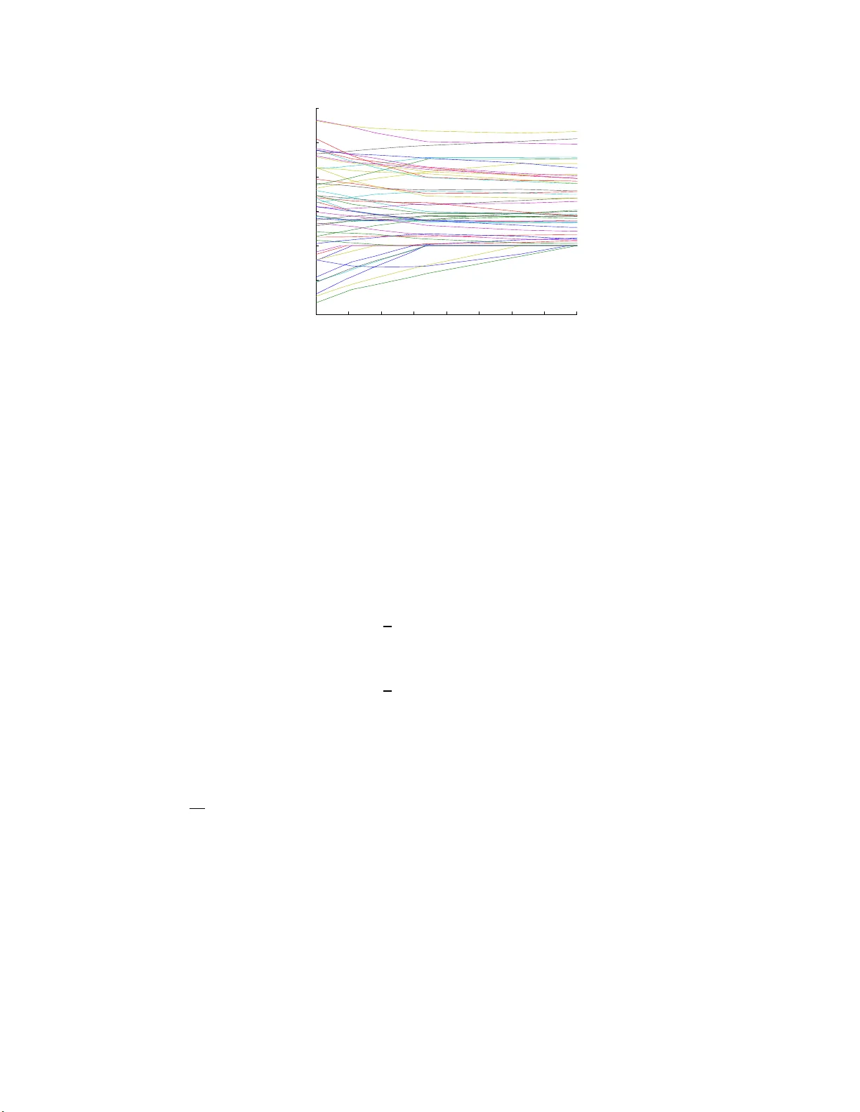
P ath F ollo wi ng in the Exact P enalt y Meth o d of Conv ex Programming Hua Zhou Departmen t of Statistics 2311 Stinson D riv e North Carolina Stat e Univ ersit y Raleigh, NC 27 695-820 3 E-mail: h ua zhou@ncsu.edu Kenneth Lange Departmen ts of Biomathematics, Human Genetics, and Statistics Univ ersit y of California Los Angeles, CA 9009 5-1766 E-mail: klange@ucla.edu Octob er 30, 201 8 Abstract Classica l p enalty metho d s solve a sequence of unconstrained problems that put greater and greater stress on meeting th e constraints. In the limit as the p enalty constant ten ds to ∞ , one reco vers the constrained solution. In the ex act p enalty meth od , squ ared p enalties are replaced by absolute v alue p enalties, and the solution is reco vered for a finite v alue of the p enalty constant. In practice, the kinks in the p enalty and the unkn ow n magnitude of the p en alt y constan t p reven t wide application of the exact p enalty metho d in nonlinear programming. I n this article, we examine a strategy of path follo wing con- sisten t with the exact p en alt y metho d. Instead of p erforming optimization at a single p enalt y constant, w e trace t h e solution as a contin uous function of the p enalty constan t. Thus, path follo wing starts at the unconstrained solution and follo ws the solution path as the p enalty constant increases. In the pro cess, the solution path hits, slides along, and exits from the v arious constraints. F or quadratic programming, the solution path is piecewise linear and takes large jumps from constraint to constraint. F or a gen- eral conv ex program, the solution path is piecewise smo oth, and path follo wing op erates by numerically solving an ordinary differential equation segment by segmen t . Our d ivers e app lications to a) pro jection onto a conv ex set, b) n onnegative least squares, c) quadratically constrained quadratic programming, d) geometric programming, and e) semidefinite programming illustrate the mechanics and p otential of path follo wing. The final detour to image denoising demonstrates the relev ance of path follo wing to regularized estimation in inv erse p roblems. I n regularized estimation, one follo ws the solution p ath as the p enalty constan t decreases from a large v alue. Keywords: constrained con vex optimization, exact p enalty , geometric programming, ordinary differ- entia l equation, quadratically constrained quadratic programming, regularization, semidefin ite p rogram- ming 1 In tro d uction Penalties and ba rriers are b oth p otent devices for solv ing constrained optimization problems (Bo yd a nd V andenberghe, 2004; F orsgren et al., 2002; Luenber ger and Y e, 2008; Nocedal and W r ight, 20 0 6; Ruszczy ´ nski, 2006; Zangwill, 1967). The g eneral idea is to repla c e hard constr aints by p ena lties or barriers and then exploit the well-oiled machinery for solv ing unconstrained pr oblems. Penalt y metho ds op era te on the exter ior of the feasible regio n 1 Researc h suppor ted in part by USPHS grants GM53275 and MH59490 to KL, R01 HG006139 to KL and HZ, and NCSU FRPD grant to HZ. 1 and bar rier metho ds on the interior. The strength of a pena lty or barrier is deter mined by a tuning constant. In classica l p enalty metho ds, a single global tuning constant is gradua lly sent to ∞ ; in ba rrier metho ds, it is gr adually sent to 0 . E ither strateg y gener ates a sequenc e of solutions tha t conv er ges in practice to the solution of the origina l cons tr ained o ptimization problem. Barrier metho ds a re now generally conceded to offer a b etter approa ch to solving conv ex progra ms than pena lty metho ds. Application of lo g ba r riers a nd ca refully co ntrolled versions of Newton’s metho d make it po ssible to fo llow the cen tral path r eliably and q uickly to the constrained minimum (Boyd and V a ndenberghe, 2004). Nonetheless , p enalty metho ds should not b e r uled o ut. Augmented Lag rangia n methods (Hestenes, 1975) and ex act p enalty metho ds (No cedal a nd W right, 2 006) are p otentially comp etitive with interior po int metho ds for smo oth co nv ex pr ogra mming problems. Both metho ds hav e the adv antage that the solution of the co nstrained pro blem kicks in for a finite v alue o f the p enalty consta nt . This avoids pr oblems of ill conditioning as the pe na lty constant tends to ∞ . The disadv antage of exact p enalties ov er tr a ditional quadratic p enalties is lack of differentiabilit y of the p enalized ob jective function. In the current pa pe r , we ar g ue tha t this imp ediment ca n be fines sed by path following. O ur path following metho d s tarts at the unco nstrained solution and follows the solution path a s the pe na lty co nstant increases. In the pro cess, the solution pa th hits, exits, and slides along the v arious constra int b oundar ies. T he path its e lf is piecewise s mo oth with kinks a t the b oundary hitting and escap e times. One a dv ances along the path by numerically solving a differential equa tion for the Lagr ange m ultiplier s of the p e nalized problem. In the sp ecia l case o f qua dratic progr amming with affine constraints, the so lution path is piecewis e linear, and o ne ca n easily anticipate entire path segments (Zhou and Lange, 2011b). This sp ecial case is intimately rela ted to the linear complementarity pro blem (Cottle et al., 1992) in optimization theor y . Homotopy (contin uation) metho ds for the so lution of nonlinear equa tions and optimization pro blems hav e b een purs ue d for many years and enjoy ed a v ar iety of successes (No cedal and W right, 200 6; W atson, 1986, 0 001; Zangwill a nd Ga rcia, 1981). T o our knowledge, how ever, ther e has b een no exploratio n of path following as a n implementation of the exact pena lty metho d. Our mode s t goa l here is to assess the feas ibility and versatility of exact pa th following for constrained optimiza tion. Comparing its p erforma nce to existing metho ds, particular ly the interior p oint metho d, is pr o bably b est left for later, mo r e practically or iented pap ers. In our exp erience, co ding the a lgorithm is straightforward in Matlab. The rich numerical resources of Ma tlab include differential eq uation solvers that a lert the us e r when certain ev e nts such as constr aint hitting and e s cap e o ccur. The r est of the pap er is or ganized as follows. Section 2 briefly reviews the exa ct p enalty metho d for optimization a nd inv estig ates sufficient conditions for uniquenes s and contin uity of the solutio n path. Section 2 3 de r ives the path following strategy for ge ne r al co nvex pro grams, with par ticular attention to the s pe cial cases of quadratic progra mming and conv ex optimization with affine constra int s . Section 4 presents v arious applications of the path alg orithm. Our mos t elab or ate example demonstrates the relev ance of pa th following to reg ularized estimatio n. The particula r problem treated, image denois ing, is typical of many inv ers e problems in applied ma thema tics and statistics Zho u and W u (201 1). In such problems o ne follows the solution path as the p ena lty constant de c r eases. Finally , Section 5 discusses the limitations of the path algorithm and hints at future ge ne r alizations. 2 Exact P enalt y Metho ds In this pap er we co nsider the conv ex progr amming pr oblem o f minimizing the conv ex ob jectiv e function f ( x ) sub ject to r a ffine eq ua lity constraints g i ( x ) = 0 and s conv ex inequality constra ints h j ( x ) ≤ 0 . W e will further assume that f ( x ) and the h j ( x ) ar e twice different iable. The differential d f ( x ) is the row vector of pa rtial der iv atives of f ( x ); the g radient ∇ f ( x ) is the transp ose of d f ( x ). The second differe nt ia l d 2 f ( x ) is the Hessian ma trix of second partial deriv atives of f ( x ). Similar conv entions hold for the differentials of the constra int functions. Exact pe na lty metho ds (No cedal and W right, 20 0 6; Ruszczy ´ nski, 200 6) minimize the surrog ate function E ρ ( x ) = f ( x ) + ρ r X i =1 | g i ( x ) | + ρ s X j =1 max { 0 , h j ( x ) } . (1) This definition of E ρ ( x ) is meaningful r egardle s s o f whether the co ntributing functions are conv ex. If the progra m is co nv ex, then E ρ ( x ) is itself co nv ex. It is in ter esting to compar e E ρ ( x ) to the La grang ia n function L ( x ) = f ( x ) + r X i =1 λ i g i ( x ) + s X j =1 µ j h j ( x ) , which captures the b ehavior of f ( x ) near a constr ained lo cal minimum y . The Lag rangia n s a tisfies the sta- tionarity condition ∇L ( y ) = 0 ; its inequality multipliers µ j are nonnegative and satisfy the complementary slackness conditions µ j h j ( y ) = 0. In an ex act p enalty metho d o ne takes ρ > max {| λ 1 | , . . . , | λ r | , µ 1 , . . . , µ s } . (2) This choice crea tes the fav o rable cir cumstances L ( x ) ≤ E ρ ( x ) for all x L ( z ) ≤ f ( z ) = E ρ ( z ) for a ll feasible z L ( y ) = f ( y ) = E ρ ( y ) for y o ptimal with pr ofound consequences. As the next prop os ition proves, minimizing E ρ ( x ) is effective in minimizing f ( x ) sub ject to the constra ints. 3 Prop ositi on 2 .1. Supp ose t he obje ctive function f ( x ) and the c onstr aint functions ar e t wic e differ entiable and satisfy the L agr ange multiplier rule at t he lo c al minimum y . If ine quality (2) holds and v ∗ d 2 L ( y ) v > 0 for every ve ctor v 6 = 0 satisfying dg i ( y ) v = 0 and dh j ( y ) v ≤ 0 for al l active ine quality c onstr aints, then y furn ishes an unc onstra ine d lo c al minimum of E ρ ( x ) . F or a c onvex pr o gr am s atisfying Slater’s c onstr aint qualific ation and ine quality (2), y is a minimum of E ρ ( x ) if and only if y is a minimum of f ( x ) subje ct to the c onstr aints. N o differ entiability assumptions ar e r e qu ir e d for c onvex pr o gr ams. Pr o of. The conditions imp osed on the quadratic for m v ∗ d 2 L ( y ) v are well-kno wn sufficient conditions for a lo cal minim um. Theo rems 6.9 a nd 7.21 of the reference Rus zczy ´ nski (20 06) prove a ll o f the foreg oing assertions . As previously stressed, the exact p enalty method turns a constrained optimization pro blem in to an uncon- strained minimization pro blem. F urthermore, in co nt r ast to the quadratic penalty metho d (Noceda l and W rig ht , 2006, Section 17.1), the constr ained so lution in the exact metho d is achiev ed for a finite v alue of ρ . Despite these adv antages, minimizing the surroga te function E ρ ( x ) is complica ted. F o r one thing, it is no longer globally differentiable. F or another , one m us t minimize E ρ ( x ) along an incre a sing s equence ρ n bec ause the Lagra ng e multipliers (2) are usually unknown in adv ance. These hurdles have pre ven ted wide a pplication of exact p enalty metho ds in conv ex prog ramming. As a prelude to our deriv ation of the path following a lg orithm for conv ex prog rams, we r ecord several prop erties of E ρ ( x ) that mitigate the failure of differentiabilit y . Prop ositi on 2 .2. The surr o gate function E ρ ( x ) is incr e asing in ρ . F urthermor e, E ρ ( x ) is strictly c onvex for one ρ > 0 if and only if it is strictly c onvex for al l ρ > 0 . Likewise, it is c o er cive for one ρ > 0 if and only if is c o er cive for al l ρ > 0 . Final ly, if f ( x ) is st rictly c onvex (or c o er cive), then al l E ρ ( x ) ar e strictly c onvex (or c o er cive). Pr o of. The fir st as s ertion is obvious. F or the s econd a ssertion, consider mor e gene r ally a finite family u 1 ( x ) , . . . , u q ( x ) of conv ex functions, and suppo se a linear combination P q k =1 c k u k ( x ) with po sitive co effi- cients is strictly convex. It suffices to pr ov e that a ny other linear combination P q k =1 b k u k ( x ) with pos itive co efficients is strictly conv ex. F or any t wo po ints x 6 = y and any scala r α ∈ (0 , 1), we hav e u k [ α x + (1 − α ) y ] ≤ αu k ( x ) + (1 − α ) u k ( y ) . (3) Since P q k =1 c k u k ( x ) is stric tly co nv ex, stric t inequality must ho ld fo r at least one k . Hence, m ultiplying inequality (3) by b k and adding g ives q X k =1 b k u k [ α x + (1 − α ) y ] < α q X k =1 b k u k ( x ) + (1 − α ) q X k =1 b k u k ( y ) . 4 The third a ssertion follows fro m the fact that a conv ex function is co ercive if a nd only if its r estriction to each half-line is co erc ive (Bertsek as, 2 003, Pr op osition 3.2.2 ). Given this result, suppo se E ρ ( x ) is co ercive, but E ρ ∗ ( x ) is not co er cive. Then there exists a p oint x , a direction v , and a seq uence of scala rs t n tending to ∞ such that E ρ ∗ ( x + t n v ) is b ounded ab ove. This req uires the sequence f ( x + t n v ) and ea ch of the sequences | g i ( x + t n v ) | and max { 0 , h j ( x + t n v ) to r emain b ounded ab ove. But in this circumstance the sequence E ρ ( x + t n v ) als o remains b ounded a b ove. The final tw o a ssertions are obvious. 3 The P ath F ollo wing Algorithm In this section, w e take a different p o int of view. Instead of minimizing E ρ ( x ) for an increasing sequence ρ n , we study how the solution x ( ρ ) changes contin uously with ρ and devise a path fo llowing str ategy sta rting from ρ = 0. F or some finite v alue of ρ , the path lo cks in on the s olution o f the or iginal conv ex progr am. In re gularized statistical estimation and inv erse problems, the primar y go a l is to s elect r elev ant predictor s rather than to find a co nstrained so lutio n. Thus, the en tir e solution pa th commands more in ter est than a ny single po int along it (Efr on et al., 2 004; Osb orne et al., 2 000; Tibshirani and T aylor, 2011; Zhou and La nge, 2011b; Zhou and W u, 20 11). Although our theory will fo cus on cons trained estimation, r eaders s hould b ear in mind this second application a rea of path following. The path algorithm relies critically o n the fir s t o rder optimality condition that characterizes the o ptimu m po int of the c o nv ex function E ρ ( y ). Prop ositi on 3.1. F or a c onvex pr o gr am, a p oint x = x ( ρ ) minimizes the function E ρ ( y ) if and only if x satisfies the stationarity c ondition 0 = ∇ f ( x ) + ρ r X i =1 s i ∇ g i ( x ) + ρ s X j =1 t j ∇ h j ( x ) (4) for c o efficient sets { s i } r i =1 and { t j } s j =1 . These sets c an b e char acterize d as s i ∈ {− 1 } g i ( x ) < 0 [ − 1 , 1] g i ( x ) = 0 { 1 } g i ( x ) > 0 and t j ∈ { 0 } h j ( x ) < 0 [0 , 1] h j ( x ) = 0 { 1 } h j ( x ) > 0 . (5) At most one p oint achieves t he minimum of E ρ ( y ) for a given ρ when E ρ ( y ) is strictly c onvex. Pr o of. According to F ermat’s rule, x minimizes E ρ ( y ) if and only if 0 b elong s to the sub differential ∂ E ρ ( x ) of E ρ ( y ). T o der ive the sub differential dis play ed in equations (4) and (5), one a pplies the addition and chain rules of the c o nv ex calculus. The sets defining the p os sible v alues o f s i and t j are the subdiffer e nt ia ls of the functions | s | and t + = max { t, 0 } , res p e c tively . F o r mo re deta ils see Theo rem 3 .5 a nd ancillar y mater ial in the bo ok (Ruszczy ´ nski, 200 6). Finally , it is well known that stric t conv exity guara nt e es a unique minimum. 5 T o sp eak c o herently of so lution paths, o ne must v alidate the existence , uniqueness, and contin uity of the solution x ( ρ ) to the system of equations (1). Uniqueness follows from stric t c onv exity as already noted. Existence and contin uity a re more subtle. Prop ositi on 3.2 . If E ρ ( y ) is strictly c onvex and c o er cive, t hen the solution p ath x ( ρ ) of e quation (1 ) exists and is c ontinuous in ρ . If the gr adient ve ctors { ∇ g i ( x ) : g i ( x ) = 0 } ∪ {∇ h j ( x ) : h j ( x ) = 0 } of the active c onstr aints ar e line arly indep endent at x ( ρ ) for ρ > 0 , then the c o efficients s i ( ρ ) and t j ( ρ ) ar e unique and c ontinuous ne ar ρ as wel l. Pr o of. In accord with Prop o sition 2.2, we assume that either f ( x ) is s trictly co nv ex and co ercive or restrict our attention to the op e n interv al (0 , ∞ ). Consider a s ubin ter v al [ a, b ] and fix a p oint x in the common domain of the functions E ρ ( y ). The co ercivity of E a ( y ) and the inequalities E a [ x ( ρ )] ≤ E ρ [ x ( ρ )] ≤ E ρ ( x ) ≤ E b ( x ) demonstrate tha t the solutio n vector x ( ρ ) is b ounded ov er [ a, b ]. T o prov e contin uity , supp ose tha t it fails for a given ρ ∈ [ a, b ]. Then there exists an ǫ > 0 and a sequence ρ n tending to ρ such k x ( ρ n ) − x ( ρ ) k 2 ≥ ǫ for all n . Since x ( ρ n ) is b ounded, w e ca n pas s to a subsequenc e if necessa ry and assume that x ( ρ n ) conv erg es to some p oint y . T aking limits in the inequa lity E ρ n [ x ( ρ n )] ≤ E ρ n ( x ) demonstrates that E ρ ( y ) ≤ E ρ ( x ) for all x . Because x ( ρ ) is unique, we reach the contradictory conclusions k y − x ( ρ ) k 2 ≥ ǫ a nd y = x ( ρ ). V erification of the s econd claim is defer red to per mit further discus sion of path following. The claim says that an active constr a int ( g i ( x ) = 0 or h j ( x ) = 0) remains a ctive until its co efficient hits an endp oint of its sub differ ential. B ecause the solution path is, in fact, piecewise smo o th, one can follow the co efficient path by numerically s olving an or dinary differential equatio n (O DE ). Our path following algor ithm works s e g ment-b y-segment. Along the pa th we keep track of the following index sets N E = { i : g i ( x ) < 0 } N I = { j : h j ( x ) < 0 } Z E = { i : g i ( x ) = 0 } Z I = { j : h j ( x ) = 0 } (6) P E = { i : g i ( x ) > 0 } P I = { j : h j ( x ) > 0 } determined by the signs of the constraint functions. F or the s ake of simplicity , ass ume that at the b eginning of the current segment s i do es no t equal − 1 or 1 when i ∈ Z E and t j do es no t equal 0 or 1 when j ∈ Z I . In other words, the co efficients o f the a ctive cons tr aints o ccur on the interior o f their sub differentials. Let us show in this circumstance that the so lution path can b e extended in a smo oth fashion. Our plan o f attack is to repa rameterize by the Lagra nge multipliers for the active constraints. Thus, set λ i = ρs i for i ∈ Z E and 6 ω j = ρt j for j ∈ Z I . The multipliers satisfy − ρ < λ i < ρ and 0 < ω j < ρ . The stationa r ity condition now reads 0 = ∇ f ( x ) − ρ X i ∈N E ∇ g i ( x ) + ρ X i ∈P E ∇ g i ( x ) + ρ X j ∈P I ∇ h j ( x ) + X i ∈Z E λ i ∇ g i ( x ) + X j ∈Z I ω j ∇ h j ( x ) . T o this we concatenate the co nstraint equations 0 = g i ( x ) for i ∈ Z E and 0 = h j ( x ) for j ∈ Z I . F or conv e nience now define U Z ( x ) = dg Z E ( x ) dh Z I ( x ) , u ¯ Z ( x ) = − X i ∈N E ∇ g i ( x ) + X i ∈P E ∇ g i ( x ) + X j ∈P I ∇ h j ( x ) . In this no ta tion the stationa rity equation can b e r ecast as 0 = ∇ f ( x ) + ρ u ¯ Z ( x ) + U t Z ( x ) λ ω . Under the a ssumption that the matrix U Z ( x ) has full r ow rank , one can solve for the Lag range multipliers in the for m λ Z E ω Z I = − [ U Z ( x ) U t Z ( x )] − 1 U Z ( x ) [ ∇ f ( x ) + ρ u ¯ Z ( x )] . (7) Hence, the mu ltiplier s ar e unique. Con tinuit y of the multipliers is a co nsequence of the co nt inuit y of the solution vector x ( ρ ) and all functions in sight on the right-hand side of equatio n (7). This o bserv ation completes the pro of of Pr op osition 3.2. Collectively the stationarity a nd active co ns traint equa tions can be written as the vector equa tion 0 = k ( x , λ , ω , ρ ). T o solve for x , λ a nd ω in terms of ρ , w e apply the implicit function theorem (Lange, 2 004; Magnus and Neudeck e r, 19 9 9). This r equires calculating the differential of k ( x , λ , ω , ρ ) with res pe c t to the underlying depe ndent v ar iables x , λ , and ω and the indep endent v ariable ρ . Because the e q uality constraints are affine, a br ief calculatio n gives ∂ x , λ , ω k ( x , λ , ω , ρ ) = d 2 f ( x ) + ρ P j ∈P I d 2 h j ( x ) + P j ∈Z I ω j d 2 h j ( x ) U t Z ( x ) U Z ( x ) 0 ∂ ρ k ( x , λ , ω , ρ ) = u ¯ Z ( x ) 0 . The matrix ∂ x , λ , ω k ( x , λ , ω , ρ ) is nonsing ula r when its uppe r-left blo ck is po sitive definite and its low er-left blo ck has full row rank (Lange, 2010, Pr op osition 11.3 .2). Given that it is no ns ingular, the implicit function theorem applies, and we c an in principle so lve for x , λ a nd ω in ter ms of ρ . More imp ortantly , the implicit function theorem supplies the deriv ative d dρ x λ Z E ω Z I = − ∂ x , λ , ω k ( x , λ , ω , ρ ) − 1 ∂ ρ k ( x , λ , ω , ρ ) , (8) which is the key to path fo llowing. W e summar ize our findings in the next pr o p osition. 7 Prop ositi on 3. 3. Supp ose the su r ro gate funct ion E ρ ( y ) is st r ictly c onvex and c o er cive. If at the p oint x ( ρ 0 ) t he matrix ∂ x , λ , ω k ( x , λ , ω , ρ ) is nonsingular and the c o efficient of e ach active c onstr aints o c curs on the interior of its sub differ ential, then the solution p ath x ( ρ ) and L agr ange mu ltipliers λ ( ρ ) and ω ( ρ ) satisfy the differ ential e quation (8) in the vicinity of x ( ρ 0 ) . In practice one tra ces the solution pa th along the current time s egment until either an inactive co nstraint bec omes active o r the co efficient of an a ctive constraint hits the b oundary of its sub differential. The e arliest hitting time or escap e time over a ll constraints determines the duratio n o f the current segment. When the hitting time for an ina ctive constra int o ccurs firs t, we mov e the constra int to the a ppropriate active s et Z E or Z I and keep the other constraints in pla ce. Similarly , when the esca p e time for an active constra int o ccurs first, we mov e the c onstraint to the appropria te inactive set and keep the other cons traints in pla ce. In the second scenar io, if s i hits the v alue − 1, then we move i to N E ; If s i hits the v alue 1, then we mov e i to P E . Similar comments apply when a co efficient t j hits 0 or 1 . Once this mov e is executed, we commence path following along the new segment. Path following contin ues un til for sufficiently larg e ρ , the sets N E , P E , and P I are exhausted, u ¯ Z = 0 , and the solution vector x ( ρ ) sta bilizes. Our previous pap er (Zhou and Lange, 2011b) sugges ts remedies in the very rar e situations wher e escap e times coincide. Path following simplifies considera bly in t wo sp ecial cases. Co nsider conv e x quadratic progra mming with ob jective function f ( x ) = 1 2 x t A x + b t x and equality constraints V x = d and inequa lity co nstraints W x ≤ e , where A is p os itive semi-definite. The ex act p enalized o b jective function b eco mes E ρ ( x ) = 1 2 x t A x + b t x + ρ s X i =1 | v t i x − d i | + ρ t X j =1 ( w t j x − e j ) + . Since b oth the equa lity and inequality constraints a re affine, their second der iv atives v anish. B oth U Z and u ¯ Z are constant on the curre nt path s egment, and the path x ( ρ ) satis fie s d dρ x λ Z E ω Z I = − A U t Z U Z 0 − 1 u ¯ Z 0 . (9) This implies that the solution pa th x ( ρ ) is piecewise linear. Our previous pa p e r (Zhou and Lange, 2 011b) is devoted en tir ely to this sp ecia l class of pro blems and highlights many statistical applica tions. On the next rung o n the ladder of generality are convex progra ms with affine co ns traints. F or the exact surrog ate E ρ ( x ) = f ( x ) + ρ s X i =1 | v t i x − d i | + ρ t X j =1 ( w t j x − e j ) + , the matrix U Z and vector u ¯ Z are still constant alo ng a pa th segment. The relev ant differ e nt ia l equatio n 8 bec omes d dρ x λ Z E ω Z I = − d 2 f ( x ) U t Z U Z 0 − 1 u ¯ Z 0 . (10) There ar e t wo appro aches for co mputing the right-hand side of equation (10). When A = d 2 f ( x ) is p os itive definite and B = U Z has full row ra nk, the relev ant inverse amounts to A B t B 0 − 1 = A − 1 − A − 1 B t [ B A − 1 B t ] − 1 B A − 1 A − 1 B t [ B A − 1 B t ] − 1 [ B A − 1 B t ] − 1 B A − 1 − [ B A − 1 B t ] − 1 . The n umerica l cost of c o mputing the in verse scales a s O ( n 3 )+ O ( |Z | 3 ). When d 2 f ( x ) is a constant , the inverse is co mputed once. Sequentially up dating it fo r differe nt active sets Z is then co nv eniently or ganized aro und the s weep o p erator of computatio na l statistics (Zhou and La nge, 201 1b). F or a genera l conv ex function f ( x ), every time x changes, the in verse must be recomputed. This burden plus the cost of computing the e ntries of d 2 f ( x ) slow the path algor ithm for ge neral conv e x pro ble ms . In ma ny applications f ( x ) is conv e x but not necessar ily stric tly c o nv ex. One can circumv ent problems in inv erting d 2 f ( x ) by r eparameter izing (No cedal and W rig ht , 20 06). F or the sake of simplicity , suppo se that all of the constra int s are a ffine and that U Z has full r ow ra nk. T he set of p oints x sa tisfying the active constraints ca n b e written as x = w + Y y , where w is a par ticular solution, y is free to v ary , a nd the columns of Y ∈ R n × ( n −|Z | ) span the n ull space of U Z and hence are or tho gonal to the rows o f U Z . Under the null s pa ce repar a meterization, d x dρ = Y d y dρ . F urthermor e , Y t d 2 f ( x ) Y = d 2 y f ( w + Y y ) Y t u ¯ Z ( x ) = ∇ y h − ρ X i ∈N E g i ( w + Y y ) + ρ X i ∈P E g i ( w + Y y ) + ρ X j ∈P I h j ( w + Y y ) i . It follows tha t e quation (10) bec o mes d dρ y = − [ Y t d 2 f ( x ) Y ] − 1 Y t u ¯ Z d dρ x = − Y [ Y t d 2 f ( x ) Y ] − 1 Y t u ¯ Z . (11) Different ia ting equa tion (7) gives the m ultiplier deriv atives d dρ λ Z E ω Z I = − ( U Z U t Z ) − 1 U Z d 2 f ( x ) d x dρ + u ¯ Z . (12) The obvious adv antage o f using eq uation (11) is that the ma trix Y t d 2 f ( x ) Y can b e nonsingular when d 2 f ( x ) is sing ular. The c o mputational c o st of ev aluating the right-hand sides of equations (11) and (12 ) is O ([ n − |Z | ] 3 ) + O ( |Z | 3 ). When n − |Z | a nd |Z | a re small compared to n , this is an improvemen t ov er the cost O ( n 3 ) + O ( |Z | 3 ) of co mputing the right-hand side of equa tion (8). Balanced ag ainst this gain is 9 the requir e ment of finding a bas is of the null space of U Z . F ortunately , the matrix Y is cons tant ov er each path segment and in pr actice ca n b e computed by taking the Q R decomp osition of the a ctive constraint matrix U Z . A t each kink of the solution path, either one constr aint enters Z or one leaves. Ther efore, Y can be seq uent ially co mputed by standar d up dating a nd downdating formulas (Lawson and Hanson, 1987; Noc edal and W r ight, 2006). Which ODE (8) or (11) is prefer able dep ends on the sp ecific a pplication. When the loss function f ( x ) is not str ictly conv ex, for example when the n umber o f parameter s exce e ds the num b er of cases in regr ession, pa th following requires the ODE (1 1). In tere s ted reader s are referr ed to the b o o k (Noceda l and W rig ht , 20 06) for a more extended discussion of r ange-s pa ce versus null-space optimization metho ds. F or a ge ner al conv ex progra m, one ca n employ Euler ’s up da te x ( ρ + ∆ ρ ) λ ( ρ + ∆ ρ ) ω ( ρ + ∆ ρ ) = x ( ρ ) λ ( ρ ) ω ( ρ ) + ∆ ρ d dρ x ( ρ ) λ ( ρ ) ω ( ρ ) to adv ance the solution of the ODE (8 ). Euler’s for mula may b e inacc ur ate for ∆ ρ larg e. One can cor rect it by fixing ρ and p erforming one step o f Newton’s metho d to re-connect with the s olution path. This amounts to replacing the po sition-multiplier vector b y x λ ω − ∂ x , λ , ω k ( x , λ , ω , ρ ) − 1 k ( x , λ , ω , ρ ) . In practice, it is cer tainly easier a nd probably sa fer to rely o n ODE pa ck ages such as the ODE4 5 function in Ma tlab to adv ance the so lution of the O DE. 4 Examples of P ath F ollo wing Our exa mples ar e in tended to illuminate the mechanics o f path following and show ca se its versatility . As we emphasized in the intro duction, we forgo co mparisons with other metho ds. Compar isons dep end heavily on progra mming details and problem choices, so a premature study might well b e misleading. Example 4.1. Pr oje ct ion onto t he F e asible Re gion Finding a fea s ible po int is the initial stag e in many c onv ex prog rams. Dykstra’s alg o rithm (Dykstra, 1983; Deutsch, 20 01) w as designed precisely to s olve the pro blem of pro jecting a n exterior p oint onto the int er section of a finite num b er of closed conv ex sets. The pr o jection problem also yie lds to o ur g eneric path following algo rithm. Consider the toy example of pr o jecting a po int b ∈ R 2 onto the intersection of the closed unit ball and the clos ed half space x 1 ≥ 0 (La ng e, 2004). This is equiv alent to solving minimize f ( x ) = 1 2 k x − b k 2 sub ject to h 1 ( x ) = 1 2 k x k 2 − 1 2 ≤ 0 , h 2 ( x ) = − x 1 ≤ 0 . 10 The relev ant g radients and second differentials are ∇ f ( x ) = x − b , ∇ h 1 ( x ) = x , ∇ h 2 ( x ) = − 1 0 d 2 f ( x ) = d 2 h 1 ( x ) = I 2 , d 2 h 2 ( x ) = 0 . Path following star ts from the unconstraine d solution x (0) = b ; the direction of mov ement is deter mined by formula (8). F o r x ∈ { x : k x k 2 > 1 , x 1 > 0 } , the path d dρ x = − [(1 + ρ ) I 2 ] − 1 x = − 1 1 + ρ x heads tow ar d the o rigin. F or x ∈ { x : | x 2 | > 1 , x 1 = 0 } , the path d dρ x ω 2 = − 1 + ρ 0 − 1 0 1 + ρ 0 − 1 0 0 − 1 x 1 x 2 0 = − 1 1 + ρ 0 x 2 0 also heads toward the or ig in. F or x ∈ { x : k x k 2 > 1 , x 1 < 0 } , the pa th d dρ x = − [(1 + ρ ) I 2 ] − 1 x 1 − 1 x 2 = − 1 1 + ρ x 1 − 1 x 2 . heads tow ar d the p o int (1 , 0) t . F o r x ∈ { x : k x k 2 = 1 , x 1 < 0 } , the path d dρ x ω 1 = − 1 + ω 1 0 x 1 0 1 + ω 1 x 2 x 1 x 2 0 − 1 − 1 0 0 = − x 2 2 1+ ω 1 x 1 x 2 1+ ω 1 − x 1 is tangent to the circle. Finally , for x ∈ { x : k x k 2 < 1 , x 1 < 0 } , the path d dρ x = − I − 1 2 − 1 0 = 1 0 heads tow ar d the x 2 -axis. The left panel of Figur e 1 plo ts the vector field d dρ x at the time ρ = 0. The rig ht panel shows the so lution path for pro jection from the po ints ( − 2 , 0 . 5) t , ( − 2 , 1 . 5) t , ( − 1 , 2 ) t , (2 , 1 . 5) t , (2 , 0) t , (1 , 2) t , and ( − 0 . 5 , − 2) t onto the feas ible r egion. In pr o jecting the p oint b = ( − 1 , 2) t onto (0 , 1) t , the ODE45 solver o f Ma tlab ev aluates deriv atives at 19 different time p oints. Dykstra’s algor ithm by comparison takes ab out 30 itera tio ns to conv er g e (La ng e, 2004). Example 4.2. Nonne gative L e ast Squar es (NNLS) and Nonn e gative Matrix F actoriza t ion (NN MF) Non-negative matrix fac to rization (NNMF) is an alterna tive to pr inciple co mpo nent analysis a nd is useful in mo deling, compr essing, and interpreting nonnegative data s uch as obs erv ational co unt s and images . The articles (Berry et al., 2007; Lee and Seung , 1999, 2 001) discuss in detail estimation algor ithms and statistica l applications o f NNMF. The basic idea is to approximate an m × n data matrix X = ( x ij ) w ith nonnegative ent r ies by a pr o duct V W o f t wo low ra nk matrices V = ( v ik ) and W = ( w kj ) with nonneg ative entries. 11 −2 −1 0 1 2 −2 −1.5 −1 −0.5 0 0.5 1 1.5 2 x 1 x 2 −2 −1 0 1 2 −2 −1.5 −1 −0.5 0 0.5 1 1.5 2 x 1 x 2 Figure 1: Pro jectio n to the po sitive half disk. Left: Deriv atives a t ρ = 0 for pro jectio n onto the ha lf disc. Right: Pro jection tr a jector ie s fro m v arious initial p oints. Here V and W are m × r and r × n r esp ectively , with r ≪ min { m, n } . O ne v e r sion of NNMF minimizes the criterion f ( V , W ) = k X − V W k 2 F = X i X j x ij − X k v ik w kj 2 , (13) where k · k F denotes the F ro b enius nor m. In a typical imaging pr o blem, m (nu mber of images) might range from 1 0 3 to 10 4 , n (num b er of pixels per imag e) might surpass 10 4 , and a rank r = 50 approximation might adequately capture X . Minimization of the o b jective function (13) is nontrivial be cause it is not jointly conv ex in V and W . Multiple lo c al minima are pos sible. The well-known multiplicative algo rithm (Lee a nd Seung, 1999, 2001) enjoys the descent proper ty , but it is not guara nteed to conv erg e to ev en a lo ca l minim um (Ber ry et a l., 2007). An alter native algor ithm that ex hibits b etter conv er gence is alternating le a st squa res (ALS). In up dating W with V fixed, ALS solves the n separa ted no nnegative least squar e (NLS) problems min w j k x j − V w j k 2 2 sub ject to w j ≥ 0 , (14) where x j and w j denote the j -th c o lumns of the corres p o nding matrices. Similarly , in up dating V with W fixed, ALS solves m separa ted NNLS problems. The unconstra ined solution W (0) = ( V t V ) − 1 V t X o f W for fixed V requires just one QR decomp osition of V or one Cholesky decomp os itio n o f V t V . The exa ct path algo rithm for s olving the subpr oblem problem (14) commences with W (0). If W ( ρ ) s ta bilizes with just a few zer os, then the path a lgorithm ends quickly and is extremely efficient. F or a NNLS proble m, the path is piecewise linea r , and one can straightforwardly pro ject the pa th to the next hitting or es c ap e time using the sweep op er a tor (Zhou and Lange, 2011b). Figure 2 shows a typical piecewise linear path for a problem 12 0 0.5 1 1.5 2 2.5 3 3.5 4 −1 −0.5 0 0.5 1 1.5 2 ρ x i ( ρ ) Figure 2: Piecewise linea r paths of the regr ession co efficie nts for a NNLS problem with 50 predicto rs. with r = 50 predictors. Each pro jection to the next even t requires 2 r 2 flops. The num b er o f path s egments (even ts) roughly sc a les a s the num b er of negative co mpo nents in the unconstr a ined solution. Example 4.3. Quadr atic al ly Constr aine d Quadr atic Pr o gr amming (Q CQP) Example 4.1 is a sp ecia l cas e o f quadra tically constrained quadratic pr ogra mming (QCQP). In conv ex QCQP (Boyd and V a ndenberghe, 2004, Section 4.4), one minimizes a co nvex qua dratic function ov er an int er section of ellipsoids a nd affine subspa ces. Mathematically , this amounts to the pr oblem minimize f ( x ) = 1 2 x t P 0 x + b t 0 x + c 0 sub ject to g i ( x ) = a t i x − d i = 0 , i = 1 , . . . , r h j ( x ) = 1 2 x t P j x + b t j x + c j ≤ 0 , j = 1 , . . . , s, where P 0 is a p ositive definite ma trix and the P j are p ositive semidefinite ma trices. O ur a lgorithm starts with the unconstra ined minimum x (0) = − P − 1 0 b 0 and pro ceeds a long the path determined by the deriv ative d dρ x λ Z E ω Z I = − P 0 + ρ P j ∈P I P j + P j ∈Z I ω j P j U t Z ( x ) U Z ( x ) 0 − 1 u ¯ Z ( x ) 0 , where U Z ( x ) has rows a t i for i ∈ Z E and ( P j x + b j ) t for j ∈ Z I , and u ¯ Z ( x ) = − X i ∈N E a i + X i ∈P E a i + X i ∈P I ( P j x + b j ) . Affine inequality co nstraints can b e accommo dated by s etting one or mor e of the P j equal to 0 . 13 −2 −1 0 1 2 3 −2 −1.5 −1 −0.5 0 0.5 1 1.5 2 2.5 3 x 1 x 2 sol path objective constraint Figure 3: T ra jectory of the exact pena lt y path algo rithm for a QC Q P problem (15). The solid lines ar e the contours of the ob jectiv e function f ( x ). The dashed lines ar e the co ntours of the constraint functions h j ( x ). As a numerical illustra tion, consider the biv ariate problem minimize f ( x ) = 1 2 x 2 1 + x 2 2 − x 1 x 2 + 1 2 x 1 − 2 x 2 sub ject to h 1 ( x ) = x 1 − 1 2 2 + x 2 2 − 1 ≤ 0 (15) h 2 ( x ) = x 1 + 1 2 2 + x 2 2 − 1 ≤ 0 h 3 ( x ) = x 2 1 + x 2 − 1 2 2 − 1 ≤ 0 . Here the feas ible region is g iven by the intersection o f three disks with centers (0 . 5 , 0) t , ( − 0 . 5 , 0) t , a nd (0 , 0 . 5) t , resp ectively , and a co mmon ra dius of 1. Figur e 3 displays the solution tra jectory . Star ting from the unconstrained minimum x (0) = (1 , 1 . 5) t , it hits, slides along, and exits tw o circ le s b efore its jour ney e nds at the cons tr ained minimum (0 . 059 , 0 . 829) t . The ODE45 solver of Ma tl ab ev aluates deriv atives a t 72 time po ints alo ng the path. Example 4.4. Ge ometric Pr o gr amming As a branch of conv ex optimization theor y , geometr ic pr ogramming stands just behind linea r and quadratic pr o gramming in imp ortance (Boyd et al., 200 7; Eck e r, 1 9 80; Peressini et al., 1988; Peterson, 19 76). It ha s a pplications in chemical equilibrium problems (Passy and Wilde, 1968), structural mechanics (Eck er, 1980), digit circuit design (Boyd et al., 200 5), max imum likelihoo d estimation (Mazumdar a nd Jefferson, 1983), sto chastic pro ce s ses (F eigin and Passy, 19 81), and a host of other s ub jects (Boyd et a l., 2007; Eck er, 14 1980). Geometric prog ramming deals with p osy nomials, which ar e functions of the form f ( x ) = X α ∈ S c α n Y i =1 x α i i = X α ∈ S c α e α t y = f ( y ) . (16) In the left-hand definition of this equiv alent pair of definitions, the index set S ⊂ R n is finite, a nd a ll co- efficients c α and all comp onents x 1 , . . . , x n of the ar gument x of f ( x ) are p ositive. The p ossibly fractional powers α i corres p o nding to a par ticular α may b e p ositive, nega tive, or zero. F or instance, x − 1 1 + 2 x 3 1 x − 2 2 is a po synomial o n R 2 . In geometric progra mming, one minimizes a p o synomial f ( x ) sub ject to p osynomia l inequality constraints o f the for m h j ( x ) ≤ 1 for 1 ≤ j ≤ s . In some versions of geometric pro gramming, equality constraints of monomial t y pe a re per mitted (Boyd et al., 2 007). The right-hand definition in equa- tion (16) in vokes the exp onential repa r ameterizatio n x i = e y i . This simple transforma tion has the adv antage of rendering a geometr ic pro gram conv ex . In fact, any p osy no mial f ( y ) in the exp o nent ia l parameter ization is log-co nvex and therefore conv ex. The concise representations ∇ f ( y ) = X α ∈ S c α e α t y α , d 2 f ( y ) = X α ∈ S c α e α t y αα t of the g radient and the seco nd different ia l ar e helpful in b oth theory and computatio n. Without loss of ge nerality , one can rep ose ge o metric progra mming as minimize ln f ( y ) sub ject to ln g i ( y ) = 0 , 1 ≤ i ≤ r (17) ln h j ( y ) ≤ 0 , 1 ≤ j ≤ s, where f ( y ) and the h j ( y ) ar e p osynomials and the equality constr a ints ln g i ( y ) ar e affine. In this ex po nential parameteriza tion setting, it is easy to state ne c e ssary a nd s ufficient conditions for strict conv exity and co erciveness. Prop ositi on 4 .5. The obje ct ive function f ( y ) in the ge ometric pr o gr am (17) is strictly c onvex if and only if the subsp ac e sp anne d by the ve ctors { α } α ∈ S is al l of R n ; f ( y ) is c o er cive if and only if the p olar c one { z : z t α ≤ 0 for al l α ∈ S } r e duc es to the origin 0 . Equivalently, f ( y ) is c o er cive if the origin 0 b elongs to the interior of the c onvex hul l of the set S . Pr o of. These claims a re prov ed in detail in our pap er (Zhou and Lange, 2 0 11a). According to Pro po sitions 2.1 and 3.2, the strict conv exity and co erciveness of f ( y ) g uarantee the unique- ness and contin uity of the so lution path in y . This in turn implies the uniqueness and contin uity of the solution path in the orig inal pa rameter vector x . The pa th directions a re related by the chain rule d dρ x i ( ρ ) = dx i dy i d dρ y i ( ρ ) = x i d dρ y i ( ρ ) . 15 1 1.2 1.4 1.6 1.8 2 1 1.1 1.2 1.3 1.4 1.5 1.6 1.7 1.8 1.9 2 1 1 1 1 1.25 1.25 1.25 1.5 1.5 1.5 x 1 x 2 sol path objective constraint Figure 4: T ra jecto ry o f the exac t pena lt y path algor ithm for the geometric pro gramming problem (18). The solid lines a re the co ntours of the ob jective function f ( x ). The dashed lines ar e the contours of the constra int function h ( x ) a t le vels 1, 1.25, and 1.5. As a concrete exa mple, consider the pr oblem minimize x − 3 1 + 3 x − 1 1 x − 2 2 + x 1 x 2 (18) sub ject to 1 6 x 1 / 2 1 + 2 3 x 2 ≤ 1 , x 1 > 0 , x 2 > 0 . It is ea sy to chec k tha t the vectors { ( − 3 , 0) t , ( − 1 , − 2) t , (1 , 1) t } span R 2 and generate a co nvex hull strictly containing the orig in 0 . There fo re, f ( y ) is strictly co nv ex and co ercive. It achieves its unco nstrained minim um at the p oint x (0) = ( 5 √ 6 , 5 √ 6) t , or equiv alently y (0) = (ln 6 / 5 , ln 6 / 5) t . T o solve the constr ained minimization problem, we follow the path dictated by the rev ised g eometric program (17 ). Figure 4 plots the tra jecto r y fro m the unconstra ined solutio n to the constra ined solution in the or iginal x v ariables. The solid lines in the figure represent the contours of the ob jective function f ( x ), and the das hed lines r epresent the contours o f the constra int function h ( x ). The O DE45 solver of Ma tlab ev aluates deriv atives at seven time p oints along the path. Example 4.6. Semidefinite Pr o gr amming (SDP) The linea r semidefinite pro gramming problem (V andenberghe and Boyd, 1996) consis ts in minimizing the trace function X 7→ tr( C X ) over the co ne of p o sitive semidefinite matrice s S n + sub ject to the linear constraints tr( A i X ) = b i for 1 ≤ i ≤ p . Her e C and the A i are ass umed symmetric. According to Sylvester’s criterion, the constr aint X ∈ S n + inv olves a complica ted system of inequalities inv olving no nconv ex functions. One w ay of cutting thro ugh this mora ss is to fo cus o n the minimum eigenv a lue ν 1 ( X ) of X . Because the function − ν 1 ( X ) is convex, one can enforce po sitive se midefinitenes s by req uiring − ν 1 ( X ) ≤ 0. Th us, the 16 linear semidefinite pr ogra mming problem is a conv ex prog r am in the standa rd functiona l form. It simplifies matters enormously to assume that ν 1 ( X ) has m ultiplicity 1. Let u be the unique, up to sign, unit eigenvector cor resp onding to ν 1 ( X ). The matrix X is parameterized by the entries of its low er triangle. With these c onv entions, the following for mulas − ∂ ∂ x ij ν 1 ( X ) = − u t ∂ ∂ x ij X u (19) − ∂ 2 ∂ x ij ∂ x kl ν 1 ( X ) = − u t ∂ ∂ x ij X ( ν 1 I − X ) − ∂ ∂ x kl X u − u t ∂ ∂ x kl X ( ν 1 I − X ) − ∂ ∂ x ij X u = − 2 u t ∂ ∂ x ij X ( ν 1 I − X ) − ∂ ∂ x kl X u (20) for the first and second partial deriv atives of − ν 1 ( X ) ar e well known (Magnus and Neudeck er, 1999). Her e the matr ix ( ν 1 I − X ) − is the Mo ore- Penrose in verse of ν 1 I − X . The partia l deriv ative o f X with res pe c t to its low er triang ular entry x ij equals E ij + 1 { i 6 = j } E j i , where E ij is the matrix co ns isting o f all 0 ’s excepts for a 1 in po sition ( i, j ). Note that u t E ij = u i e t j and E kl u = u l e k for the standa rd unit vectors e j and e k . The second partial deriv atives of X v anish. The Mo or e - Penrose inv er se is most eas ily expre ssed in ter ms of the sp ectra l decomp o s ition of X . If we denote the i th eigenv a lue of X b y ν i and the corre sp onding i th unit eigenv ector by u i , then we have ( X − ν 1 I ) − = X i> 1 1 ν i − ν 1 u i u t i . Finally , the formulas tr( A i X ) − b i = X k ( A i ) kk x kk + 2 X k X l
Original Paper
Loading high-quality paper...
Comments & Academic Discussion
Loading comments...
Leave a Comment