Minimax Rates for Homology Inference

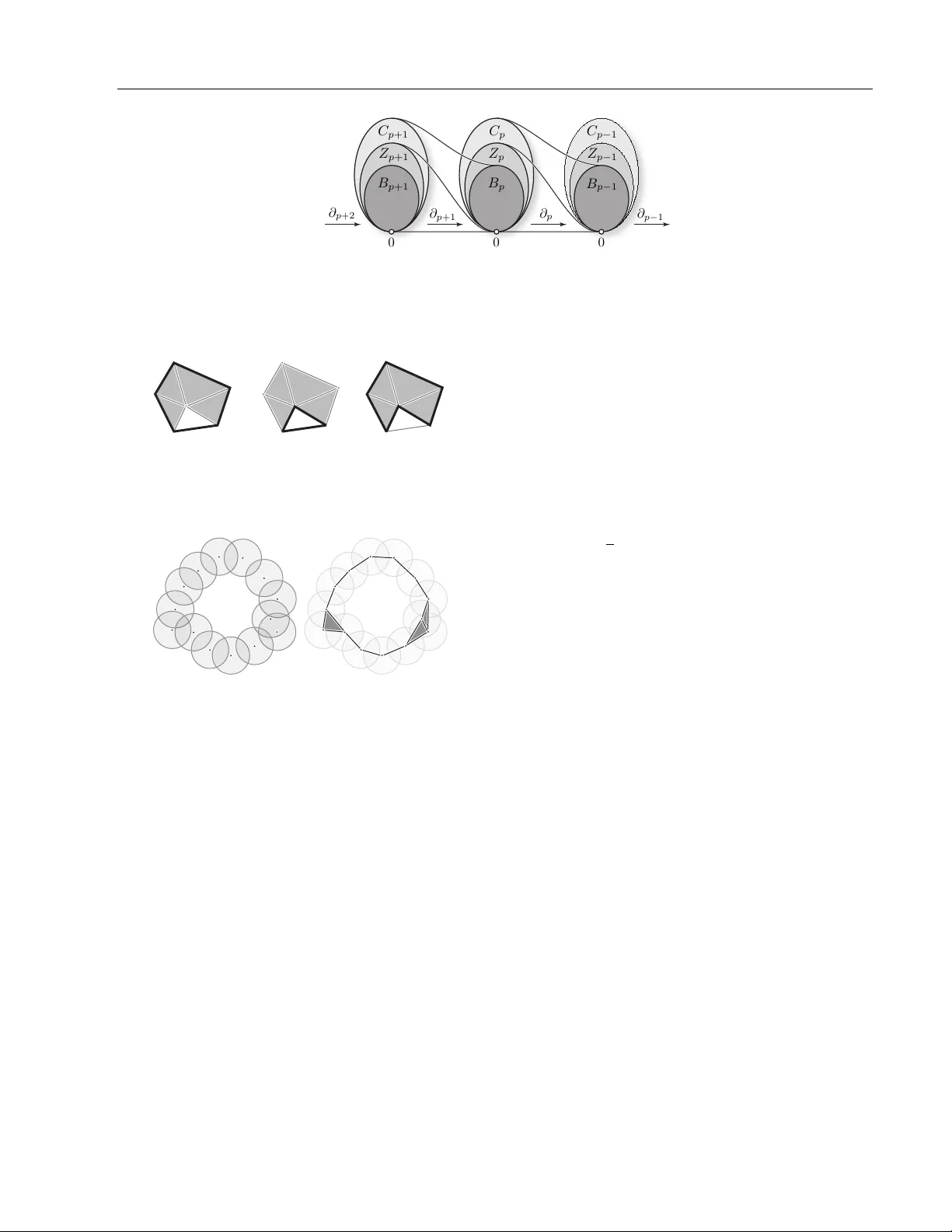
Minimax Rates for Homology Inference Siv araman Balakrishnan † Alessandro Rinaldo † Don Sheeh y †† Aarti Singh † Larry W asserman † † Carnegie Mellon Univ ersity †† INRIA Abstract Often, high dimensional data lie close to a lo w-dimensional submanifold and it is of in- terest to understand the geometry of these submanifolds. The homology groups of a manifold are imp ortan t top ological inv ariants that pro vide an algebraic summary of the manifold. These groups con tain rich top o- logical information, for instance, ab out the connected comp onen ts, holes, tunnels and sometimes the dimension of the manifold. In this pap er, w e consider the statistical prob- lem of estimating the homology of a mani- fold from noisy samples under sev eral differ- en t noise mo dels. W e derive upp er and lo wer b ounds on the minimax risk for this problem. Our upper b ounds are based on estimators whic h are constructed from a union of balls of appropriate radius around carefully selected p oin ts. In eac h case w e establish complemen- tary lo wer b ounds using Le Cam’s lemma. 1 In tro duction Let M be a d -dimensional manifold em b edded in R D where d ≤ D . The homolo gy gr oups H ( M ) of M [11] is an algebraic summary of the properties of M . The homology groups of a manifold describ e its top ologi- cal features such as its connected components, holes, tunnels, etc. In machine learning, there is muc h fo cus on cluster- ing. Ho wev er, the clusters are only the zeroth order homology and hence only scratch the surface of the top ological information in a dataset. Extracting in- formation beyond clustering is kno wn as top ological data analysis. It is worth emphasizing that the ho- mology groups are top ological in v ariants of a manifold App earing in Proceedings of the 15 th In ternational Con- ference on Artificial Intelligence and Statistics (AIST A TS) 2012, La Palma, Canary Islands. V olume XX of JMLR: W&CP XX. Copyrigh t 2012 by the authors. that can be efficiently computed [4, 5]. Examples of applications of homology inference hav e b een growing rapidly in the last few years. Homology inference has found application in medical imaging and neuroscience [3, 21], sensor netw orks [6, 20], landmark-based shap e data analyses [10], proteomics [19], microarra y analysis [7] and cellular biology [14]. The b o oks b y [8, 18, 23] con tain v arious case studies in applications in fields ranging from computational biology to geoph ysics. In this pap er we study the problem of estimating the homology of a manifold M from a noisy sample Y 1 , . . . , Y n . Sp ecifically , w e b ound the minimax risk R n ≡ inf b H sup Q ∈Q Q n  b H 6 = H ( M )  (1) where the infimum is ov er al l estimators b H of the ho- mology of M and the supremum is o ver appropriately defined classes of distributions Q for Y . Note that 0 ≤ R n ≤ 1 with R n = 1 meaning that the problem is hopeless. Bounding the minimax risk is equiv alent to bounding the sample c omplexity of the best p ossible estimator, defined b y n (  ) = min  n : R n ≤   where 0 <  < 1. 1.1 Related W ork Other w ork on statistical homology includes that of Chazal et. al. [2] who sho w under certain conditions the homology estimate of a manifold from a sample is stable under noise p erturbation that is small in a W asserstein sense. Kahle [13] studies the homology of random geometric graphs and pro ves man y threshold and cen tral limit theorems for their homology . Adler et. al. [1] study the homology induced b y the level sets of certain Gaussian random fields. There is also a large literature on manifold denoising that fo cuses on asp ects of the manifold not related to homology; see for instance [12] and references therein. Our upp er bounds mainly generalize those in the work of Niyogi, Smale and W einberger (henceforth NSW) [16, 17]. They establish a general result showing that when al l the samples are dense in a thin region sur- Minimax Rates for Homology Inference rounding the manifold, a union of appropriately sized balls around the samples can be used to construct an accurate estimate of the homology with high probabil- it y . Under a v ariety of differen t noise mo dels we will sho w that even when al l the samples are not close to the manifold it is possible to “clean” the samples (es- sen tially removing those in regions of lo w-densit y) and b e left with samples whic h are dense in a thin region around the manifold. In the case of additive noise with general noise dis- tributions ho w ev er, we cannot exp ect to o man y sam- ples to fall close to the manifold. W e will sho w that when the noise distribution is known one can use a statistical deconv olution pro cedure to obtain a “de- con volv ed measure” concen trated around the manifold from whic h we can in turn draw a small n um b er of samples and apply the cleaning pro cedure describ ed ab o ve to them. Decon volution has b een extensiv ely studied in the statistical literature (see [9] and refer- ences therein). Most related to our application is the w ork of Koltchinskii [15] who uses deconv olution to estimate the dimension and cluster tree of a distribu- tion supp orted on a submanifold. W e defer a detailed comparison to Section 5.4.1 after the necessary prelim- inaries ha ve b een introduced. T o the b est of our knowledge, ours is the first pap er to obtain low er and upp er minimax b ounds for the prob- lem of inferring the homology of a manifold. There are a few existing results on upper bounds. A summary of previous results and the results in this pap er are in T able 1. Outline. In Section 2 w e describ e the statistical mo del. In Section 3 w e giv e a brief description of homology . In Section 4 w e giv e an o verview of our techniques. W e deriv e the minimax rates for the four noise settings in Section 5. T echnical pro ofs are contained in the App endix. 2 Statistical Mo del W e assume that the sample { Y 1 , . . . , Y n } ⊂ R D con- stitutes a set of “noisy” observ ations of an unknown d -dimensional manifold M , with d < D , whose ho- mology we seek to estimate. The distribution of the sample depends on the prop erties of the manifold M as well as on the type of sampling noise, whic h we de- scrib e b elow by formulating v arious statistical mo dels for sampling data from manifolds. Notation. W e let B k r ( x ) denote a k -dimensional ball of radius r centered at x . When k = D , w e write B r ( x ) instead of B D r ( x ). F or any set M and any σ > 0 define tub e σ ( M ) = S x ∈ M B σ ( x ). Let v k denote the volume of the k -dimensional unit ball. Finally , for clarity we let c 1 , c 2 , . . . , C 1 , C 2 , . . . denote v arious p ositive con- stan ts whose v alue can b e different in different expres- sions. The constants will be sp ecified in the corre- sp onding pro ofs. Manifold Assumptions. W e assume that the un- kno wn manifold M is a d -dimensional smooth compact Riemannian manifold without b oundary em b edded in the compact set X = [0 , 1] D . W e further assume that the volume of the manifold is b ounded from abov e b y a constan t whic h can dep end on the dimensions d, D , i.e. w e assume v ol( M ) ≤ C D,d . Compact d -dimensional manifolds without boundary typically reside in an am- bien t dimension D > d , an assumption we will mak e throughout this pap er. The main regularit y condition w e imp ose on M is that its c ondition numb er b e not to o small. The c ondition numb er κ ( M ) (see [16]) is the largest n umber τ such that the open normal bundle ab out M of radius r is im b edded in R D for ev ery r < τ . F or τ > 0 let M ≡ M ( τ )= n M : κ ( M ) ≥ τ o denote the set of all such manifolds with condition n um b er no smaller than τ . A manifold with large condition n um- b er do es not come to o close to b eing self-intersecting. W e consider the collection P ≡ P ( M ) ≡ P ( M , a ) of all probability distributions supp orted ov er manifolds M in M having densities p with resp ect to the volume form on M uniformly b ounded from b elo w b y a con- stan t a > 0, i.e. 0 < a ≤ p ( x ) < ∞ for all x ∈ M . F or exp ositional clarity we treat a as a fixe d constant although our upp er and low er b ounds match in their dep endence on a . The Noise Mo dels. W e consider four noise mo dels and, for each of them, w e sp ecify a class Q of proba- bilit y distributions for the sample. Noiseless. W e observe data Y 1 , . . . , Y n ∼ P where P ∈ P . In this case, Q = Q ( τ ) = P . Clutter Noise. W e observ e data Y 1 , . . . , Y n from the mixture Q = (1 − π ) U + π P where, P ∈ P , 0 ≤ π ≤ 1 and U is a uniform distribution on X . The p oints dra wn from U are called bac kground clutter. Then Q = Q ( π , τ ) = n Q = (1 − π ) U + π P : P ∈ P o . Notice that π = 1 reduces to the noiseless case. T ubular Noise. W e observe Y 1 , . . . , Y n ∼ Q M ,σ where Q M ,σ is uniform on a tub e of size σ around M . In this case Q = Q ( σ, τ ) = n Q M ,σ : M ∈ M o . A dditive Noise. The data are of the form Y i = X i +  i , where X 1 , . . . , X n ∼ P , for some P ∈ P , and  1 , . . . ,  n are a sample from a noise distribution Φ. Note that Q = P ? Φ, that is, Q is the conv olution of P and Φ. W e consider tw o cases: 1. Φ is a D -dimensional Gaussian with mean Balakrishnan, Rinaldo, Sheehy , Singh, W asserman Noise Mo del Noiseless Clutter T ubular Additiv e Gaussian General additiv e ( τ fixed) Upp er Bound NSW This pap er NSW This pap er This pap er Lo w er Bound This pap er This pap er This pap er This pap er This pap er T able 1: Summary of our contributions (0 , . . . , 0) and co v ariance σ 2 I , with σ  τ . Define Q = Q ( σ, τ ) = n Q = P ? Φ : P ∈ P o . 2. Φ is any known noise distribution whose F ourier transform is b ounded a w ay from 0 but with the added restriction that we only consider manifolds with τ being a fixed constant. Then Q = Q (Φ) = n Q = P ? Φ : P ∈ P τ o . where P τ is the subset of P comprised of distributions supported on man- ifolds M with condition num b er at least as large as the fixe d v alue τ . The noise model used in [17] is to tak e the noise at an y p oin t to b e only along the normal fibres; this seems unnatural and w e will not consider that mo del here. In almost all of the distribution classes considered we allo w for τ to v anish as n gets bigger, which is equiv- alen t to letting the difficulty of the statistical problem increase with the sample size. T o this end, we will also analyze the quan tity τ n ≡ τ n (  ) = inf { τ : R n ≤  } , whic h corresp onds to the smallest condition n umber that p ermits accurate estimation. W e call this the r esolution . 3 Homology Often in our pap er we will use phrases lik e “the homol- ogy of the union of balls around samples”. In this sec- tion we explain this usage and discuss briefly simplicial homolo gy (see Hatcher (2001) for a detailed treatmen t) and its computation. The homology H of a space S is a collection of groups that corresp ond to top ological features of S . In what follo ws, it might help the reader’s intuition to imagine that w e are starting with a dense sample of p oin ts U on a manifold and building a collection of simplices from these points. The union of balls S y ∈ U B  ( y ) giv es a geometric appro ximation to the underlying manifold. This is how ev er a con tin uous (infinite) collection of p oin ts. T o make computation tractable w e need to b e able to reduce the computation of homology from a con tinuous space to its discretization. The ˇ Cec h com- plex (a particular simplicial c omplex , see Figure 3) whic h is described b elow gives a discrete representa- tion of the union of balls. A classic result in top ology called the Nerve Theorem [11] states that the homol- ogy of S y ∈ U B  ( y ) is identical to the homology of the corresp onding ˇ Cec h complex. W e now describ e a simplicial complex and its homol- ogy . A simplicial c omplex is a hereditary set system K o ver a vertex set V , i.e. σ ⊂ σ 0 ∈ K implies that σ ∈ K . The dimension of a simplex σ is | σ | − 1; singletons are 0-simplices or vertices, pairs in K are 1-simplices or edges, triples are 2-simplices or triangles, etc. A p - c hain is a formal sum of p -simplices. The co efficien ts are taken in Z 2 , the integers mo d 2. 1 Th us, c hains ma y b e viewed as subsets of simplices and addition (mod 2) as symmetric difference of sets. Addition of c hains forms an ab elian group called the chain gr oup C p with 0 denoting the empt y chain. A p -simplex σ = { v 0 , . . . , v p } has p + 1 simplices of di- mension p − 1 on its b oundary , denoted σ i = σ \ { v i } . The b oundary of a simplex is ∂ p σ = P p i =0 σ i . The b oundary op er ator ∂ p : C p → C p − 1 is the natural ex- tension of the b oundary of a simplex to the b oundary of a c hain: ∂ p c = P σ ∈ c ∂ p σ . The kernel and image of the boundary op erator are t wo important subgroups of the chain group: the cycle gr oup : Z p = ker ∂ p = { z ∈ C p : ∂ p z = 0 } , and the b oundary gr oup : B p = im ∂ p = { ∂ p +1 c : c ∈ C p +1 } . The cycles Z p are those chains that ha ve b oundary 0. The b oundary cycles B p are those p -c hains that are the b oundary of some p + 1-c hain. It is easy to c heck that ∂ p − 1 ∂ p c = 0 and th us B p ⊂ Z p ⊂ C p . See Figure 1. Tw o cycles z 1 , z 2 ∈ Z p are homolo gous if z 1 − z 2 ∈ B p , i.e. their difference is the b oundary of a p + 1-c hain. The p th homology group H p is defined as the quo- tien t group Z p /B p . That is, the homology group is a collection of equiv alence classes of cycles. The first homology group H 0 corresp onds to connected comp o- nen ts (clusters). The next homology group H 1 corre- sp onds to cycles (or lo ops). Higher order homology groups corresp ond to equiv alence classes of higher di- mensional cycles. 2 The homology of K is the collection H of all its homology groups. The ˇ Cec h complex is a sp ecific simplicial complex de- fined as follows. Fix some  > 0 and a set of p oints S ⊂ R D . The ˇ Ce ch c omplex consists of all simplices σ suc h that T x ∈ σ B  ( x ) 6 = ∅ where B  ( x ) is a ball of radius  cen tered at x . See Figure 3. 1 In general, homology ma y be defined o ver an y ring, but w e stick with Z 2 for ease of exp osition and computation. 2 In tuitively , b oundary cycles are “filled in” cycles and t wo cycles are homologous if one cycle can b e deformed in to the other cycle. Minimax Rates for Homology Inference ∂ p +1 ∂ p ∂ p − 1 0 0 0 C p +1 C p C p − 1 Z p − 1 Z p Z p +1 B p +1 B p − 1 B p ∂ p +2 Figure 1: Relationship b etw een chains C p , cycles Z p = ker ∂ p and b oundaries B p = im ∂ p +1 . The chains C p are just collections of simplices. The chains in Z p are the cycles. The cycles in B p are the cycles that happ en to b e b oundaries of c hains in C p +1 . + = Figure 2: The sum of t wo 1-cycles is another 1-cycle. Here the cycles are homologous b ecause their sum (in Z 2 )is the b oundary of a 2-c hain of triangles. Figure 3: A union of balls and its corresponding ˇ Cec h complex. Since the coefficient ring is a field, the computations ma y be completely describ ed b y linear algebra. The groups C p , Z p , B p , and H p are vector spaces and the b oundary op erators are linear maps. It is p ossible to efficien tly compute the homology groups of a simplicial complex in time polynomial in the size of the complex. The algorithm only in volv es row reduction on the ma- trix represen tations of ∂ p . 4 T ec hniques 4.1 T echniques for low er b ounds The total variation distanc e b etw een tw o measures P and Q is defined by TV ( P , Q ) = sup A | P ( A ) − Q ( A ) | where the supremum is ov er all measurable sets. It can b e shown that TV ( P , Q ) = P ( G ) − Q ( G ) = 1 − R min( P , Q ) where G = { y : p ( y ) ≥ q ( y ) } and p and q are the densities of P and Q with resp ect to an y measure µ that dominates b oth P and Q . W e shall make rep eated use of Le Cam’s lemma which w e now state (see, e.g., [22]). Lemma 1 ( Le Cam). L et Q b e a set of distributions. L et θ ( Q ) take values in a metric sp ac e with metric ρ . L et Q 1 , Q 2 ∈ Q b e any p air of distributions in Q . L et Y 1 , . . . , Y n b e dr awn iid fr om some Q ∈ Q and denote the c orr esp onding pr o duct me asur e by Q n . Then inf b θ sup Q ∈Q E Q n h ρ ( b θ , θ ( Q )) i ≥ 1 8 ρ ( θ ( Q 1 ) , θ ( Q 2 )) (1 − TV ( Q 1 , Q 2 )) 2 n wher e the infimum is over al l estimators. Le Cam’s lemma makes precise the intuition that if there are distinct mem b ers of the class Q for whic h the data generating distributions are close then the statistical problem is hard giv en a small sample. When w e apply Le Cam’s lemma in this pap er, Q 1 and Q 2 will b e asso ciated with tw o different manifolds M 1 and M 2 . W e will take θ ( Q ) to b e the homology of the manifold and ρ ( θ ( Q 1 ) , θ ( Q 2 )) = 1 if the homolo- gies are the different and ρ ( θ ( Q 1 ) , θ ( Q 2 )) = 0 if the homologies are the same. The subtlety of establishing tight lo wer b ounds b oils down to the task of finding a set of distributions in the class Q for whic h the homol- ogy of the underlying submanifolds are distinct but whose empirical distributions are hard to distinguish from a small n umber of samples. W e will use tw o representativ e manifolds M 1 and M 2 in the application of LeCam’s lemma which we de- scrib e here. See Figure 4. The manifold M 1 is a pair of 1 − τ d -balls (sho wn in blue) em b edded 2 τ apart in R D joined smo othly at their ends (shown in red). The manifold M 2 is a pair of d -annuli (shown in blue) em b edded 2 τ apart with outer radius 1 − τ and inner radius 4 τ , smoothly joined at both the inner and outer ends (shown in red). It is clear from the construction that b oth these manifolds are d-dimensional compact, ha ve no b oundary and hav e condition n umber τ . It is also the case that H ( M 1 ) 6 = H ( M 2 ). If there exist t wo manifolds M 1 and M 2 with corre- Balakrishnan, Rinaldo, Sheehy , Singh, W asserman Figure 4: The tw o manifolds M 1 and M 2 , with d = 1, D = 2 sp onding distributions Q 1 and Q 2 in Q such that (i) H ( M 1 ) 6 = H ( M 2 ) and (ii) Q 1 = Q 2 then we say that the mo del Q is non-identifiable . In this case, reco ver- ing the homology is imp ossible and we write R n = 1 and n (  ) = ∞ . 4.2 T echniques for upp er b ounds T o establish an upp er b ound we need to construct an estimator that achiev es the upper bound. In the noise- less and tubular noise cases the samples are in a thin region around the manifold and our estimator is con- structed from a union of balls (of a carefully c hosen radius) around the sample p oin ts. In the case of clutter noise and additiv e Gaussian noise samples are concentrated around the manifold but a few samples may b e quite far aw a y from the manifold. In these cases our upp er b ounds are obtained by an- alyzing the p erformance of the Algorithm 1 ( CLEAN ) with a carefully sp ecified threshold and radius, which is used to remov e p oints in regions of low densit y far a wa y from the manifold. Our estimator is then con- structed from a union of balls around the remaining p oin ts. In the case of additiv e noise with general Algorithm 1 CLEAN • IN: ( X i ) n i =1 , threshold t , radius r 1. Construct a graph G r with no des { X i } n i =1 . In- clude edge ( X i , X j ), if || X i − X j || ≤ r . 2. Mark all vertices with degree d i ≤ ( n − 1) t . • OUT: All unmarked vertices kno wn distribution the samples are not exp ected to b e concentrated around the manifold. W e will first use deconv olution to estimate a deconv olv ed measure b P n whic h w e will sho w is densely concen trated in a thin region around the manifold. W e will then dra w samples from this measure, clean them and construct a union of balls of appropriate radius around the re- maining samples, and show that this set has the right homology with high probabilit y . W e now briefly review statistical decon v olution. W e refer the interested reader to the work of F an [9] for more details and to [15] for an application related to ours. The pro cedure is similar to kernel density esti- mation with a kernel mo dified to account for the ad- ditiv e noise. F or symmetric noise distributions Φ, we consider tw o kernels K and Ψ such that K ? Φ = Ψ, where ? denotes con v olution. The deconv olution es- timator is b P n ( A ) = 1 /n P n i =1 K ( Y i − A ). It is easy to verify that E b P n = P ? Ψ similar to regular k ernel densit y estimation with the kernel Ψ. In the noiseless case we can ev en take K = Ψ = δ 0 (a Dirac at 0) and get bac k the empirical distribution of the sample. More generally , we will b e interested in Ψ that satis- fies Ψ { x : | x | ≥  } ≤ γ . for  and γ that we will later sp ecify . In each of the ab ov e cases our final estimator is con- structed from a union of balls around appropriate p oin ts, and our theorems will sho w that these hav e the correct homology with high probabilit y . T o compute the homology one would construct the corresp onding ˇ Cec h complex and compute its “boundary matrices” (as describ ed in Section 3). Recov ering the homology from these matrices consists of linear algebraic manip- ulation. There are several fast algorithms to compute the homology (either exactly [4] or approximately [5]) of the ˇ Cec h complexes from large point sets in high dimensions. 5 Minimax Rates W e no w deriv e the minimax rates for homology esti- mation under the four noise mo dels describ ed in sec- tion 2. There are three quantities of in terest: the minimax risk R n , the resolution τ n and the sample complexit y n (  ). W e write R n  a n (similarly for τ n  a n ) if there are p ositive constants c and C suc h that c ≤ R n /a n ≤ C for all large n . Similarly , w e write n (  )  a (  ) if there are positive constan ts c and C suc h that c ≤ n (  ) /a (  ) ≤ C for all small  . Our analysis will show that the rates (as a function of n ) are t ypi- cally polynomial for the resolution and exp onential for the risk. W e will often match upp er and low er b ounds on sample complexity and resolution only up to loga- rithmic factors, and corresp ondingly those on the risk upto p olynomial factors. In this case we will use the notation R n  ∗ a n , τ n  ∗ a n , and n (  )  ∗ a (  ). It is worth emphasizing at this p oint that despite the fact that we use t w o sp ecific manifolds in the appli- cation of Le Cam’s lemma, the resulting low er b ound Minimax Rates for Homology Inference holds for al l manifolds in M and al l distributions in Q . Le Cam’s lemma allows one to get a low er b ound that holds for any estimator by using two carefully c hosen distributions in Q . The upper b ounds are from sp ecific estimators and they establish an upp er b ound on the num ber of samples to estimate the homology of an y manifold in our class. 5.1 Noiseless Case Theorem 1. F or al l τ ≤ τ 0 ( a, d ) , in the noiseless c ase the minimax r ate, R n  ∗ e − nτ d , wher e τ 0 ( a, d ) is a c onstant which dep ends on a and d . Also, n (  )  ∗ τ − d log(1 / ) and τ n  ∗ ((1 /n ) log(1 / )) 1 /d . W e provide pro of sketc hes for the low er and upper b ounds on R n separately . Lo w er Bound: Pro of Sketc h T o obtain a lo wer b ound on the minimax risk o ver the class Q ( τ ) w e will consider the t w o carefully c hosen manifolds M 1 and M 2 describ ed earlier. W e further need to sp ecify the density on each of the manifolds, and w e choose t wo densities from P so that the data distributions are as similar as p ossible while resp ecting the constraint p ( x ) ≥ a . The construction is describ ed in more detail in the App endix A.1.1, but for now it suffices to notice that the t wo densities can b e constructed to differ only on the sets W 1 = M 1 \ M 2 and W 2 = M 2 \ M 1 and can b e made as low as a on one of these sets. A straigh tforward calculation sho ws that TV ( p 1 , p 2 ) ≤ a max(v ol( W 1 ) , v ol( W 2 )) ≤ C d aτ d where the constant C d dep ends on d . Now, we apply Le Cam’s lemma to obtain that R n ≥ 1 8  1 − C d aτ d  n ≥ 1 8 e − 2 C d naτ d for all τ ≤ τ 0 ( a, d ). τ 0 ( a, d ) is a constan t depending on a and d . The low er b ound of Theorem 1 follo ws. Upp er Bound: Pro of Sketc h In the noiseless case the samples are densely concen- trated around the manifold and our estimator is con- structed from a union of balls of radius τ / 2 around the sample p oin ts. The upp er b ound on the mini- max risk follo ws from a straigh tforward mo dification of the results of [16]. F or completeness, we repro duce an adaptation of their main homology inference theo- rem (Theorem 3.1) here. Lemma 2. [NSW] L et 0 <  < τ and let U = S n i =1 B  ( X i ) . L et b H = H ( U ) . L et ζ 1 = vol ( M ) a cos d θ 1 vol ( B d / 4 ) , ζ 2 = vol ( M ) a cos d θ 2 vol ( B d / 8 ) , θ 1 = sin − 1  8 τ and θ 2 = sin − 1  16 τ . Then for al l n > ζ 1  log( ζ 2 ) + log  1 δ  , P ( b H 6 = H ( M )) < δ . By assumption vol ( M ) ≤ C D,d for some constan t C D,d dep ending on d and D . T o obtain a sample complex- it y b ound w e simply c hoose  = τ / 2 and this giv es us n (  ) ≤ C 1 / ( aτ d )( C 2 log(1 / ( aτ d )) + log(1 / )) which matc hes the low er b ound upto the factor of log(1 /τ ). F urther calculation (see App endix A.1.1) then sho ws that as desired R n ≤ C 1 /τ d exp( − C 2 naτ d ) for appro- priate constants C 1 , C 2 , and τ n ≤ C ( log n log(1 / ) an ) 1 /d . This establishes Theorem 1. 5.2 Clutter Noise Theorem 2. F or al l τ ≤ τ 0 ( a, d ) , in the clutter noise c ase, R n  ∗ e − nπ τ d , wher e τ 0 ( a, d ) is a c onstant which dep ends on a and d . Also, n (  )  ∗ (1 / ( π τ d ) log(1 / ) and τ n  ∗ (1 / ( nπ ) log(1 / )) 1 /d . Lo w er Bound: Pro of Sketc h The low er b ound for the class Q ( π , τ ) follows via the same construction as in the noiseless case. In the cal- culation of the total v ariation distance (see App endix A.1.2) w e hav e instead TV ( q 1 , q 2 ) ≤ π a max(vol( W 1 ) , v ol( W 2 )) ≤ C d π aτ d where C d dep ends on d . As before the low er bound follo ws from the application of Le Cam’s lemma. Upp er Bound: Pro of Sketc h As a preliminary step we clean the data samples to eliminate p oints that are far aw ay from, while retaining those close to, the manifold. Our analysis shows that Algorithm 1 will ac hiev e this, with high probabilit y for a carefully c hosen threshold and radius. W e then sho w that taking a union of balls of the appropriate radius around the remaining p oin ts will give us the correct homology , with high probability . W e give an outline here and defer details to App endix A.1.2. 1. W e define tw o regions A = tub e r ( M ) and B = R D \ tub e 2 r ( M ) where r < ( √ 9 − √ 8) τ 2 . 2. W e then inv ok e Algorithm CLEAN on the data with threshold t =  v D s D (1 − π ) vol(Bo x) + π av d r d cos d θ 2  and radius 2 r . Let I b e the set of v ertices re- turned. 3. Through careful analysis we show that with high probabilit y I con tains al l the v ertices from the region A and none of the p oints in region B . 4. W e further show that the retained p oints form a thin dense co ver of the manifold M , i.e. n M ⊂ S i ∈ I B 2 r ( X i ) o . Balakrishnan, Rinaldo, Sheehy , Singh, W asserman 5. Using a straightforw ard corollary of Lemma 2 we sho w that this thin dense cov er can be used to reco ver the homology of M with high probability . F ormally , in App endix A.1.2 we prov e the following lemma, Lemma 3. If n > max( N 1 , N 2 ) , and r < ( √ 9 − √ 8) τ 2 wher e N 1 = 4 κ log( κ ) with κ = max  1 + 200 3 ζ log  2 δ  , 4  and N 2 = 1 ζ  log  v ol( M ) cos d ( θ ) v d r d  + log  2 δ  wher e ζ = π av d r d cos d ( θ ) and θ = sin − 1 ( r / 2 τ ) , then after cle aning the p oints { X i : i ∈ I } ar e al l in tub e 2 r ( M ) and ar e 2 r dense in M . L et U = S i ∈ I B w ( X i ) with w = r + τ 2 and let b H = H ( U ) . We have that b H = H ( M ) with pr ob ability at le ast 1 − δ . T aking r = ( √ 9 − √ 8) τ / 4, w e obtain the sample complexit y b ound, n (  ) ≤ C 1 π τ d (log C 2 τ d + log( C 3 / )). Giv en this sample complexity upper b ound, the upp er b ounds on minimax risk and resolution follo w iden tical argumen ts to the noiseless case (App endix A.1.1). 5.3 T ubular Noise Under this noise mo del we get samples uniformly from a tubular region of width σ around the manifold. This mo del highlights an important phenomenon in high- dimensions. Although, we receive samples uniformly from a full D dimensional shap e these samples con- cen trate tightly around a d dimensional manifold. W e sho w that with some care we can still reconstruct the homology at a rate indep enden t of D . Theorem 3. Under the tubular noise mo del we estab- lish the fol lowing c ases. 1. If σ ≥ 2 τ then the mo del is non-identifiable and henc e, R n = 1 and n (  ) > ∞ . 2. If σ ≤ C 0 τ , with C 0 smal l and τ ≤ τ 0 ( a, d ) , then R n  ∗ e − nτ d , wher e τ 0 ( a, d ) is a c onstant which dep ends on a and d . Also, n (  )  ∗ 1 /τ d and τ n  ∗ ( 1 n log(1 / )) 1 /d . Remark 1. The c ase when σ is very close to τ is signific antly mor e involve d sinc e it involves the exact c alculation of the volume of the tubular r e gion and es- tablishing tight upp er and lower b ounds her e is an op en pr oblem we ar e attempting to addr ess in curr ent work. Lo w er b ound: Pro of Sketc h 1. When d < D and σ ≥ 2 τ the tw o manifolds M 1 and M 2 that we hav e considered thus far are still iden tifiable b ecause ev en when σ ≥ τ M 2 has a “dimple” along the co-dimensions that M 1 do es not. T o show that the class Q is still not iden- tifiable we require a different construction. Con- sider the manifolds M 1 and M 2 with tw o p oints placed abov e and below the manifold at a dis- tance 2 τ ab o ve their centers along each of the co- dimensions. Denote these new manifolds M 0 1 and M 0 2 . It is clear that H ( M 0 1 ) 6 = H ( M 0 2 ), ho w ever Q 0 1 = Q 0 2 since the extra p oin ts hide the “dimple” and the t wo manifolds cannot b e distinguished. 2. When d < D , and σ ≤ C 0 τ we return to our old constructions of M 1 and M 2 . There is how- ev er an imp ortant difference in that the tw o man- ifolds differ on full D -dimensional sets, and one migh t susp ect that T V ( q 1 , q 2 ) = O ( τ D ) or per- haps O ( σ D − d τ d ). As we show in App endix A.1.3 ho wev er, T V ( q 1 , q 2 ) is still O ( τ d ), and we recov er an iden tical low er b ound to the noiseless case. Upp er b ound: Pro of Sketc h W e are interested in case when σ ≤ C 0 τ (in particular σ < τ / 24 will suffice). Our proof will in volv e t wo main steps whic h we sketc h here. 1. W e first show that if w e consider balls of suffi- cien tly large radius  (compared to σ ) then the probabilit y mass in these balls is O (  d ). This is a manifestation of the phenomenon alluded to earlier: inside large enough balls the mass is concen trated around the low er dimensional man- ifold. Precisely , define k  = inf p ∈ M Q ( B  ( p )). In Lemma 9 in the App endix, we sho w that, if   σ is large, k  is of order Ω(  d ). 2. There is ho w ever a disadv antage to considering balls that are too large. The homology of the union of balls around the samples may no longer ha ve the right homology . Using to ols from NSW, w e show in the App endix that we can balance these tw o considerations for manifolds with high condition num b er, i.e. provided σ < τ / 24, we can c ho ose balls that are b oth large relative to σ and whose union still has the correct homology . W e will prov e the following main lemma in the Ap- p endix. Lemma 4. L et N  b e the  -c overing numb er of the submanifold M . L et U = S n i =1 B  + τ / 2 ( X i ) . L et b H = H ( U ) . Then if n > 1 k  (log( N  ) + log(1 /δ )) , P ( b H 6 = H ( M )) < δ as long as σ ≤ / 2 and  < ( √ 9 − √ 8) τ 2 . Notice, that we require σ < ( √ 9 − √ 8) τ 4 whic h is satisfied if σ < τ / 24 (for instance). T o obtain the upp er b ound set  = 2 σ , and observe that N  = O (1 / d ) = O (1 /τ d ) Minimax Rates for Homology Inference and k  = O (  d ) = O ( τ d ). This giv es us that if n ≥ C 1 τ d (log( C 2 τ d ) + log( 1 δ )) w e recov er the right homol- ogy with probability at least 1 − δ . The upp er b ound on minimax risk and resolution follows from similar argumen ts to those made previously . 5.4 Additive Noise F or additive noise we consider tw o cases. In the first case, we derive the minimax rates for additiv e Gaus- sian noise under the somewhat restrictive assumption that C √ D σ < τ . This problem is related of the prob- lem of separating mixtures of Gaussians (which corre- sp onds to the case where the manifold is a collection of p oints and 2 τ is the distance betw een the closest pair). In this case hav e the follo wing theorem. Theorem 4. F or al l τ ≤ τ 0 ( a, d ) and 8 √ D σ < τ , R n  ∗ e − nτ d , wher e τ 0 ( a, d ) is a c onstant which de- p ends on a and d . Also, n (  )  ∗ (1 /τ d ) log(1 / ) and τ n  ∗ ((1 /n ) log(1 / )) 1 /d . As in the clutter noise case we need to first clean the data and then take a union of balls around the p oints whic h survive. W e analyze this pro cedure in the Ap- p endix. 5.4.1 Deconv olution Here we consider more general known noise distribu- tions but w ork ov er the class of distributions Q (Φ) o ver manifolds with τ fixed. W e first use decon volution to estimate a decon volv ed measure b P n whic h is concen- trated around the manifold. W e then dra w samples from this measure, clean them and construct a union of balls H around these samples, and sho w that H has the right homology with high probability . The class of noise distributions we will consider satisfy the follow- ing assumption on its densit y . Assumption 1. Denote ρ ( R ) = inf | t | ∞ ≤ R | Φ ? ( t ) | , wher e R > 0 , | t | ∞ = max 1 ≤ j ≤ m | t j | and Φ ? ( t ) is the F ourier tr ansform of the symmetric noise density Φ . We assume ρ ( R ) > 0 . This is a standard assumption in the literature on de- con volution (see [9, 15]), since as describ ed deconv o- lution requires us to divide b y the F ourier transform of the noise which needs to b e b ounded aw a y from 0 for the procedure to b e w ell b ehav ed. The assump- tion is satisfied by a v ariety of noise distributions in- cluding Gaussian noise. Our main result says that for this broad class of noise distributions the decon volu- tion procedure described abov e will achiev e an optimal rate of con vergence. Theorem 5. In the additive noise c ase with τ fixe d for Φ satisfying Assumption 1. R n  e − n . Henc e, n (  )  log(1 / ) . Lo w er Bound: Pro of Sk etch T o obtain the low er b ound one can consider the same construction from the previous subsection with additive Gaussian noise. If τ is taken to b e fixed we obtain the desired b ound. Upp er Bound: Pro of Sketc h Our pro of of the up- p er b ound follows similar lines to that of Koltchinskii [15]. W e deviate in tw o significant asp ects. Koltc hin- skii only assumes an upp er b ound on the densit y , whic h he shows is sufficient to estimate weak geomet- ric characteristics like the dimension of the manifold. T o show that we can accurately reconstruct its homol- ogy we require b oth an upp er and low er b ound and our metho ds are quite differen t. Koltc hinskii uses an epsilon net of the entir e compact set containing the manifold critically in his construction and his proce- dure is th us not implementable/practical. Our algo- rithm instead draws a small num b er of samples from the deconv olved measure and uses those to estimate the homology resulting in a practical pro cedure. W e pro ve the following upp er b ound in the App endix. Lemma 5. Given n samples fr om Q (Φ) with Φ satis- fying Assumption 1, ther e exist C 1 , C 2 , c 1 > 0 such that P ( H ( H ) 6 = H ( M )) ≤ C 1 e − c 1 n , wher e H is a union of b al ls of r adius 5  + τ 2 c enter e d ar ound m ≥ C 2 n samples dr awn fr om the de c onvolve d me asur e b P n with a kernel Ψ with p ar ameters γ ,  (sp e cifie d in the pr o of ). The samples ar e cle ane d using the de c onvolve d me asur e by c onsidering b al ls of r adius 4  at a thr eshold 2 γ . Remark 2. The cle aning pr o c e dur e we use her e is dif- fer ent fr om the Algorithm CLEAN . We r emove p oints ar ound which a b al l of appr opriate r adius has low pr ob- ability mass under the de c onvolve d me asur e. This is e quivalent to using the de c onvolve d me asur e in plac e of the k-NN density estimate implicitly c onstructe d by the CLEAN pr o c e dur e. Simple calculations sho w that this lemma together with the low er bound give the exponential minimax rate describ ed in Theorem 5. 6 Conclusion W e hav e given the first minimax b ounds for homology inference. These b ounds give insight in to the intrinsic difficult y of the problem under v arious assumptions. Our b ounds sho w that it is often p ossible to estimate the homology of a manifold at fast rates indep endent of the am bient dimension. Actual implementation of homology inference has b e- come tractable thanks to adv ances in computational top ology . How ever, as our pro ofs reveal, recov ering the homology requires the careful selection of several tuning parameters. In current work, w e are develop- ing metho ds for c ho osing these parameters in a statis- tically sound, data-driv en wa y . Balakrishnan, Rinaldo, Sheehy , Singh, W asserman References [1] Rob ert J. Adler, Omer Bobrowski, Matthew S. Borman, Eliran Subag, and Shmuel W einberger. P ersistent homology for random fields and com- plexes. In James O. Berger, T on y Cai, and Iain M. Johnstone, editors, Borr owing Str ength: The ory Powering Applic ations - A F estschrift for L awr enc e D. Br own , pages 124–143. Institute of Mathematical Statistics, 2010. [2] F rederic Chazal, David Cohen-Steiner, and Quen tin Merigot. Geometric inference for prob- abilit y measures. F oundations of Computational Mathematics , 2011. to app ear. [3] Mo o K. Chung, P eter Bubenik, and Peter T. Kim. Persistence diagrams of cortical surface data. In Pr o c e e dings of the 21st International Confer enc e on Information Pr o c essing in Me dic al Imaging , IPMI ’09, pages 386–397, Berlin, Heidel- b erg, 2009. Springer-V erlag. [4] Vin de Silv a. PLEX: Simplicial c omplexes in MA TLAB . [5] Vin de Silv a and Gunnar Carlsson. T op olog- ical estimation using witness complexes. In M. Alexa and S. Rusinkiewicz, editors, Eur o- gr aphics Symp osium on Point-Base d Gr aphics . The Eurographics Asso ciation, 2004. [6] Vin de Silv a and Rob ert Ghrist. Cov erage in sen- sor net w orks via p ersistent homology . A lgebr aic & Ge ometric T op olo gy , 7:339–358, 2007. [7] Mary-Lee Dequean t, Sebastian Ahnert, Herb ert Edelsbrunner, Thomas M. A. Fink, Earl F. Glynn, Gay e Hattem, Andrzej Kudlicki, Y uriy Mileyk o, Jason Morton, Arcady R. Mushegian, Lior P ac h ter, Maga Rowic k a, Anne Shiu, Bernd Sturmfels, and Olivier P ourqui. Comparison of pattern detection methods in microarray time series of the segmen tation clo ck. PL oS ONE , 3(8):e2856, 08 2008. [8] H. Edelsbrunner and J.H. Harer. Computational top olo gy . American mathematical so ciety , 2009. [9] Jianqing F an. On the optimal rates of conv ergence for nonparametric deconv olution problems. Ann. Statist. , 19(3):1257–1272, 1991. [10] Jennifer Gamble and Giseon Heo. Exploring uses of persistent homology for statistical analysis of landmark-based shap e data. Journal of Multivari- ate Analysis , 101(9):2184–2199, Octob er 2010. [11] Allen Hatc her. Algebr aic T op olo gy . Cambridge Univ ersity Press, 2002. [12] Matthias Hein and Markus Maier. Manifold de- noising. In Bernhard Sch¨ olk opf, John C. Platt, and Thomas Hoffman, editors, NIPS , pages 561– 568. MIT Press, 2006. [13] Matthew Kahle. T op ology of random clique com- plexes. Discr ete Mathematics , 309(6):1658 – 1671, 2009. [14] P . M. Kasson, A. Zomoro dian, S. Park, N. Sing- hal, L. J. Guibas, and V. S. Pande. P ersisten t v oids: a new structural metric for membrane fu- sion. Bioinformatics , 23(14):1753–1759, 2007. [15] V. I. Koltchinskii. Empirical geometry of mul- tiv ariate data: a decon v olution approach. Ann. Statist. , 28(2):591–629, 2000. [16] Partha Niyogi, S tephen Smale, and Shm uel W ein- b erger. Finding the homology of submanifolds with high confidence from random samples. Dis- cr ete & Computational Ge ometry , 39(1-3):419– 441, 2008. [17] Partha Niyogi, S tephen Smale, and Shm uel W ein- b erger. A top ological view of unsup ervised learn- ing and clustering. SIAM J. Comput. , 40(3):646– 663, 2011. [18] V alerio Pascucci, Xa vier T rico che, Hans Hagen, and Julien Tiern y . T op olo gic al metho ds in Data A nalysis and Visualization: The ory, Algorithms and Applic ations . Springer, 2001. [19] Ahmet Sacan, Ozgur Ozturk, Hak an F erhatos- manoglu, and Y usu W ang. Lfm-pro: a to ol for detecting significant lo cal structural sites in pro- teins. Bioinformatics , 23:709–716, F ebruary 2007. [20] Vin De Silv a and Rob ert Ghrist. Homological sen- sor net works. Notic es of the Americ an Mathemat- ic al So ciety , 54:2007, 2007. [21] Gurjeet Singh, F acundo Memoli, Tigran Ishkhano v, Guillermo Sapiro, Gunnar Carls- son, and Dario L. Ringach. T op ological analysis of p opulation activit y in visual cortex. J. Vis. , 8(8):1–18, 6 2008. [22] Bin Y u. Assouad, Fano, and Le Cam. In D. P ollard, E. T orgersen, and G. Y ang, editors, F estschrift for Lucien L e Cam , pages 423–435. Springer, 1997. [23] Afra Zomorodian. T op olo gy for Computing . Cam- bridge Univ ersity Press, 2005. Minimax Rates for Homology Inference A App endix – Supplementary Material A.1 Key technical lemmas from [16] W e will need tw o technical lemmas, which follow from [16]. Lemma 6 ( Ball v olume lemma , Lemma 5.3 in [16]) . L et p ∈ M . Now c onsider A = M ∩ B  ( p ) . Then v ol ( A ) ≥ (cos( θ )) d v ol ( B d  ( p )) wher e B d  ( p ) is the a d -dimensional b al l in the tangent sp ac e at p , θ = sin − 1  2 τ . Next, consider a collection of balls { B r ( p i ) } i =1 ,...,n cen tered around points p i on the manifold and such that M ⊂ ∪ l i =1 B r ( p i ). Lemma 7 ( Sampling lemma , Lemma 5.1 in [16]) . L et A i = B r ( p i ) b e a c ol le ction of sets such that ∪ l i =1 A i forms a minimal c over of M . If Q ( A i ) ≥ α , and n > 1 α  log l + log  2 δ  then w.p. at le ast 1 − δ / 2 , e ach A i c ontains at le ast one sample p oint, and M ⊂ ∪ n i =1 B 2 r ( x i ) . F urther we have that l ≤ vol( M ) cos d ( θ ) v d r d . A.1.1 Pro ofs for the noiseless case Lo w er b ound Here we describ e the densities on the t wo manifolds M 1 and M 2 . There are t wo sets of inter- est to us: W 1 = M 1 \ M 2 whic h corresp onds to the t w o “holes” of radius 4 τ in the annulus, and W 2 = M 2 \ M 1 whic h corresponds to the d -dimensional piece added to smo othly join the inner pieces of the t wo ann uli in M 2 . By construction, v ol( W 1 ) = 2 v d (4 τ ) d where v d is the v olume of the unit d -ball. vol( W 2 ) is somewhat tricky to calculate exactly due to the curv ature of W 2 but it is easy to see that vol( W 2 ) is also O ( τ d ) with the constan t dep ending on d . One of the densities is constructed in the following w ay , on the set of larger volume (b etw een W 1 and W 2 ) we set p ( x ) = a , and ev enly distribute the rest of the mass o ver the remaining p ortion of the manifold (we are guaran teed that the mass on the rest of the manifold is at least a since otherwise the constrain t p ( x ) ≥ a can nev er b e satisfied). The other density is constructed to b e equal (to the first density) outside the set on which the t wo mani- folds differ. The remaining mass is spread evenly on the set where they do differ. W e are again guaranteed that p ( x ) ≥ a b y construction. Let us now calculate the TV b etw een these tw o den- sities. This is just the integral of the difference of the densities o v er the set where one of the densities is larger. Since the tw o densities are equal outside W 1 ∪ W 2 and disjoin t ov er W 1 ∪ W 2 it is clear that T V ( p 1 , p 2 ) = a max(v ol( W 1 ) , v ol( W 2 ) ≤ O ( aτ d ) with the constant dep ending on d . The lo w er b ound follo ws from the calculations in the main pap er. Upp er b ound The NSW lemma tells us that for n > ζ 1  log( ζ 2 ) + log  1 δ  , with ζ 1 = vol ( M ) a cos d θ 1 vol ( B d / 4 ) , ζ 2 = vol ( M ) cos d θ 2 vol ( B d / 8 ) , θ 1 = sin − 1  8 τ and θ 2 = sin − 1  16 τ , we ha ve P ( b H 6 = H ( M )) < δ . By assumption, w e hav e vol( M ) ≤ C . W e further tak e  = τ / 2. It is clear that in ζ 1 and ζ 2 all terms except the ball volumes are constant. This giv es us that ζ 1 = C 1 / ( aτ d ) and ζ 2 = C 2 / ( aτ d ). No w, the NSW lemma can b e restated as if n = C 1 /τ d (log( C 2 /τ d ) + log(1 /δ )) w e recov er the homol- ogy with probability at least 1 − δ . Notice that this means that the minimax risk ≤ δ . A straigh tforward rearrangement of this gives us R n ≤ C 2 / ( aτ d ) exp( − naτ d /C 1 ) for appropriate C 1 , C 2 . T o b ound the resolution w e rewrite this as R n ≤ exp  − naτ d C 1 + log  C 2 aτ d  One can v erify that if τ d ≤ C log n log (1 / ) n for an appropriately large C, we hav e R n ≤  as de- sired. A.1.2 Pro ofs for the clutter noise case Lo w er bound This is a straightforw ard extension of the noiseless case. The densities are constructed in an iden tical manner. The contribution to the densities from the clutter noise is identical in each case. As in the analysis for the noiseless case we b ound the total v ariation distance b etw een the tw o densities. W e hav e an additional factor of π whic h is the mixture weigh t of the comp onent corresp onding to the density on the manifold. T V ( q 1 , q 2 ) = π a max(vol( W 1 ) , v ol( W 2 )) ≤ C d π aτ d Giv en this b ound the calculations are iden tical to those in the noiseless case. Upp er b ound As a preliminary step we will need to clean the data to eliminate p oints that are far aw a y Balakrishnan, Rinaldo, Sheehy , Singh, W asserman from the manifold. Our analysis will sho w that Algo- rithm 1 will achiev e this, with high probability . W e will then show that taking a union of balls of the ap- propriate radius around the remaining p oints will give us the correct homology , with high probability . Let a = inf x ∈ M p ( x ), which is strictly p ositive by as- sumption. Define, A = tube r ( M ) and B = R D − tub e 2 r ( M ) where r < ( √ 9 − √ 8) τ 2 . F ollowing [17], we de- fine α s = inf t ∈ A Q ( B s ( t )) and β s = sup t ∈ B Q ( B s ( t )) where s = 2 r . Then α s ≥ v D s D (1 − π ) vol(Bo x) + π av d r d cos d θ = α and β s ≤ v D s D (1 − π ) vol(Bo x) = β where θ = sin − 1 ( r 2 τ ). The second term of the b ound on α s follo ws in tw o steps: first observ e that for any p oint x in A , B s ( x ) ⊇ B r ( t ) where t is the closest p oint on M to x . Now, we use Lemma 6 to b ound Q ( B r ( t )). W e will now in vok e Algorithm CLEAN on the data with threshold t =  v D s D (1 − π ) vol(Bo x) + π av d r d cos d θ 2  and radius 2 r . Let I b e the set of vertices returned. Define the even ts E 1 = ( { X i : i ∈ I } ⊇ { X i ∈ A } and { X i : i ∈ I c } ⊇ { X i ∈ B } ) and E 2 = n M ⊂ S i ∈ I B 2 r ( X i ) o . W e will show that E 1 and E 2 b oth hold with high probabilit y . F or E 1 to hold, w e need β to b e not too close to α , in particular β < α/ 2 will suffice. This happ ens with probabilit y 1, for τ small if d < D . By Lemma 13 in the App endix, E 1 happ ens with probabilit y at least 1 − δ / 2, provided that n > 4 κ log κ , where κ = max  1 + 200 3 π av d r d cos d ( θ ) log  2 δ  , 4  . No w we turn to E 2 . Let p 1 , . . . , p N ∈ M b e such that B r ( p 1 ) , . . . , B r ( p N ) forms a minimal cov ering of M . F rom Lemma 7, w e hav e that N ≤ vol( M ) cos d ( θ ) v d r d . Let A j = B r ( p j ). Then Q ( A j ) ≥ v D s D (1 − π ) v ol(Box) + π av d r d cos d ( θ ) ≥ π av d r d cos d ( θ ) ≡ γ . Using again Lemma 7, if n > 1 γ  log N + log  2 δ  , then with probabilit y at least 1 − δ / 2, eac h A i con tains at least one sample p oint, and hence M ⊂ S i ∈ I B 2 r ( X i ), whic h implies that E 2 holds. Com bining these w e are now ready to again apply the main result from NSW. W e restate this lemma in a sligh tly different form here. Lemma 8. [NSW] L et S b e a set of p oints in the tubular neighb orho o d of r adius R ar ound M . L et U = S x ∈ S B  ( x ) . If S is R -dense in M then b H ( U ) = H ( M ) for al l R < ( √ 9 − √ 8) τ , if  = R + τ 2 . Com bining the previously established facts with the lemma ab ov e w e obtain Lemma 3 from the main pap er. T aking r = ( √ 9 − √ 8) τ / 4 in that lemma, we can see that if n ≥ C 1 π τ d (log C 2 τ d + log( C 3 / )) then w e recov er the correct homology with probabilit y at least 1 −  . This is a sample complexit y upp er b ound. Corre- sp onding upp er b ounds on the minimax risk and res- olution follo w the arguments of the noiseless case. A.1.3 Pro ofs for the tubular noise case Lo w er b ound In this setting we get samples uni- formly in a full dimensional tub e around the manifold. W e are in terested in the case when σ ≤ C 0 τ for a small constan t C 0 . Let us denote the density q 1 at a p oint in the tub e around M 1 b y θ 1 and the density q 2 around M 2 b y θ 2 . Since, it is not straightforw ard to decide whether θ 1 ≤ θ 2 or not we will need to consider both p ossibilities. W e will sho w the calculations assuming θ 1 ≤ θ 2 (the other calculation follo ws similarly). No w, remember from the definition of total v ariation T V = q 1 ( G ) − q 2 ( G ) where G is the set where q 1 > q 2 . W e need an upp er b ound on total v ariation and so it suffices to use T V ≤ q 1 ( G + ) − q 2 ( G − ) where G + and G − are sets containing and contained in G resp ectiv ely . Since, θ 1 < θ 2 w e hav e G is contained in the holes (of radius 4 τ ) of the t wo annuli, and G contains a strip of width at least 2 τ − 2 σ in these holes. These are G + and G − . W e need to upp er b ound the mass under q 1 in G + and lo w er b ound the mass under q 2 in G − . W e can no w follo w the a similar argumen t to the one made b elo w (in the tubular noise upp er bound) to obtain b ounds on the v arious v o lumes. In each case, the v olume of the tubular region is Ω(vol( M ) σ D − d ), and b oth M 1 and M 2 ha ve constan t volume, in particular c 1 ≤ v ol( M ) ≤ C 1 . Giving us that the tubular region has v olume Ω( σ D − d ). It is also clear that both G + and G − ha ve v olumes that are Ω( σ D − d τ d ) (these can b e calculated exactly since they are cylindrical with no additional curv ature but we will not need this here). Here we use that σ is not to o close to τ (and in particular is at most a constan t fraction of τ ). Since q 1 and q 2 are b oth uniform in their respective tub es, it follo ws that T V ( q 1 , q 2 ) ≤ Ω  σ D − d τ d σ D − d  = Ω( τ d ) Minimax Rates for Homology Inference Notice, that w e assumed θ 1 ≤ θ 2 ab o ve. The other cal- culation is nearly identical and we will not repro duce it here. Upp er b ound Denote by M σ the tub e of radius σ around M . Recall that w e are interested in the case when σ  τ , and  = τ / 2. Lemma 9. If   σ (in p articular  ≥ 2 σ wil l suffic e) k  = Ω(  d ) . Pr o of. F or any p ∈ M , Q ( B  ( p )) = v ol ( B  ( p ) ∩ M σ ) v ol ( M σ ) . W e will pro v e the claim by deriving deriv e an up- p er bound on the denominator and a lo w er bound on the n umerator using packing/co vering arguments, b oth b ounds holding uniformly in p . Upp er b ound on v ol ( M σ ) W e consider a cov ering of M b y γ -balls of d dimen- sions, and denote the num b er of balls required N γ , and the centers C γ . It is clear N γ is b ounded by the n umber of balls of radius γ / 2 one can pack in M . A simple v olume argument then gives N γ ≤ C v ol ( M ) ( γ / 2) d , for some constant C . Given this cov ering of M , it is easy to see that γ + σ D -dimensional balls around eac h of the centers in C γ co vers the tubular region. Th us, w e hav e v ol ( M σ ) ≤ v D N γ ( γ + σ ) D ≤ v D C v ol ( M ) ( γ / 2) d ( γ + σ ) D , for an y γ . Selecting γ = σ , we hav e v ol ( M σ ) ≤ C D,d v ol ( M ) σ D − d for some constan t C D,d dep ending on the manifold and am bient dimensions, indep endent of σ . Lo w er b ound on v ol ( B  ( p ) ∩ M σ ) Define A ( p ) = M ∩ B  − σ ( p ) , B ( p ) = M ∩ B  ( p ) , B σ ( p ) = M σ ∩ B  ( p ) . Denote with N σ the num b er of p oin ts we can “pac k” in A ( p ) such that the distance b etw een any t w o p oints is at least 2 σ . Denote the p oints themselv es by the set C . Then, v ol ( B σ ) ≥ N σ v D σ D where v D is the v olume of the unit ball in D - dimensions. T o see this just note that ev ery p oint that is at most σ aw ay from any p oin t in C is contained in B σ , and these sets are disjoint so the union of σ balls around C is contained in B σ . No w, to prov e a low er b ound on N σ w e inv ok e some ideas from [16]. Consider, the map f describ ed in Lemma 5.3 in [16], which pro jects the manifold on to its tangent space, and observe its action on A ( p ). It is clear by their discussion that this map pro jects the manifold onto a sup erset of a ball of radius (  − σ ) cos θ , for θ = sin − 1 (  − σ 2 τ ). In addition to b eing inv ertible, this map is a pro jection, and only shrinks distances b et ween p oints. So if we can derive a low er b ound on the num b er of p oin ts we can “pack” in this pro jection then it is also a low er b ound on N σ . Now, the set is just a ball in d -dimensions of radius (  − σ ) cos θ . Us- ing, the fact that 2 σ balls around each of the p oin ts in C must co v er this set a simple v olume argument sho ws N σ (2 σ ) d ≥ v d ((  − σ ) cos θ ) d , i.e. N σ ≥ C D,d  (  − σ ) cos θ σ  d , whic h gives a low er b ound. Putting the upp er and lo wer b ound together, we get k  = inf p ∈ M Q ( B  ( p )) ≥ C 0 D,d 1 v ol ( M ) σ D − d  (  − σ ) cos θ σ  d σ D = C 0 D,d [(  − σ ) cos θ ] d v ol ( M ) , for some quan tity C 0 D,d , indep enden t of σ . W e will prov e the following main lemma. Lemma 10. L et N  b e the  -c overing numb er of the submanifold M . L et U = S n i =1 B  + τ / 2 ( X i ) . L et b H = H ( U ) . Then if n > 1 k  (log( N  ) + log(1 /δ )) , P ( b H 6 = H ( M )) < δ as long as σ ≤ / 2 and  < ( √ 9 − √ 8) τ 2 . Pr o of. This is a straightforw ard consequence of Lemma 8 and Lemma 7. A.1.4 Pro of of Theorem 4 (additive case) Lo w er Bound F rom Lemma 14 we see that con volution only decreases the total v ariation distance, and so the lo wer b ound for the noiseless case is still v alid here. Balakrishnan, Rinaldo, Sheehy , Singh, W asserman Upp er Bound W e will again pro ceed by a similar argument to the clutter noise case. Let √ D σ < r , R = 8 r and s = 4 r and set α s = inf p ∈ A Q ( B s ( p )) and β s = sup p ∈ B Q ( B s ( p )), where A = tub e r ( M ), B = R D − tub e R ( M ). As in the clutter noise case, w e will need the tw o ev ents E 1 and E 2 to hold with high probabilit y . W e will use the following version of a common χ 2 in- equalit y , established by [17]. Lemma 11. F or a D -dimensional Gaussian r andom ve ctor P ( ||  || > √ T ) ≤ ( z e 1 − z ) D/ 2 wher e z = T Dσ 2 Using this inequalit y , P ( ||  || ≥ 4 r ) ≤ (16 exp {− 15 } ) D/ 2 ≡ t and P ( ||  || ≥ 2 r ) ≤ (4 exp {− 3 } ) D/ 2 ≡ γ . Observ e that these are b oth constan ts. Next, it is easy to see that α s ≥ Q ( B s − r ( p )) ≥ av d r d (cos θ ) d (1 − γ ) ≡ α, where θ = sin − 1 ( r / (2 τ )), and β s ≤ v D (8 r ) D t ≡ β . As in the clutter noise, w e need β to b e sufficiently smaller than α if we are to successfully clean the data. As w e are interested in the case when r is small, if D > d then we can tak e β ≤ α / 2, while, if D = d then w e will need that the dimension is quite large (observ e that both γ and t tend to zero rapidly rapidly as D gro ws). W e are now in a p osition to in v oke the Lemma 13 to ensure E 1 holds with high probabilit y for n large enough. F urther, one can see that the mass of an r / 2- ball close to manifold is at least Q ( A i ) ≥ av d (1 − γ )(cos θ ) d ( r / 2) d for θ = sin − 1 ( r / (4 τ )). This quantit y is also O ( r d ) as desired, and for n large enough we can ensure E 2 holds with high probability . Under the condition on σ , and r we hav e r ≤ ( √ 9 − √ 8) τ 8 . A t this p oint we can inv oke Theorem 5.1 from [17] to see that for n  ∗ 1 τ d w e reco ver the correct homology with high probability . A.1.5 Deconv olution Upp er b ound Recall, that the kernel Ψ satisfies Ψ { x : | x | ≥  } ≤ γ (2) with  and γ b eing small constan ts that we will sp ecify in our pro of. The starting p oint of our pro of will b e a uniform con- cen tration result from Koltchinskii [15]. Lemma 12. Consider the event A = { max x | b P n ( B 2  ( x )) − b P Ψ ( B 2  ( x )) | < γ } F or any smal l c onstants  and γ , ther e exists q ∈ (0 , 1) such that P ( A c ) ≤ 4 q n This lemma tells us that the deconv olv ed measure is uniformly close to a smo othed (by the k ernel Ψ) ver- sion of the true densit y . Our first step will b e to dra w m > 1 ω  log l + log  2 δ  samples from b P n , where ω = inf x ∈ M b P n ( B 2  ( x )), and l is the 2  cov ering num b er of the manifold, and δ = 8 q n . Denote, this sample Z . W e know that l ≤ vol( M ) cos d ( θ ) v d (2  ) d . Let us first show that we can c ho ose  and γ so that ω is at least a small p ositiv e constant. ω = inf x ∈ M b P n ( B 2  ( x )) ≥ inf x ∈ M P Ψ ( B 2  ( x )) − γ Notice that, P Ψ ( B 2  ) ≥ P ( B  )Ψ( x : | x | ≤  ) So, w e hav e, ω ≥ inf x ∈ M P ( B  ( x ))(1 − γ ) − γ Using the ball v olume lemma we hav e, ω ≥ av d  d cos d θ (1 − γ ) − γ where θ = sin − 1 ( / 2 τ ). Notice, that τ is a fixed con- stan t, and  and γ are constan ts to b e chosen appro- priately . It is clear that for γ ≤ C d,τ  , with C d,τ small w e hav e ω ≥ c for a small constant c which dep ends on τ , d and our c hoices of  and γ . W e now use the sampling lemma 7 to conclude that w.p. at least 1 − 4 q n , Minimax Rates for Homology Inference 1. The m samples are 4  dense around M . 2. M ⊂ ∪ m i =1 B 4  ( x i ) Our next step will be a cleaning step. This cleaning pro cedure differs from the Algorithm CLEAN in that w e use the deconv olved measure to clean the data. In particular, we will remo ve all p oints from Z for which b P n ( B 4  ( Z i )) ≤ 2 γ . Denote the remaining p oints by W . Our estimator will then b e constructed from H = [ B 5  + τ 2 ( W i ) T o analyze this cleaning pro cedure, w e use the uniform concen tration lemma 12 ab ov e, and consider the case when ev ent A happ ens. 1. All p oints far aw ay from M are eliminated : In particular, for an y p oint x if we hav e dist( B 4  ( x ) , M ) ≥  then the corresp onding p oin t is eliminated. T o see this is simple. W e eliminated all p oints with decon v olved empirical mass b P n ( B 4  ) < 2 γ . Since, w e are assuming ev ent A happ ened, w e ha ve for any remaining p oint P Ψ ( B 4  ) > γ . Now, w e hav e that Ψ { x : | x | ≥  } ≤ γ F rom this we see that some part of B 4  m ust b e within  of M , and we hav e arriv ed at a contra- diction. 2. All p oints close to M are k ept : In particular, for an y p oint x if dist( x, M ) ≤ 2  then the corresp onding p oin t is kept. W e need to show b P n ( B 4  ( x )) ≥ 2 γ . Notice, that b P n ( B 4  ( x )) ≥ b P n ( B 2  ( π ( x ))) where π ( x ) is the pro jection of x onto M . This quan tit y is just ω . T o finish, we need to show that w e can choose  and γ such that ω ≥ 2 γ . Since, ω ≥ av d  d cos d θ (1 − γ ) − γ which as a function of γ is con tinuous, b ounded from b elo w by a constant dep ending on τ , d and  and monotonically in- creasing as γ decreases we ha ve for γ small enough ω ≥ 2 γ 3. The set H has the right homology : W e hav e sho wn that the cleaning eliminates all p oints out- side a tube of radius 5  , and further keeps all p oin ts in a tub e of radius 2  . F rom the sampling result we know the p oints that w e k eep are 4  dense and that M ⊂ ∪ m i =1 B 4  ( x i ). W e can now apply lemma 8 to conclude that H has the right homology pro vided  < ( √ 9 − √ 8) τ 5 Since τ is a fixed constant we can alwa ys choose  small enough to satisfy this condition. T o re- view, w e need to select γ and  to satisfy three conditions (a) ω ≥ av d  d cos d θ (1 − γ ) − γ has to b e atleast a small p ositiv e constant. (b) ω ≥ 2 γ (c)  < ( √ 9 − √ 8) τ 5 Eac h of these can b e satisfied b y choosing γ and  small enough. No w, returning to m . W e hav e m > 1 ω  log l + log  2 δ  where ω = inf x ∈ M b P n ( B 2  ( x )), and l is the 2  co v- ering n um b er of the manifold l ≤ vol( M ) cos d ( θ ) v d (2  ) d , and δ = 8 q n . It is clear that all terms except those in n are constant. In particular it is easy to see that m ≥ C n for C large enough is sufficient. F rom this we can conclude with probability at least 1 − 8 q n our pro cedure will construct an estimator with the correct homology . Since, q ∈ (0 , 1) the success probabilit y can b e re-written as at least 1 − e − cn for c small enough. T ogether this gives us the deconv olution lemma from the main pap er. A.2 Additional technical lemmas A.2.1 The cleaning lemma In this section we sharp en Lemma 4.1 of [17], also kno wn as the A-B lemma, b y using Bernstein’s in- equalit y instead of Ho effding’s inequality . This mo di- fication is crucial to obtain minimax rates. Lemma 13. L et β s ≤ β < α/ 2 ≤ α s / 2 . If n > 4 β log β , wher e β = max  1 + 200 3 α log  1 δ  , 4  , then pr o c e dur e CLEAN ( α + β 2 ) wil l r emove al l p oints in r e gion B and ke ep al l p oints in r e gion A with pr ob abil- ity at le ast 1 − δ . Balakrishnan, Rinaldo, Sheehy , Singh, W asserman Pr o of. W e use the notation established in section 5.2. W e first analyze the set A . F or a p oint X i in A , let q = q ( i ) = Q ( B s ( X i )), and define, Z j = I ( X j ∈ B s ( X i )) , j 6 = i, where I denotes the indicator function. Notice that the random v ariables { Z j , j 6 = i } are independent Bernoulli with common mean q . W e will consider tw o cases. Case 1: α ≤ q ≤ 2 α . Notice that if q − 1 n − 1 X j 6 = i Z j ≤ α 4 the p oint X i will not b e remov ed. By Bernstein’s in- equalit y , the probabilit y that X i will instead b e re- mo ved is P   q − 1 n − 1 X j 6 = i Z j ≥ α 4   ≤ exp  − 1 2 ( n − 1)( α/ 4) 2 2 α + α/ 12  ≤ exp  − 3 200 ( n − 1) α  . Case 2: q > 2 α . In this case if q − 1 n − 1 X j 6 = i Z j ≤ q − 3 α 4 the p oint X i wil l b e remov ed. Another application of Bernstein’s inequalit y yields P   q − 1 n − 1 X j 6 = i Z j ≥ q − 3 α 4   ≤ exp  − 1 2 ( n − 1)( q − 3 α/ 4) 2 q + ( q − 3 α/ 4) / 3  ≤ exp  − 1 2 ( n − 1)  q 2 + 9 α 2 32 p − 3 α 4  ≤ exp  − ( n − 1) α 8  . No w, consider a p oin t X i in the region B, and define q and the Z j s in an iden tical wa y . This time if 1 n − 1 X j 6 = i Z j − q ≤ α 4 , the p oint X i will not b e remov ed. By Bernstein’s in- equalit y , P   1 n − 1 X j 6 = i Z j − q ≥ α 4   ≤ exp  − 1 2 ( n − 1)( α/ 4) 2 α/ 2 + α/ 12  ≤ exp  − 3 56 ( n − 1) α  Putting all the pieces together, we obtain that the cleaning pro cedure succeeds on all p oints with proba- bilit y at least n exp  − 3 200 ( n − 1) α  . This requires, n − 1 > 200 3 α  log n + log  1 δ  i . e . n > 1 + 200 3 α log  1 δ  + 200 3 α log n If δ < 1 / 2, then 1 + 200 3 α log  1 δ  > 200 3 α , so it is enough to solv e n > x + x log n with x = 1 + 200 3 α log  1 δ  . The result of the lemma follo ws. A.2.2 Conv olution only decreases total v ariation Lemma 14. L et P and Q two pr ob ability me asur es in R D with c ommon dominating me asur e µ . Then, TV ( P ? Φ , Q ? Φ) ≤ C φ TV ( P , Q ) . wher e ? denotes de c onvolution and Φ is a pr ob ability me asur e on R D . Pr o of. This is a standard result, but w e provide a pro of for completeness. Let p ? φ denote the Leb esgue densit y of the probability distribution P ? Φ, i.e. p ? φ ( z ) = Z φ ( z − x ) p ( x ) dµ ( x ) , z ∈ R D . Similarly , q ?φ denotes the analogous quantit y for Q ? Φ. Minimax Rates for Homology Inference Then, 2 TV ( P ? Φ , Q ? Φ) = Z R D | p ? φ ( z ) − q ? φ ( z ) | dz = Z R D     Z φ ( z − x ) p ( x ) dµ ( x ) − Z φ ( z − x ) p ( x ) dµ ( x )     dz = Z R D     Z φ ( z − x )( p ( x ) − q ( x )) dµ ( x ) | dz ≤ Z R D Z | φ ( z − x )( p ( x ) − q ( x )) | dµ ( x ) dz ≤ Z Z R D φ ( z − x ) dz | p ( x ) − q ( x ) | dµ ( x ) = Z | ( p ( x ) − q ( x ) | dµ ( x ) = 2 TV ( P , Q )