Adaptive Forgetting Factor Fictitious Play

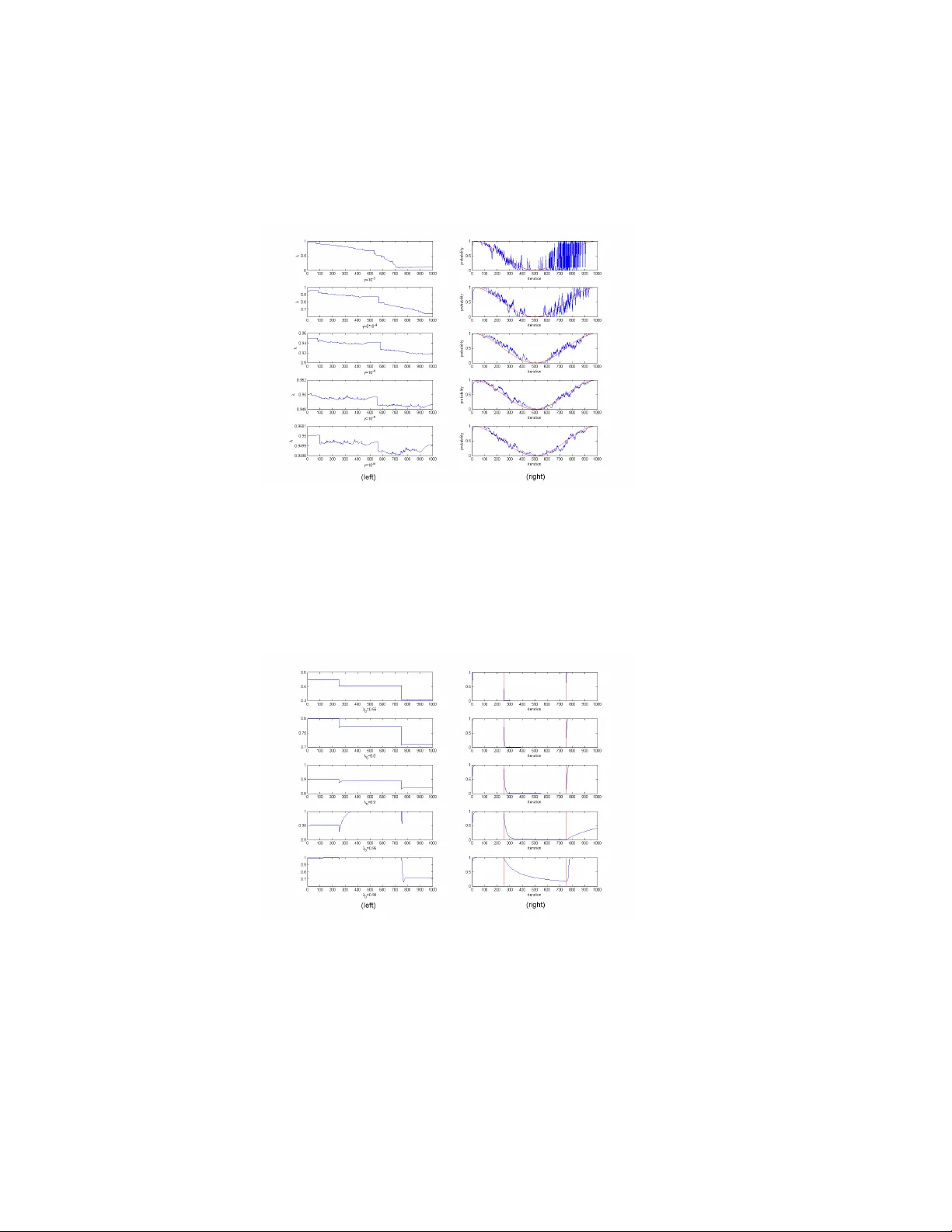
Adaptiv e F orgetting F actor Fictitious Pla y Mic halis Sm yrnakis ? 1 and Da vid S. Leslie 2 1 Sc ho ol of Ph ysics and Astronom y Univ ersity of Manchester,UK. michalis.smyrnakis@manchester.ac.uk 2 Departmen t of Mathematics Universit y of Bristol, UK. david.leslie@bris.ac.uk Abstract. It is no w well kno wn that decentralised optimisation can b e form ulated as a p oten tial game, and game-theoretical learning algorithms can b e used to find an optimum. One of the most common learning tec h- niques in game theory is fictitious play . Ho w ever fictitious play is founded on an implicit assumption that opp onen ts’ strategies are stationary . W e presen t a nov el v ariation of fictitious play that allows the use of a more realistic mo del of opp onen t strategy . It uses a heuristic approach, from the online streaming data literature, to adaptively up date the weigh ts assigned to recen tly observed actions. W e compare the results of the pro- p osed algorithm with those of sto c hastic and geometric fictitious play in a simple strategic form game, a vehicle target assignment game and a dis- aster managemen t problem. In all the tests the rate of con vergence of the prop osed algorithm was similar or b etter than the v ariations of fictitious pla y w e compared it with. The new algorithm therefore improv es the p erformance of game-theoretical learning in decentralised optimisation. 1 In tro duction Decen tralised optimisation is a crucial comp onen t of sensor netw orks [1, 2], dis- aster managemen t [3], traffic control [4] and sc heduling [5]. In eac h of these domains a com bination of computational and communication complexity render cen tralised optimisation approaches intractable. It is now w ell known that many decen tralised optimisation problems can b e form ulated as a potential game [6–8]. Hence the optimisation problem can b e recast in terms of finding a Nash equilib- rium of a potential game. An iterative decentralised optimisation algorithm can therefore b e considered a type of learning in games algorithm, and vice versa. Fictitious play is the canonical example of learning in games [9]. Under fic- titious pla y each play er maintains some b eliefs ab out his opp onen ts’ strategies, and based on these b eliefs he chooses the action that maximises his expected rew ard. The play ers then up date their b eliefs ab out opp onen ts’ strategies after observing their actions. Fictitious pla y conv erges to Nash equilibrium for certain kinds of games [9, 10] but in practice this conv ergence can b e very slow. This is ? Mic halis Smyrnakis is supported b y The Engineering and Ph ysical Sciences Researc h Council EPSRC (grant num b er EP/I005765/1). 2 b ecause it implicitly assumes that the other play ers use a fixed strategy in the whole game b y giving the same weigh t to every observed action. In [11] this problem was addressed b y using particle filters to predict opp o- nen ts’ strategies. The drawbac k of this approac h is the computational cost of the particle filters that render difficult the application of this metho d in real life applications. In this pap er we prop ose an alternative metho d which uses a heuristic rule to adapt the w eights of opponents’ strategies b y taking into account their re- cen t actions. W e observe empirically that this approach reduces the num b er of steps that fictitious play needs to conv erge to a solution, and hence the commu- nications o v erhead betw een the distributed optimisers that is required to find a solution to the distributed optimisation problem. In addition the computa- tional demand of the prop osed algorithm is similar to the classic fictitious play algorithm. The remainder of this paper is organised as follo ws. W e start with a brief description of game theory , fictitious play and sto c hastic fictitious pla y . Section 3 introduces adaptive forgetting factor fictitious play (AFFFP). The impact of the algorithm’s parameters on its p erformance is studied in Section 4. Section 5 presents the results of AFFFP for a climbing hill game, a v ehicle target as- signmen t game and a disaster managemen t simulation scenario. W e finish with a conclusion. 2 Bac kground In this section we in tro duce the relationship b et w een p oten tial games and decen- tralised optimisation, as well as the classical fictitious play learning algorithm. 2.1 P otential games and decentralised optimisation A class of games which maps naturally to the decentralised optimisation frame- w ork is strategic form games. The elements of a strategic form game are [12] – a set of play ers 1 , 2 , . . . , I , – a set of actions s i ∈ S i for each play er i ∈ I , – a set of joint actions, s = ( s 1 , s 2 , . . . , s I ) ∈ S 1 × S 2 × . . . × S I = S , – a pay off function u i : S → R for each play er i , where u i ( s ) is the utility that pla yer i will gain after a sp ecific joint action s has b een play ed. W e will often write s = ( s i , s − i ), where s i is the action of Play er i and s − i is the join t action of Pla yer i ’s opp onen ts. The rules that the pla yers use to select the action that they will pla y in a game are called strategies. A play er i chooses his actions according to a pure strategy when he selects his actions by using a deterministic rule. In the cases that he c ho oses an action based on a probabilit y distribution then he acts according to a mixed strategy . If we denote the set of all the probabilit y distributions ov er the 3 action space S i as ∆ i , then a mixed strategy of play er i is an elemen t σ i ∈ ∆ i . W e define ∆ as the set product of all ∆ i , ∆ = ∆ 1 × . . . × ∆ I . Then the joint mixed strategy σ = ( σ 1 , . . . , σ I ), is defined as an elemen t of ∆ and we will often write σ = ( σ i , σ − i ) analogously to s = ( s i , s − i ). W e will denote the exp ected utility a pla y er i will gain if he chooses a strategy σ i (resp. s i ), when his opponents c ho ose the join t strategy σ − i as u i ( σ i , σ − i ) (resp. u i ( s i , σ − i )). Man y decision rules can b e used by the pla y ers to choose their actions in a game. One of them is to choose their actions from a set of mixed strategies that maximises their exp ected utilit y given their b eliefs ab out their opp onen ts’ strategies. When Pla yer i ’s opp onen ts’ strategies are σ − i then the b est resp onse of play er i is defined as: B R i ( σ − i ) = argmax σ i ∈ ∆ i u i ( σ i , σ − i ) . (1) Nash [13], based on Kakutani’s fixed p oin t theorem, show ed that every game has at least one equilibrium. This equilibrium is a strategy ˆ σ that is a fixed p oin t of the b est resp onse correspondence, ˆ σ i ∈ B R i ( ˆ σ − i ) ∀ i . Thus when a joint mixed strategy ˆ σ is a Nash equilibrium then u i ( ˆ σ i , ˆ σ − i ) ≥ u i ( s i , ˆ σ − i ) for all i, for all s i ∈ S i . (2) Equation (2) implies that if a strategy ˆ σ is a Nash equilibrium then it is not p ossible for a pla yer to increase his utilit y by unilaterally c hanging his strategy . When all the play ers in a game select equilibrium actions using pure strategies then the equilibrium is referred as pure strategy Nash equilibrium. A particularly useful category of games for multi-agen t decision problems is the class of p oten tial games [10, 8, 7]. The utilit y function of an exact p oten tial game satisfies the following prop ert y: u i ( s i , s − i ) − u i ( ˜ s i , s − i ) = φ ( s i , s − i ) − φ ( ˜ s i , s − i ) (3) where φ is a p oten tial function and the ab o ve equality stands for every play er i , for every action s − i ∈ S − i , and for every pair of actions s i , ˜ s i ∈ S i . The p oten- tial function depicts the changes in the pla yers’ pay offs when they unilaterally c hange their actions. Ev ery p oten tial game has at least one pure strategy Nash equilibrium [10]. There may b e more than one, but at any equilibrium no pla yer can increase their reward, therefore the p oten tial function, through a unilateral deviation. W onderful life utility [6, 7] is a metho d to design the individual utilit y func- tions of a p oten tial game such that the global utilit y function of a decen tralised optimisation problem acts as the p oten tial function. Play er i ’s utilit y when a join t action s = ( s i , s − i ) is p erformed, is the difference in global utility obtained b y the play er selecting action s i in comparison with the global utilit y that would ha ve b een obtained if i had selected an (arbitrarily chosen) reference action s i 0 : u i ( s i , s − i ) = u g ( s i , s − i ) − u g ( s i 0 , s − i ) (4) 4 where u g is the global utility function. Hence the decentralised optimisation problem can be cast as a p oten tial game, and any algorithm that is prov ed to con verge to Nash equilibria will con verge to a join t action from which no pla yer can increase the global rew ard through unilateral deviation. 2.2 Fictitious Pla y Fictitious play is a widely used learning tec hnique in game theory . In fictitious pla y each pla yer chooses his action according to the best resp onse to his b eliefs ab out opp onen t’s strategy . Initially eac h pla yer has some prior beliefs about the strategies that his opp o- nen ts use to choose actions. The play ers, after each iteration, update their beliefs ab out their opponents’ strategy and pla y again the b est resp onse according to their b eliefs. More formally in the b eginning of a game play ers maintain some arbitrary non-negative initial weigh t functions κ j 0 , j = 1 , . . . , I that are updated using the form ula: κ j t ( s j ) = κ j t − 1 ( s j ) + I s j t = s j (5) for each j , where I s j t = s j =  1 if s j t = s j 0 otherwise. . The mixed strategy of opp onen t j is estimated from the following formula: σ j t ( s j ) = κ j t ( s j ) P s j κ j t ( s j ) . (6) Equations (5) and (6) are equiv alent to: σ j t ( s j ) =  1 − 1 t j  σ j t − 1 ( s j ) + 1 t j I s j t = s j (7) where t j = t + P s j ∈ S j κ j 0 ( s j ). Pla yer i c ho oses an action whic h maximises his exp ected pay offs giv en his b eliefs ab out his opp onen ts’ strategies. The main purp ose of a learning algorithm like fictitious pla y is to con verge to a set of strategies that are a Nash equilibrium. F or classic fictitious play (7) it has been pro ved [9] that if σ is a strict Nash equilibrium and it is play ed at time t then it will b e pla yed for all further iterations of the game. Also any steady state of fictitious pla y is a Nash equilibrium. F urthermore, it has b een pro ved that fictitious pla y conv erges for 2 × 2 games with generic pay offs [14], zero sum games [15], games that can b e solved using iterative dominance [16] and potential games [10]. There are also games where fictitious play do es not con verge to a Nash equilibrium. Instead it can b ecome trapp ed in a limit cycle whose perio d is increasing through time. An example of such a game is Shapley’s game [17]. A pla y er i that uses the classic fictitious pla y algorithm uses best responses to his b eliefs to choose his actions, so he c hooses his actions s i from his pure strategy space S i . Randomisation is allow ed only in the case that play ers are indifferent b et w een his av ailable actions, but it is very rare in generic pay off strategic form 5 games for a pla yer to b e indifferen t betw een the a v ailable actions [18]. Sto c hastic fictitious play is a v ariation of fictitious play where pla yers use mixed strategies in order to choose actions. This v ariation w as originally introduced to allo w con vergence of play ers’ strategies to a mixed strategy Nash equilibrium [9] but has the additional adv antage of introducing exploration into the pro cess. The most common form of smo oth b est resp onse of Pla y er i , B R i ( σ − i ), is the following [9]: B R ( σ − i )( s i ) = exp( u i ( s i , σ − i ) /ξ ) P ˜ s i exp( u i ( ˜ s i , σ − i ) /ξ ) (8) where ξ is the randomisation parameter. When the v alue of ξ is close to zero, a B R is close to B R and play ers exploit their action space, whereas large v alues of ξ result in complete randomisation [9]. Sto c hastic fictitious play is a mo dification of fictitious pla y under which Pla yer i uses B R i ( σ − i t ) to randomly select an action instead of selecting a best resp onse action B R i ( σ − i t ). W e reinforce the fact that the difference betw een clas- sic fictitious play and sto c hastic fictitious play is in the decision rule the pla yers use to c hoose the actions. The updating rule (7) that is used to update the b eliefs of the opp onen ts’ strategies are the same in both algorithms. When Play er i uses equation (7) to up date the b eliefs about opp onen ts’ strategies he treats the en vironmen t of the game as stationary and implicitly assumes that the actions of the play ers are sampled from a fixed probability distribution [9]. Therefore recent obse r v ations ha ve the same w eight as initial ones. This approac h leads to p oor adaptation when other play ers change their strategies. A v ariation of fictitious pla y that treats the opponents’ strategies as dynamic and places greater weigh ts on recent observ ations while we calculate each action’s probabilit y is geometric fictitious play , introduced in [9]. According to this v ari- ation of fictitious play the estimation of each opp onen t’s probability to pla y an action s j is ev aluated using the formula: σ j t ( s j ) = (1 − z ) σ j t − 1 ( s j ) + z I s j t = s j (9) where z ∈ (0 , 1) is a constan t. In Section 3 we in tro duce a new v ariant of fictitious play in whic h the constant z is automatically adapted in resp onse to the observ ations of opp onen t strategy . 3 Adaptiv e forgetting factor fictitious pla y The ob jective of pla y ers when they maintain beliefs σ − i t is to estimate the mixed strategy of opp onen ts. How ev er consider streaming data where in each time step a new observ ation arrives and it b elongs to one of J a v ailable classes [19]. When the ob jective is to estimate the probabilit y of each class giv en the observ ed data, this ob jective can b e expressed as the fitting of a m ultinomial distribution to the 6 observ ed data stream. If a fixed m ultinomial distribution o ver time is assumed, then its parameters can b e estimated using the empirical frequencies of the previously observ ed data. This is exactly the strategy estimation describ ed in Section 2.2. But in real life applications it is rare to observ e a data stream from a constan t distribution. Hence there is a need for the learning algorithm to adapt to the distribution that the data curren tly follow. This is similar to iterative games, where w e exp ect that all play ers update their strategies simultaneously . An approach that is widely used in the streaming data literature to handle c hanges in data distributions is forgetting. This suggests that recen t observ ations ha ve greater impact on the estimation of the algorithm’s parameters than the older ones. Two metho ds of forgetting are commonly used: windo w based meth- o ds and resetting. Salgado et.al [20] sho wed that when abrupt changes (jumps) are detected then the optimal p olicy is to reset the parameters of the algorithm. In the case of smooth changes (drift) in the data stream’s distribution, a solution is to use only a segmen t of the data (a window). The simplest form of windo w based metho ds uses a sp ecific segment size constantly; there are also approac hes that adaptiv ely c hange the size of the window but they are more complicated. Some examples of algorithms that use windo w based metho ds are [21–23]. Another metho d is to introduce forgetting, which is also used in geometric fictitious play (9), to discount the old information by giving higher weigh ts to the recent observ ations. When the discoun t parameter is fixed it is necessary to kno w a priori the distribution of data and the w ay that they ev olve th rough time due to the fact that we m ust choose the forgetting factor in adv ance. In addition the p erformance of the appro ximation when there are changes that result from a jump or non-constan t drift is p oor for a fixed forgetting factor. F or those reasons this metho dology has serious limitations. A more sophisticated solution is the use of a forgetting factor that tak es in to accoun t the recent data and the previously estimated parameters of the mo del and adapts to observed c hanges in the data distribution. Suc h a forgetting factor was proposed by Ha ykin [24] in the case of recursive least squares filtering problems. In [24] the ob jectiv e was the minimisation of the mean square error of a cost function that dep ends on an exp onen tial weigh ting factor λ . This forgetting factor is then recursiv ely up dated using gradien t descent of the forgetting factor, λ , with respect to the residual errors of the algorithm. Anagnostopoulos [19] prop osed a generalisation of this metho d in the context of online streaming data from a generalised linear mo del according to which the forgetting factors are adaptiv ely changed by using gradien t ascen t of the log-likelihoo d of the new data p oin t. In the streaming data context, after t time interv als we observ e a sequence of data x 1 , . . . , x t and we fit a mo del f ( θ t | x 1: t ), where θ t are the model’s parameters at time t . Note that the parameters of the mo del, θ t , dep end on the observ ed data stream x 1: t and the forgetting factors λ t . Since the estimated mo del parameters dep end on λ t w e will write θ t ( λ t ). The log-likelihoo d of the data that will arrive at time t + 1, x t +1 , giv en the parameters of the mo del at time t will b e denoted as 7 L ( x t +1 ; θ t ( λ t )). Then the up date of the forgetting factor λ t +1 can b e expressed as: λ t +1 = λ t + γ ∂ L ( x t +1 ; θ t ( λ t )) ∂ λ (10) where γ is the learning rate parameter of the gradient ascent algorithm. As in [19], w e can apply the forgetting factor of equation (10) in the case of fitting a m ultinomial distribution to streaming data. This will result a new up date rule that pla y ers can use, instead of the classic fictitious play update rule (7), to main tain b eliefs ab out opp onen ts’ strategies. In classic fictitious pla y the w eight function (5) places the same weigh t on ev ery observed action. In particular κ j t ( s j ) denotes the num b er of times that pla yer j has pla yed the action s j in the game. T o introduce forgetting the impact of the previously observed actions in the w eight function will b e discoun ted by a factor λ t − 1 . Such a weigh t function can b e written as: κ j t ( s j ) = λ j t − 1 κ j t − 1 ( s j ) + I s j t − 1 = s j (11) where I s j t − 1 = s j is the same identit y function as in (7). T o normalise w e set n t = P s j ∈ S j κ j t ( s j ). F rom the definition of κ j t ( s j ) w e can use the following recursion to ev aluate n j t n j t = λ j t − 1 n j t − 1 + 1 . (12) Then play er i ’s beliefs about his opponent j ’s probability of playing action s j will b e: σ j t ( s j ) = κ j t ( s j ) n j t . (13) Similarly to the case of geometric fictitious pla y 0 < λ t ≤ 1. Moreov er when the v alue of λ t is close to zero this results in very fast adaptation and when λ t = 0 the pla yers are my opic, and th us they resp ond to the last action of their opp onen ts. On the other hand when λ t = 1 this results in the classic fictitious pla y up date rule. F rom this p oin t on in we will only consider inference ov er a single opp onen t mixed strategy in fictitious play . In the case of multiple opponents separate estimates are formed identically and indep enden tly for eac h opponent. W e will therefore drop all dependence on pla yer i , and write s t , σ t and κ t ( s ) for the opp onen t’s action, strategy and w eight function resp ectiv ely . The v alue of λ should be updated in order to hav e adaptive forgetting factors. Initially we hav e to ev aluate the log-likelihoo d of the recently observed action s t giv en the b eliefs of the opp onen ts strategies. The log-likelihoo d is of the follo wing form: L ( s t ; σ t − 1 ) = ln σ t − 1 ( s t ) (14) When we replace σ t − 1 ( s t ) with its equiv alen t from (13) the log-lik eliho od can b e written as: L ( s t ; σ t − 1 ) = ln  κ t − 1 ( s t ) n t − 1  = ln κ t − 1 ( s t ) − ln n t − 1 (15) 8 In order to estimate the update of λ , equation (10), the ev aluation of the log-lik eliho od’s deriv ative with respect to λ is required. The terms κ t and n t b oth dep end on λ . Hence the deriv ative of (15) is: ∂ L ( s t ; σ t − 1 ) ∂ λ = 1 κ t − 1 ( s t ) ∂ ∂ λ κ t − 1 ( s t ) − 1 n t − 1 ∂ ∂ λ n t − 1 (16) Note that κ t ( s t ) = λ t − 1 κ t − 1 ( s t ) + I s j t − 1 = s j , so ∂ ∂ λ κ t ( s ) | λ = λ t − 1 = κ t − 1 ( s ) + λ t − 1 ∂ ∂ λ κ t − 1 ( s ) | λ = λ t − 1 (17) and similarly ∂ ∂ λ n t | λ = λ t − 1 = n t − 1 + λ t − 1 ∂ ∂ λ n t − 1 | λ = λ t − 1 (18) W e can use equations (17) and (18) to recursively estimate ∂ ∂ λ κ t − 1 ( s ) for eac h s and ∂ ∂ λ n t − 1 and hence calculate ∂ ∂ λ L ( s t ; σ t − 1 ). Summarising we can ev aluate the adaptive forgetting factor λ t as follows: λ t = λ t − 1 + γ  1 κ t − 1 ( s ) ∂ ∂ λ κ t − 1 ( s ) − 1 n t − 1 ∂ ∂ λ n t − 1  (19) T o ensure that λ t remains in (0, 1) we truncate it to this interv al whenever it leav es. After up dating their b eliefs play ers can choose their actions by c ho osing either a b est response to their b eliefs of their opp onen ts strategies or a smo oth b est resp onse. T able 1 summarises the algorithm of adaptiv e forgetting factor fictitious play . A t time t , each play er carries out the follo wing 1. Up dates the weigh ts κ j t ( s j ) = λ j t − 1 κ j t − 1 ( s j ) + I s j t − 1 = s j 2. Up date ∂ ∂ λ κ j t − 1 ( s ) and ∂ ∂ λ n j t − 1 using equations (17) and (18) 3. Based on the weigh ts of step 1 eac h pla y er updates his b eliefs about his opponents strategies using σ j t ( s j ) = κ j t ( s j ) n j t , where n j t = λ j t − 1 n j t − 1 + 1. 4. Cho ose an action based on the b eliefs of step 3 according either to b est response, B R , or to smo oth best resp onse B R 5. Observ e opp onen t’s action s j t 6. Up date the forgetting factor using: λ j t = λ j t − 1 + γ  1 κ j t − 1 ( s ) ∂ ∂ λ κ j t − 1 ( s ) − 1 n j t − 1 ∂ ∂ λ n j t − 1  T able 1. Adaptive forgetting factor fictitious play algorithm 9 4 AFFFP parameters The adaptive rule that we choose to update the forgetting factor λ is based on the gradien t ascent algorithm. It is w ell known that different initial v alues of an algorithm’s parameter and learning rates γ can lead to po or results of the gradien t ascen t algorithm [25]. This is because v ery small v alues of γ lead to p oor exploration of the space and thus the gradient ascent algorithm can be trapp ed in an area where the solution is not optimal, whereas large v alues of γ can result in big jumps that will lead the algorithm aw ay from the area of the optimum solution. Thus we should ev aluate the p erformance of adaptive forgetting factor fictitious pla y for different combinations of the step size parameter γ and initial v alues λ 0 . W e employ ed a to y example, where a single opp onen t chooses his actions us- ing a mixed strategy whic h has a sin usoidal form, a situation which corresp onds to smo oth changes in the data distribution of online streaming data. The opp o- nen t uses a strategy of the following form ov er the t = 1 , 2 , . . . 1000 iterations of the game: σ t (1) = cos 2 πt β +1 2 = 1 − σ t (2), where β = 1000. W e rep eated this example 100 times for eac h combination of γ and λ 0 . Each time we measured the mean square error of the estimated strategy against the real one. The range of γ and λ 0 w as 10 − 6 ≤ γ ≤ 10 − 1 and 10 − 1 ≤ λ 0 ≤ 1 resp ectiv ely . (a) Contour plot of mean square er- ror when the range of γ and λ is 10 − 6 ≤ γ ≤ 10 − 1 and 10 − 1 ≤ λ ≤ 1 resp ectiv ely . (b) Contour plot of mean square error when the range of γ and λ is 10 − 6 ≤ γ ≤ 5 × 10 − 3 and 0 . 6 ≤ λ ≤ 1 resp ectiv ely Fig. 1. Contour plot of mean square error The av erage mean square error for all the combinations of γ and λ 0 is depicted on Figure 1. The mean square error is minimised in the dark area of the contour plot. In Figure 1(a) we observe that when γ is less than 10 − 3 and λ 0 is greater than 0 . 6 the mean square e rr or is minimised. In Figure 1(b) we reduce the range of γ and λ 0 to b e 10 − 6 ≤ γ ≤ 5 × 10 − 3 and 0 . 6 ≤ λ 0 ≤ 1, resp ectiv ely . V alues of λ 0 greater than 0.75 result in estimators with small mean square error, for certain v alues of γ , and as the v alue of λ 0 approac hes 0.95 so it is minimised for a wider range of learning rates. W e also observe that when λ 0 is greater than 0.98 and 10 as w e approach 1 then the mean square error increases. This suggests that for v alues of λ 0 greater than 0 . 98 the v alue of λ app oac hes 1 very fast and th us the algorithm behav es like the classic fictitious play up date rule. In contrast when λ 0 is less than 0.75 then w e introduce big discoun ts to the previously observed actions from the b eginning of the game and the play ers easily use strategies that are reactions to their opp onen t’s randomisation. In addition, indep enden tly from the initial v alue of λ 0 , when the learning rate γ , is greater than 0.001 the algorithm results in p oor estimations of the opp onen t’s strategy . This is b ecause for γ greater than 0.001 the step that a play er mov es tow ards the maximum of the log-lik elihoo d is v ery large and that results in v alues of λ whic h are close either to zero or to one. So the pla yer uses either the classic fictitious play up date rule or resp onds to his opp onen t’s last observed action. W e further examine the relationship betw een the performance of adaptiv e forgetting factor fictitious play and the sequence of λ ’s in the drift to y example with resp ect to the initial v alues of the parameters λ 0 and γ . W e use tw o in- stances of the drift to y example. In the first one we set a fixed v alue of parameter γ = 10 − 4 and examine the p erformance of our algorithm and the evolution of λ during the game for different v alues of λ 0 = { 0 . 55 , 0 . 8 , 0 . 9 , 0 . 95 , 0 . 99 } . In the second one we fix λ 0 and examined the results of the algorithm for different v al- ues of γ = { 10 − 6 , 10 − 5 , 5 · 10 − 4 , 10 − 4 , 10 − 3 } . Figures 2 and 3 depict the results of the case of fixed γ and λ 0 , resp ectiv ely . Eac h row of these figures consists of tw o plots for the same set of parameters, γ and λ 0 . The left figure shows the ev olution of λ during the game and the righ t one depicts the pre-sp ecified strategy of the opp onen t and its corresponding prediction. As we observe in Figure 2, when we set λ 0 = 0 . 55 the tracking of the op- p onen t’s strategy was affected by his randomisation. The v alue of λ constantly decreases which results in giving higher weigh ts to the recently observed actions ev en if they are a consequence of randomisation. When w e increase the v alue of λ 0 to 0.8 the results are improving. When we increase λ 0 to 0.90 or 0.95 the resulting sequence of λ ’s do es not affect the tracking of opp onen t’s strategy . On the other hand when w e increase the v alue of λ 0 to 0.99 the v alue of λ is v ery close to 1 for man y iterations which result in p oor approximation for the same reasons that the classic fictitious play up date rule fails to capture smo oth c hanges in opp onen t’s strategy . When λ 0 is decreased to 0.9 the appro ximation of opp onen t’s strategy improv es significantly . Figure 3 depicts the results when λ 0 = 0 . 95 for different v alues of parameter γ . W e observe that high v alues of γ ( γ = 10 − 3 , 5 · 10 − 4 ) result in big c hanges in the v alue of λ and that affects the qualit y of the approximation. On the other hand when w e use v ery small v alues of γ , γ = 10 − 5 , or γ = 10 − 6 , it leads to v ery small deviations from λ 0 . The goo d appro ximation results of opp onen t’s strategy that we observ e for those tw o v alues of γ are b ecause of the initial v alue λ 0 . In this scenario if we fix the v alue of λ = 0 . 95 during the whole game we will also hav e a go od appro ximation. But in real life applications it is imp ossible to c ho ose so efficiently the v alue of λ 0 . When γ = 10 − 4 w e observe changes in the 11 v alues of λ , which are not so sudden as the ones for γ = 10 − 3 or γ = 5 · 10 − 4 , that lead to go od approximation of opp onen t’s strategy . Fig. 2. Evolution of λ and tracking of σ t (1) when the true strategies are mixed when γ is fixed. The pre-sp ecified strategy of the opponent and its prediction are depicted as the red and blue line resp ectiv ely . W e also performed simulations for a case where jumps occur. In this ex- ample we used a game of 1000 iterations and tw o a v ailable actions, 1 and 2. The opp onen t play ed action 1 with probability σ 2 t (1) = 1 during the first 250 and the last 250 iterations of the game and for the remaining iterations of the game σ 2 t (1) = 0. The probability of the second action can b e calculated by using σ 2 t (2) = 1 − σ 2 t (1). The results for the case of fixed γ and λ 0 are depicted in Figures 4 and 5, resp ectiv ely . When abrupt changes o ccur the differen t v alues of γ do not affect the per- formance of the algorithm as w e observe in Figure 5. On the contrary the initial v alue of λ affects the estimation of the jumps in the opp onen t’s strategies. As w e observe in Figure 4 the opp onen t’s strategy approximation and the evolution of λ are similar when λ 0 is equal to 0.55, 0.8 and 0.9 resp ectiv ely . In those three cases when a jump is observed, there is a drop in the v alue of λ , then λ sligh tly increases and finally it remains constant until the next jump o ccurs. The sequences of λ and the appro ximation results of the last tw o cases, λ 0 = 0 . 95 and λ 0 = 0 . 99 are differen t from the 3 cases we describ ed ab o ve. In b oth of them the opp onen t’s strategy tracking is go od at the first 250 iterations, but afterwards these tw o examples hav e the opp osite b eha viour. In the example where λ 0 = 0 . 95 the opp onen t’s strategy is correctly appro ximated when σ t (1) = 0. Because of the high weigh ts of the previously observ ed actions, the likelihoo d needs a large n umber of iterations to b ecome constan t and thus λ b ecomes equal to 1. Then the adaptiv e forgetting factor fictitious pla y process becomes iden tical 12 Fig. 3. Evolution of λ and tracking of σ t (1) when the true strategies are mixed when λ 0 is fixed. The pre-sp ecified strategy of the opp onen t and its prediction are depicted as the red and blue line resp ectiv ely Fig. 4. Evolution of λ and tracking of σ t (1) when the true strategies are pure when γ is fixed. The pre-specified strategy of the opponent and its prediction are depicted as the red and blue line resp ectiv ely . 13 Fig. 5. Evolution of λ and tracking of σ t (1) when the true strategies are pure when λ 0 is fixed. The pre-specified strategy of the opponent and its prediction are depicted as the red and blue line resp ectiv ely . to classic fictitious pla y and fails to adapt to the second jump. When λ 0 is equal to 0.99 adaptive forgetting factor fictitious pla y fails to adapt the estimation of opponent’s strategy to the first jump. But when the second jump o ccurs, the lik elihoo d of action 1 is small since action 2 is play ed for 500 consecutiv e iterations, and a drop in the v alue of λ is observed which resulted in adaptation to the c hange of opp onen t’s strategy . By taking in to account the ab o ve results we observe that γ = 10 − 4 and 0 . 8 ≤ λ 0 ≤ 0 . 9 leads to useful appro ximations when w e consider cases where b oth smo oth and abrupt changes in opp onen t’s strategy are p ossible to happ en. In the remainder of the article w e set γ = 10 − 4 and λ 0 = 0 . 8. 5 Results 5.1 Clim bing hill game W e initially compared the performance of the prop osed algorithm with the re- sults of geometric and classic sto c hastic fictitious play in a three pla yer climbing hill game. This game whic h is depicted in T able 2, generalises the climbing hill game that w as presen ted in [26] and exhibits a long b est resp onse path from the risk-dominan t join t mixed action (D,D,U) to the Nash equilibrium. W e present the results of 1000 replications of a learning episo de of 1000 iterations for each game. F or eac h replication of 1000 iterations we computed the mean pa yoff. After the end of the 1000 replications the ov erall mean of the 1000 pay off means was computed. The v alue of the learning parameter z of geometric fictitious pla y was set to 0 . 1. W e selected this v alue of z on the p emise that the algorithm has the 14 U M D U M D 0 0 0 0 50 40 0 0 30 U U M D -300 70 80 -300 60 0 0 0 0 M U M D 100 -300 90 0 0 0 0 0 0 D T able 2. Climbing hill game with three play ers. Pla yer 1 selects rows, Play er 2 selects columns, and Play er 3 selects the matrix. The global reward depicted in the matrices, is recived by all pla yers. The unique Nash equilibrium is in b old. b est results in the tracking experiment with pre-sp ecified opp onen ts strategy that w e used in Section 4 to select the parameters of AFFFP . Thus we will use this learning rate ia all the sim ulations that we present in the rest of this article. F or all algorithms we used smo oth b est resp onses (8) with randomisation parameter ξ in the smo oth b est resp onse function equal to 1, allowing the same randomisation for all algorithms. Adaptiv e forgetting factor fictitious pla y p erformed better than both geo- metric and sto c hastic fictitious play . The o verall mean global pay off was 95.26 for AFFFP whereas the resp ectiv e pay offs for geometric and sto c hastic fictitious pla y were 91.7 and 70.3. Sto c hastic fictitious play didn’t conv erge to the Nash equilibrium after 1000 replications. Also when we are concerned about the sp eed of conv ergence the proposed v ariations of fictitious play outperform geometric fictitious play . This can b e seen if we reduce the iterations of the game to 200. Then the ov erall mean pa yoffs of AFFFP is 90.12 when for geometric fictitious pla y it is 63.12. This is b ecause adaptive forgetting factor fictitious play requires appro ximately 100 iterations to reach the Nash equilibrium, when geometric fictitious play needs at least 300. This difference is depicted in Figure 6. Fig. 6. Probability of playing the (U,U,D) equilibrium for one run of eac h of AFFFP (blue dot line), geometric fictitious pla y (black solid line) and sto c hastic fictitious play (green diamond line) for the three play er climbing hill game. 15 5.2 V ehicle target assignment gam e W e also compared the p erformance of the prop osed v ariation of fictitious play against the results of geometric fictitious play in the vehicle target assignment game that is describ ed in [7]. In this game agents should co ordinate to ac hieve a common goal which is to maximise the total v alue of the targets that are destro yed. In particular in a sp ecific area we place I vehicles and J targets. F or eac h vehicle i , its a v ailable actions are simply the targets that are av ailable to engage. Each v ehicle can choose only one target to engage but a target can b e engaged b y man y v ehicles. The probabilit y that pla yer i has to destro y a target j is p ij if it chooses to engage target j . W e assume that the probability each agen t has to destroy a target is indep enden t of the actions of the other agents, and the target is destroy ed if an y one agent succesfully destro yes it, so the probabilit y a target j is destroy ed by the vehicles that engage it is 1 − Q i : s i = j (1 − p ij ). Eac h of the targets has a different v alue V j . The exp ected utilit y that is pro duced from the target j is the pro duct of its v alue V j and the probabilit y it has to b e destroy ed b y the vehicles that engage it. More formally we can express the utilit y that is pro duced from target j as: U j ( s ) = V j (1 − Y i : s i = j (1 − p ij )) (20) The global utilit y is then the sum of the utilities of eac h target: u g ( s ) = X j U j ( s ) . (21) W onderfull life utility w as used to to ev aluate each v ehicle’s pay off. Then the utilit y that a v ehicle i receives after engange a target j , s i = j , is u i ( s i , s − i ) = U j ( s i , s − i ) − U j ( s i 0 , s − i ) = (22) where s i 0 w as set to b e the greedy action of play er i : s i 0 = argmax j V j p ij . In our sim ulations we used thirt y vehicles and thirt y targets that were placed uniformly at random in a unit square. The probabilit y of a vehicle i to destroy a target j is prop ortional to the in verse of its distance from this target 1 /d ij . The v alues of the targets are independently sampled from a uniform distribution with range in [0 100]. The vehicles had to “negotiate” with the other vehicles (play ers) for a fixed n umber of negotiation steps before they c ho ose a target to engage. A negotiation step b egins with eac h play er c ho osing a target to engage and it ends by the agen ts exchanging this information with the others, and up dating their b eliefs ab out their opponents’ strategies based on this information. The target that eac h vehicle will c ho ose in the game will b e his action at the final negotiation step. Figure 7 depicts the a verage results for 100 instances of the game for the t wo algorithms, AFFFP and geometric fictitious play . F or eac h instance, b oth 16 algorithms run for 100 negotiation steps. T o b e able to av erage across the 100 instances w e normalise the scores of an instance by the highest observ ed score for that instance (since some instances will ha ve greater av ailable score than others). As in the strategic form game, we set the randomisation parameter ξ in the smo oth b est resp onse function equal to 1 for b oth algorithms. In Figure 7 w e observ e that AFFFP result in a better solution on av erage than geometric fictitious play . F urthermore geometric fictitious play needs more iterations to reac h the area where its rew ard is maximised than AFFFP . Fig. 7. Utilit y of AFFFP (dotted line) and geometric fictitious play (dashed line) for the vehicle target assignment game. 5.3 Disaster managemen t scenario Finally we test our algorithm in a disaster management scenario as describ ed in [27]. Consider the case where a natural disaster has happ ened (an earthquak e for example) and b ecause of this N I sim ultaneous incidents o ccurred in differen t areas of a town. In each incident j , a differen t num b er of p eople N p ( j ) are injured. The town has a sp ecific num b er of am bulances N amb a v ailable that are able to collect the injured p eople. An am bulance i can be at the area of inciden t j in time T ij and has capacit y c i . W e will assume that the total capacity of the ambulances is larger than the num b er of injured p eople. Our aim is to allo cate the am bulances to the incidents in such a w ay that the av erage time 1 N amb P i : s i = j T ij that the am bulances need to reac h the incidents is minimised while all the people that are engaged in the inciden t will b e sa ved. Then we can formulate this scenario as follows. Each of the N amb pla yers should c ho ose one of the N I inciden ts as actions. The utilit y to the system of an allo cation is: u g ( s ) = − 1 N amb N I X j =1 X i : s i = j T ij − N I X j =1 max  0 , N p ( j ) − X i : s i = j c i  (23) 17 where i = 1 , . . . , N amb and s i is the action of play er i . The emergency units ha ve to “negotiate” with eac h other and choose the incident which they will b e allo cated to, using a v arian t of fictitious pla y . The first component of the utilit y function expresses the first aim, to allo cate the ambulance to an incident as fast as p ossible. Thus the agents hav e to choose an incident with small T ij . The second ob jective, which is to sa ve all the injured p eople that are engaged in an inciden t, is expressed as the second comp onen t of the utility function. It is a penalty factor that adds to the av erage time the n umber of the p eople that were not able to be sa ved. Lik e the v ehicle target assignmen t game eac h play er can choose only one incident to help, but in each inciden t more than one play er can provide his help. W e follow [27] and consider simulations with 3 and 5 inciden ts, and 10, 15 and 20 a v ailable am bulances. W e run 200 trials for each of the combinations of am bulances and inciden ts, for eac h algorithm. Since this scenario is NP-complete [27] our aim is not to find the optimal solution, but to reac h a sufficien t or a near optimal solution. F urthermore the algorithm w e present here is “an y-time”, since the system utility generally increases as the time goes on, and therefore in terruption b efore termination results in goo d, if not optimal actions. In each of the 200 trials the time T ij that an ambulance needs to reach an inciden t is a random n umber uniformly distributed betw een zero and one. The capacity of each ambulance is an in teger uniformly distributed b et ween one and four. Finally the total n umber of injured p eople that are in volv ed in each inciden t is a uniformly distributed in teger betw een c t 2 ∗ N I and c t N I , where c t is the total capacit y of the emergency units c t = P N amb i =1 c i . In each trial we allo w 200 negotiation steps. In this scenario because of the utilit y function structure, a big randomisation parameter ξ in the smo oth b est resp onse function can easily lead to unnecessary randomisation. F or that reason w e set ξ to 0 . 01 for b oth algorithms which results in a decision rule which ap- pro ximates b est resp onse. The learning rate and the initial v alue of λ in adaptiv e forgetting factor is set to 10 − 4 and 0 . 8 resp ectiv ely . W e use the same performance measures as [27] to test the p erformance of our algorithms. W e compared the solution of our algorithm against the centralised solution which can b e obtained using binary in teger programming. In particular w e compared the solution of our algorithm against the one we obtain by using Matlab’s bintpr o g algorithm,which uses a branch and b ound algorithm that is based on linear programming relaxation [28–30]. T o compare the result of these t wo algorithms we u se the ratio f f p f opt , where f f p is the utilit y that the agents could gain if they used the v ariations of fictitious play w e prop ose and f opt is the utilit y that the agen ts should gain if they w ere using the solution of bintpr o g . Th us v alues of the ratio smaller than one mean that the prop osed v ariations of fictitious play p erform better than bintpr o g , and v alues of the ratio larger than one mean that the prop osed v ariations of fictitious play perform w orst than bintpr o g . F urthermore we measured the p ercen tage of the instances in which all the casualties are rescued, and the ov erall p ercen tage of p eople that are rescued. 18 %complete % sav ed f f p /f opt 10 ambulances 82.0 92.84 1.2702 3 incidents 15 ambulances 77.5 89.88 1.2624 20 ambulances 81.0 90.59 1.2058 10 ambulances 91.0 98.54 1.6631 5 incidents 15 ambulances 90.5 98.28 1.5088 20 ambulances 83.0 93.6 1.4251 T able 3. Results of adaptiv e forgetting factor fictitious play after 200 negotiation steps for the three p erformance measures. %complete % sav ed f f p /f opt 10 ambulances 95,5 99,74 1.2970 3 incidents 15 ambulances 74,5 88.24 1.2965 20 ambulances 60.55 87.9 1.2779 10 ambulances 94.5 99.68 1.8587 5 incidents 15 ambulances 79.0 88.28 1.7443 20 ambulances 48.50 86.54 1.8545 T able 4. Results of geometric fictitious pla y after 200 negotiation steps for the three p erformance measures. T ables 3 and 4 present the results w e hav e obtained in the last step of ne- gotiations b et ween the am bulances for the disaster management scenario when they use adaptive forgetting factor and geometric fictitious play resp ectiv ely , to co ordinate. The total p ercen tage of the p eople that were sav ed and the ratio of f f p /f opt w ere similar within the groups of 3 and 5 incidents when the adaptive forgetting factor fictitious play algorithm were used. Regarding the p ercen tage of the trials in whic h all people w ere sa ved, we can observ e that as w e increase the complexit y of the scenario, hence the num ber of ambulances, the p erformance of adaptive forgetting factor fictitious play is decreasing. When we compare the results of the tw o algorithms we can observe that in b oth cases of 3 and 5 inciden ts resp ectiv ely adaptiv e forgetting factor fictitious pla y p erform b etter than geometric fictitious pla y when the scenarios included more ambulances, and therefore were more complicated. Esp ecially in the case of the 20 ambulances the difference when w e consider the num b er of the cases where all the casualties were collected from the incidents, w as greater than 20%. The differences we can observe from bintpr o g ’s cen tralised solution, for b oth algorithms, can be explained from the structure of the utility function (23). The first comp onen t of the utility is a n umber b et w een zero and one since it is the a verage of the times, T ij , that the ambulances need to reach the incidents. On the other hand the p enalt y factor, ev en in the cases where only one p erson is not collected from the incidents, is greater than the first component of the utilit y . Th us a local searc h algorithm like the v ariations of fictitious pla y w e prop ose 19 initially searches for an allocation that collects all the injured p eople, so the p enalt y comp onen t of the utility will b e zero, and afterwards for the allo cation that minimises also the a verage time that the ambulances needed to reach the inciden ts. It is therefore easy to b ecome stuck in lo cal optima. W e hav e also examined how the results are influenced b y the num ber of iterations we use in eac h of the 200 trials of the game. F or that reason we hav e compared the results that w e would hav e obtained if in each instance of the sim ulations we had stopp ed the negotiations b et w een the emergency units after 50, 100, 150 and 200 iterations for b oth algorithms. T ables 5-7 and 8-10 depict the results for adaptive forgetting factor fictitious pla y and geometric fictitious pla y resp ectiv ely . Iterations 50 100 150 200 10 ambulances 74.5 81.0 82.0 82.0 3 incidents 15 ambulances 73.0 75.5 77.5 77.5 20 ambulances 73.5 78.0 80.0 81.0 10 ambulances 80.0 87.5 90.0 91.0 5 incidents 15 ambulances 76.5 84.5 89.5 90.5 20 ambulances 62.0 77.0 80.0 83.0 T able 5. Percen tage of solutions in which the capacit y of the am bulance in every inciden t w as enough to cov er all injured people for differen t stopping times of the negotiations, 50, 100, 150 and 200 iterations of the adaptiv e forgetting factor fictitious pla y algorithm. Iterations 50 100 150 200 10 ambulances 91.44 92.35 92.95 92.84 3 incidents 15 ambulances 88.65 90.28 89.97 89.88 20 ambulances 89.09 89.33 90.44 90.59 10 ambulances 96.39 97.80 98.51 98.54 5 incidents 15 ambulances 94.84 97.22 98.03 98.29 20 ambulances 87.61 91.90 92.81 93.61 T able 6. Average p ercen tage of injured p eople collected for different stopping times of the negotiations, 50, 100, 150 and 200 iterations of the adaptive forgetting factor fictitious play algorithm. W e can see from tables 5-7 that the performance of adaptiv e forgetting factor fictitious pla y , in all the measures that we used, is similar for 100, 150 and 200 negotiation steps. In particular when w e consider the percentage of the instances 20 Iterations 50 100 150 200 10 ambulances 1.2791 1.2603 1.2669 1.2702 3 incidents 15 ambulances 1.2701 1.2452 1.2319 1.2624 20 ambulances 1.2142 1.1971 1.1943 1.2058 10 ambulances 1.6989 1.6827 1.6772 1.6631 5 incidents 15 ambulances 1.5569 1.5352 1.5304 1.5088 20 ambulances 1.5298 1.4413 1.4306 1.4251 T able 7. Average p ercen tage of the ratio f f p /f opt for different stopping times of the negotiations, 50, 100, 150 and 200 iterations of the adaptiv e forgetting factor fictitious pla y algorithm. Iterations 50 100 150 200 10 ambulances 94.0 94.0 94.7 95.5 3 incidents 15 ambulances 71.0 73.0 73.3 74.5 20 ambulances 60.5 61.3 62.0 63.0 10 ambulances 86.0 92.0 93.3 94.5 5 incidents 15 ambulances 79.0 78.0 79.0 82.0 20 ambulances 42.0 49.0 47.3 48.5 T able 8. Percen tage of solutions in which the capacit y of the am bulance in every inciden t w as enough to cov er all injured people for differen t stopping times of the negotiations, 50, 100, 150 and 200 iterations of the geometric fictitious play algorithm. Iterations 50 100 150 200 10 ambulances 99.62 99.65 99.69 99.74 3 incidents 15 ambulances 88.20 88.21 88.21 88.24 20 ambulances 86.65 87.41 88.23 89.90 10 ambulances 97.20 99.54 99.61 99.68 5 incidents 15 ambulances 94.84 97.22 98.03 98.29 20 ambulances 85.33 86.38 86.391 86.54 T able 9. Average p ercen tage of injured p eople collected for different stopping times of the negotiations, 50, 100, 150 and 200 iterations of the geometric fictitious play algorithm. 21 Iterations 50 100 150 200 10 ambulances 1.2957 1.2928 1.3039 1.2970 3 incidents 15 ambulances 1.2965 1.3039 1.2801 1.2740 20 ambulances 1.2779 1.2744 1.2723 1.2722 10 ambulances 1.8587 1.8540 1.8550 1.8519 5 incidents 15 ambulances 1.7443 1.7205 1.7085 1.7074 20 ambulances 1.8545 1.7845 1.7744 1.7727 T able 10. Av erage p ercen tage of the ratio f f p /f opt for different stopping times of the negotiations, 50, 100, 150 and 200 iterations of the geometric fictitious play algorithm. that the ambulances collected all the injured p eople and the ratio f f p /f opt the difference in the results after 100 and 200 negotiation steps is b et ween 1% and 4.5%. The differences b ecome even smaller for the p ercen tage of the p eople that w ere sa ved which was less than 2%. Geometric fictitious pla y w as trapp ed in an area of a lo cal minimum after few iterations since the results are similar after 50, 100, 150 and 200 iterations. This is reflected in the results where geometric fictitious play p erformed worse than adaptiv e forgetting factor fictitious play especially in the complicated cases where the negotiations where b et w een 20 ambulances. Adaptiv e forgetting factor fictitious play p erformed also better than the Ran- dom Neural Netw ork (RNN) presented in [27], when we consider the p ercen tage of the cases in whic h all the injured p eople are collected and the ov erall p ercen t- age of p eople that are rescued. The p ercen tage of instances where the prop osed allo cations by the RNN could collect all the casualties were from 25 to 69 per- cen t. The corresp onding results of adaptiv e forgetting factor fictitious play are from 77 . 5 to 94 . 5. The ov erall p ercen tage of p eople that are rescued by the RNN algorithm are similar to the ones of adaptiv e forgetting factor fictitious play , b et w een 85 and 98 . 5 p ercen t. The ratio f f p f opt rep orted by [27] is b etter than that sho wn here. Ho wev er in [27] only the examples in which all the casualties were collected w ere included to ev aluate the ratio. Cases with high penalties, since the uncollected casualties introduce higher p enalties than the inefficient allo cation, w ere excluded from the ratio ev aluation. Thus artificially improv e their metric, esp ecially when one considers that in many instances less than 40% of their solutions were included. 6 Conclusions Fictitious pla y is a classic learning algorithm in games, but it is formed on an (incorrect) stationarity assumption. Therefore w e hav e introduced a v ariation of fictitious play , adaptiv e forgetting factor fictitious play , which address this prob- lem by giving higher weigh ts to the recently observed actions using a heuristic rule from the streaming data literature. 22 W e examined the impact of adaptive forgetting factor fictitious pla y parame- ters λ 0 and γ on the results of the algorithm. W e show ed that these tw o param- eter should be c hosen carefully since there are com binations of λ 0 and γ that induce v ery p oor results. An example of such com bination is when high v alues of the learning rate γ are combined with low v alues of λ 0 . This is b ecause v alues of λ 0 < 0 . 6 assign small w eights to the previously observed actions and this results in v olatile estimations that are influenced by opp onen ts’ randomisation. High v alues of the learning rate γ , mean that λ 0 is driven still low er, exacerbating the problem further. F rom the sim ulation results we hav e seen that a satisfactory com bination of parameters λ 0 and γ is 0 . 8 ≤ λ 0 ≥ 0 . 9 and γ = 10 − 4 . Adaptiv e forgetting factor p erformed b etter than the competitor algorithms in the clim bing hill game. Moreo ver it conv erged to the a b etter solution than geometric fictitious play in the v ehicle target assignment game. In the disaster managemen t scenario the performance of the proposed v ariation of fictitious pla y compared fav orably with that of geometric fictitious pla y and a pre-planning algorithm that uses neural net works [27]. Our empirical observ ations indicate that adaptive forgetting factor fictitious pla y conv erges to a solution that is at least as go od as that given b y the com- p etitor algorithms. Hence b y slightly increasing the computational intensit y of fictitious play less comm unication is required b et ween agen ts to quickly co ordi- nate on a desirable solution. References 1. Kho, J., Rogers, A., Jennings, N.R.: Decentralized control of adaptiv e sampling in wireless sensor netw orks. A CM T rans. Sen. Netw. 5 (3) (2009) 1–35 2. Lesser, V., Ortiz, C., T ambe, M., eds.: Distributed Sensor Netw orks: A Multiagen t P ersp ectiv e. Klu wer Academic Publishers, Boston (May 2003) 3. Kitano, H., T odokoro, S., No da, I., Matsubara, H., T ak ahashi, T., Shinjou, A., Shimada, S.: Robo cup rescue: Searc h and rescue in large-scale disasters as a domain for autonomous agen ts research. In: Proc. of IEEE Conf. on System, Man and Cyb ernetics. (1999) 4. v an Leeuw en, P ., Hesselink, H., Rohlinga, J.: Scheduling aircraft using constraint satisfaction. Electronic Notes in Theoretical Computer Science 76 (2002) 252 – 268 5. Stranjak, A., Dutta, P .S., Eb den, M., Rogers, A., Vytelingum, P .: A multi-agen t sim ulation system for prediction and scheduling of aero engine ov erhaul. In: AA- MAS ’08: Pro ceedings of the 7th In ternational joint Conference on Autonomous Agen ts and Multi-Agent Systems. (2008) 81–88 6. T umer, K., W olp ert, D.: A survey of collectives. In: Collectives and the Design of Complex Systems, Springer (2004) 1–42 7. Arslan, G., Marden, J., Shamma, J.: Autonomous vehicle-target assignment: A game theoretical formulation. Journal of Dynamic Systems, Measuremen t, and Con trol 129 (2007) 584–596 8. Chapman, A.C., Rogers, A.C., Jennings, N.R., Leslie, D.S.: A unifying frame- w ork for iterativ e approximate best resp onse algorithms for distributed constraint optimisation problems. The Knowledge Engineering Review (forthcoming). 23 9. F udenberg, D., Levine, D.: The Theory of Learning in Games. The MIT Press (1998) 10. Monderer, D., Shapley , L.: P otential games. Games and Economic Beha vior 14 (1996) 124–143 11. Sm yrnakis, M., Leslie, D.S.: Dynamic Opp onen t Mo delling in Fictitious Pla y. The Computer Journal (2010) 2308–2324 12. F udenberg, D., Tirole, J.: Game Theory . MIT Press (1991) 13. Nash, J.: Equilibrium p oin ts in n-p erson games. In: Pro ceedings of the National Academ y of Science, USA. V olume 36. (1950) 48–49 14. Miy asaw a, K.: On the conv ergence of learning pro cess in a 2x2 non-zero-p erson game (1961) 15. Robinson, J.: An iterative metho d of solving a game. Annals of Mathematics 54 (1951) 296–301 16. Nac hbar, J.H.: Evolutionary selection dynamics in games: Con vergence and limit prop erties. International Journal of Game Theory 19 (1) (1990) 59–89 17. Shapley , L.: Adv ances in Game Theory . Princeton Univ ersity Press, Princeton (1964) 18. F udenberg, D., Kreps, D.M.: Learning mixed equilibria. Games and Economic Beha vior 5 (1993) 320–367 19. Anagnostop oulos, C.: A Statistical F ramework for Streaming Data Analysis. PhD thesis, Imp erial College London (2010) 20. Salgado, M.E., Go o dwin, G.C., Middleton, R.H.: Mo dified least squares algorithm incorp orating exp onen tial resetting and forgetting. International Journal of Con- trol 47 (1988) 477–491 21. Blac k, M., Hick ey , R.J.: Maintaining the p erformance of a learned classifier under concept drift. In telligent Data Analysis 3 (6) (1999) 453 – 474 22. Muhlbaier, M., P olik ar, R.: An ensem ble approach for incremen tal learning in nonstationary environmen ts. In: Multiple Classifier Systems. (2007) 490–500 23. Aggarw al, C., Han, J., W ang, J., Y u, P .: On demand classification of data streams. In: Proceedings of the ten th A CM SIGKDD international conference on Knowledge Disco very and Data Mining. (August 2004) 503–508 24. Ha ykin, S.: Adaptiv e Filter Theory . Pren tice Hall (1996) 25. Bishop, C.M.: Neural Net works for Pattern Recognition. Oxford Universit y Press (1995) 26. Claus, C., Boutilier, C.: The dynamics of reinforcement learning in co operative m ultiagent systems. In: AAAI ’98/IAAI ’98: Pro ceedings of the fifteenth na- tional/ten th conference on Artificial in telligence/Innov ative applications of arti- ficial intelligence. (1998) 746–752 27. Gelen b e, E., Timotheou, S.: Random neural net works with synchronized interac- tions. Neural Computation 20 (2008) 2308–2324 28. W olsey , L.A.: In teger Programming. John Wiley & Sons (1998) 29. Nemhauser, G.L., W olsey , L.A.: In teger and Combinatorial Optimization. John Wiley & Sons (1988) 30. Hillier, F.S., Lieb erman, G.: Introduction to Op erations Research. McGra w-Hill (2001)