Algorithmic and topological aspects of semi-algebraic sets defined by quadratic polynomial

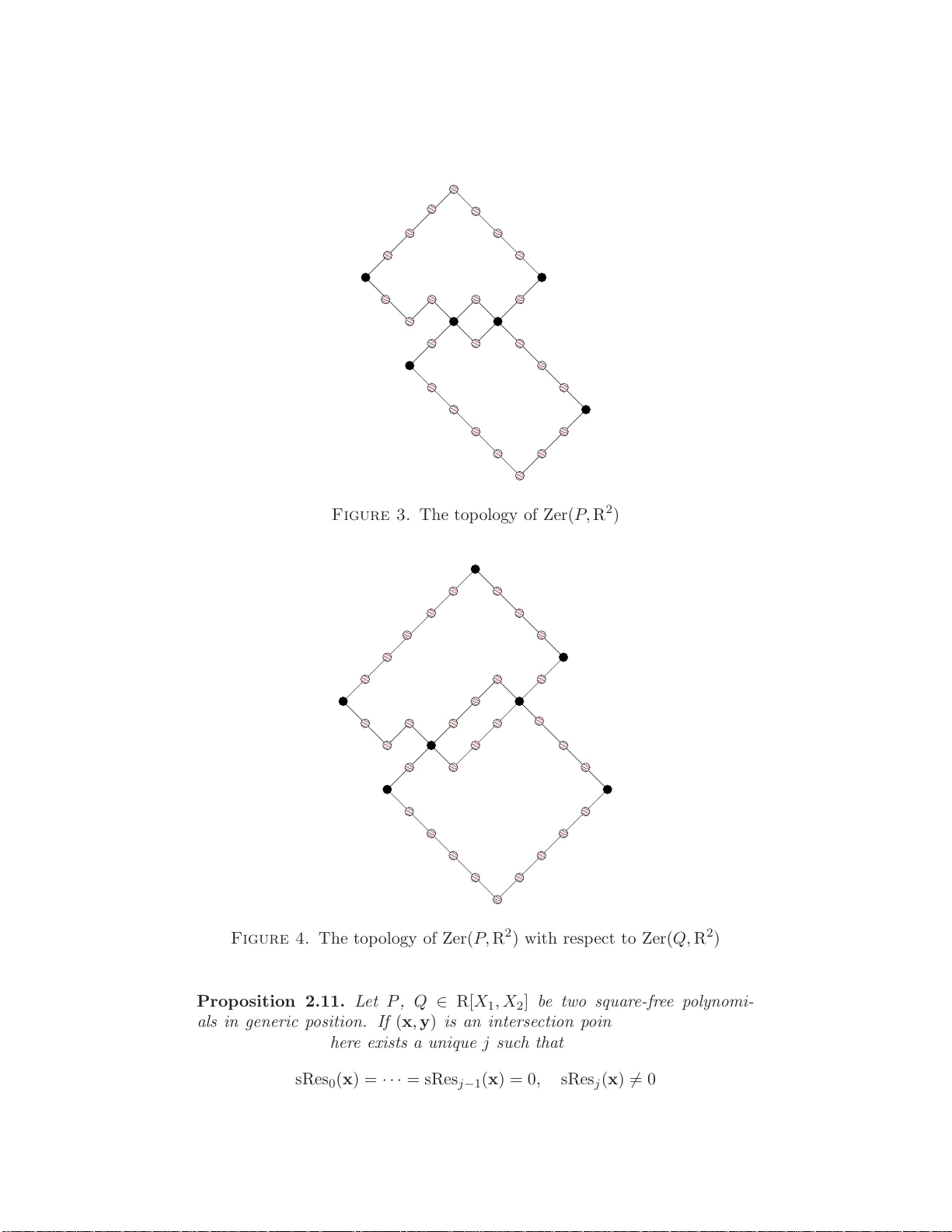
Algorith mic and top ological asp ects of semi-algebraic sets deﬁne d b y quadratic p o l ynomials Mic hael Kettner E-mail addr ess : mkettner @gatech.e du School of Ma thema tics, Georgia Institute of Technol ogy This do cument is the ﬁ nal version of th e my Ph.D. thesis for arc h iv al on arXiv.org. The orginal version w ill b e a v ailable in Decem b er 2007 at http://e td.gatech .edu/theses/available/etd- 08212007- 1 42510/ . iii F or my Mum and the memory of my D ad Con ten ts Summary vii Ac kn o wledgemen ts ix List of Figures xi List of T ables xiii Chapter 1. In tro duction 1 1. Rea l Algebraic Geometry 1 2. Be tti n umbers 2 3. Ho motop y T yp es 4 4. Arrangemen ts 5 5. Revie w of th e Results 6 Chapter 2. Mathematica l P r eliminaries 9 1. Rea l Algebraic Geometry 9 2. Alg ebraic T opology 21 3. The T op ology of Algebraic an d S emi-Algbraic Sets 28 Chapter 3. Bounding the Betti Num b ers 35 1. Results 35 2. Proof Strategy 36 3. Constructing Non-singular Complete Inte rsections 36 4. Proof of Theorem 3.1 37 Chapter 4. Bounding the Numb er of Homotop y Types 41 1. Result 41 2. Proof Strategy 42 3. T opology of Sets Deﬁned by Quadratic Con s train ts 42 4. P artitioning the Pa rameter Space 50 5. Proof of the Result 56 6. Me tric upp er b ound s 63 Chapter 5. Algorithms and Their Imp lemen tatio n 65 1. Computing the Betti Num b ers of Ar rangemen ts 65 2. Computing the Real I n tersection of Quadratic S urfaces 73 Bibliograph y 89 v vi CONTENTS Vita 95 Summary In th is th esis, w e consider semi-algebraic sets o v er a r eal closed ﬁeld R deﬁned by quadr atic p olynomials. Semi-algebraic sets of R k are d eﬁned as the smallest family of sets in R k that con tains the algebraic sets as w ell as the sets deﬁned by p olynomial inequ alities, and wh ic h is also closed un der the b o olean op erations (complemen tation, ﬁnite unions and ﬁn ite in tersections). W e pr o v e th e follo wing new b oun ds on th e top olog ical complexit y of semi- algebraic sets ov er a real closed ﬁeld R deﬁ n ed by qu adratic p olynomials, in terms of th e parameters of the system of p olynomials d eﬁning them, whic h impro v e th e known resu lts. (1) Let S ⊂ R k b e deﬁned b y P 1 ≥ 0 , . . . , P m ≥ 0 with P i ∈ R[ X 1 , . . . , X k ], m < k , and deg ( P i ) ≤ 2, for 1 ≤ i ≤ m . W e pro v e th at b i ( S ) ≤ 3 2 ·  6 ek m  m + k , 0 ≤ i ≤ k − 1. (2) Let P = { P 1 , . . . , P m } ⊂ R[ Y 1 , . . . , Y ℓ , X 1 , . . . , X k ], with deg Y ( P i ) ≤ 2, d eg X ( P i ) ≤ d , 1 ≤ i ≤ m . Let S ⊂ R ℓ + k b e a semi-algebaic set, deﬁned b y a Bo olean formula without negations, whose atoms are of the form, P ≥ 0 , P ≤ 0 , P ∈ P . Let π : R ℓ + k → R k b e the pro jection on the last k co-ordinates. W e pr ov e that the num b er of stable h omotop y t yp es amongst the ﬁb ers π − 1 ( x ) ∩ S is b ound ed b y (2 m ℓk d ) O ( mk ) . W e conclude the thesis with present ing t wo new algorithms along with their implemen tations. The ﬁr st algorithm compu tes the num b er of connected comp onent s and the ﬁ rst Betti n um b er of a semi-algebraic set d eﬁned by compact ob jects in R k whic h are simply connected. This algorithm impro v es the w ell-kno w m etho d using a triangulat ion of the semi-algebraic set. More- o ver, the alg orithm has b een eﬃcie n tly implemen ted whic h w as not p ossible b efore. The second algorithm computes eﬃcien tly the real intersect ion of three qu adratic surfaces in R 3 using a semi-numerical app roac h . vii viii Ac kno wledgemen ts The writing of this thesis has b een one of the most signiﬁ cant academic c hallenges I ha v e had to face. Without the sup p ort, patience and guid - ance of the follo wing p eople and institutes, this stud y wo uld not ha v e b een completed. I t is to them that I o we m y deep est gratitude. In the ﬁrst p lace I w ould like to record my gratitude to Saugata Basu for his su p ervision. His wisdom, knowledge and commitment to the highest standards inspir ed and motiv ated me. Moreo ver, h e alw a ys ga v e m e a lot of freedom and made it p ossible to visit man y int eresting places in order to learn from man y outstanding researc hers. I am indebted to him more than he k n o ws. I gratefully ac kno wledge Laureano Gonz´ alez-V e ga for his advice and sup erv ision of m y researc h durin g my t w o yea r v isit to the Unive rsidad de C an tabria in San tander, Spain, wh ic h was sup p orted by the Europ ean R TNet w ork Real Algebraic and Analytic Geometry (Contract No. HPRN- CT-2001-0 0271). He int ro duced me to another v ery exciting area of Real Algebraic Geometry . In add iton, he serves on my committee. Man y thanks also go to Joh n Etnyre, Mohammad Ghomi and Victoria P o wers f or ser v in g on my committee. It is a p leasure to pa y tribu te also to the en tire s taﬀ, esp ecially to Genola T urner, and the pr ofessors, esp ecially to Alfred And r ew, Eric Carlen, Luca Dieci, Wilfrid Gangb o an d William Green, of the S c h o ol of Mathematics. F urthermore, I would like to thank T om´ as Recio Mu ˜ niz and F ernando Eta y o Gordejuela f r om the Unive rsidad de Can tabria. Th ey all ha v e pro vided an en vironmen t that is b oth sup p ortive and intelle ctually stim ulating. I am v ery grateful to the Eu rop ean R TNet w ork Real Algebraic an d An- alytic Geometry (Con tr act No. HPRN-CT-2001-0 0271), the Institut Henri P oincar ´ e in P aris, F rance, the In stitute for Mathematics and its Applications in Minneap olis, MN, and the Mathemati cal Sciences Researc h Institute in Berk eley , C A, for giving me the opp ortun it y to visit sev eral workshops an d meeting many outstanding researc hers. Moreo v er, I w ould like to thank Chris Bro wn f or his steady h elp with QEPCAD B, Mic hel Coste for simpli- fying the pro of of Prop osition 2.24, Ioana Necula for pr o viding her sour ce co de of the TOP-algorithm and Nicola W olp ert for ve ry useful discus s ions and comments. ix x ACKNO WLEDGEMENTS I wo uld also ac kno wledge th e F ulbr igh t Commission, the Ku rt F ordan F oundation for Outstanding T alen ts (F¨ orderv erein K urt F ordan f ¨ ur her- ausragende Begabungen e.V.) and the F oun dation of Hans Rudolf (Hans- Rudolf-Stiftung) for ﬁnan cial supp ort during m y ﬁ rst y ear at Georgia T ec h. F urthermore, I w ould like to thank Daniel Rost, Erwin Sc h¨ orner and W olfgang Z immermann from the Ludwig-Maximilians-Univ ersit¨ at M¨ u nc hen in Munic h, German y , as we ll as the Asso ciation of German-American Club (Deutsc h -Amerik anisc her Austausc hstudent enclub) and the W orld Stu d en t F und for su pp orting m y ap p lication to Georgia T ech. I con v ey sp ecial ac kno wledgemen t to m y friends Nadja Benes, F abian Bumeder, James M. Bur khart, V anesa Cabieces Cabrillo, F ernando Carr er as Oliv er, J ennifer Chung, Alb erto Di Minin, Natalia Del Rio P´ erez, Violeta F ari ˜ nas F ranco, Ignacio F ern´ andez R ´ ua, Jasc ha F reess, J ¨ urgen Gaul, Anja and T orsten G¨ otz, Marianela Gurria d e las Cuev as, Leanne Metcalfe, Ja vier Molleda Gonz´ a lez, Mira Kirid˘ zi ´ c-Mari ´ c, Sv en Krasser, Ulrike Leitermann, Korbinian Meind l, Silk e No wak, P ablo Orozco Dehesa, Paloma Pr ieto Gor- ric ho and her mother, Joseba Rod r ´ ıguez Ba y´ on, T ere Salas Ib aseta, Ainh oa Sanc hez Bas, Sebastian Stamminger, Nanette Str¨ ob ele, Marcus T r ¨ ugle r, the Gr¨ ob enzell Bandits, the whole Skiles United team and all my other friends all o ver the wo rld for h elping m e when I needed it. Each one in their o wn w a y widened m y horizon, and they all con trib uted to making this p erio d of time the most b eneﬁcial in my life. Last b ut not least, my Mum and m y family deserve sp ecial m en tion for their u nconditional lo v e and aﬀection all these y ears. They taught me uncounta ble m any th ings. W ords fail me to express m y appreciation. Thank you! Muc has gracias! Vielen Dank! List of Figures 1 A cylindrical decomp osition adapted to the un it sph ere in R 3 14 2 The p olynomial P is in generic p osition with resp ect to Q 15 3 The top ology of Zer( P , R 2 ) 16 4 The top ology of Zer( P , R 2 ) with resp ect to Zer( Q, R 2 ) 16 5 The hollo w toru s 22 1 Sc hematic picture of th e retraction of B I to B I ,ℓ . 46 1 Output of a cylind rical decomp osition using Q EPCAD B 67 2 Three ellipsoids 69 3 Six ellipsoids 70 4 Sev en ellipsoids 71 5 Tw en t y ellipsoids 72 6 The in tersectio n of thr ee linearly indep enden t quadrics 81 7 A curv e and an isolated p oint 84 8 Tw o in tersecting lines with g Sil( P 1 ) 6 = 1 85 9 One connected comp onen t 86 xi List of T ables 1 Input p olynomials deﬁning the diﬀeren t arrangement s 68 2 Exp erimental results for Example 5.14 80 3 Exp erimental results of Sc h ¨ omer and W olp ert [ 69 ] 80 4 Exp erimental results for Example 5.15 81 5 Exp erimental results for Example 5.16 82 6 Exp erimental results for Example 5.17 83 7 Exp erimental results for Example 5.18 84 8 Exp erimental results for Example 5.19 86 xiii CHAPTER 1 In tro duction 1. Real Algebraic Geometry In classical algebraic geometry , the main ob jects of in terest are complex algebraic sets, i.e. the zero set of a ﬁnite f amily of p olynomials o v er the ﬁeld C of complex n um b ers, m eaning the set of all p oin ts that s imultane- ously satisfy one or more p olynomial equ ations. But in many applications in computer-aided geometric d esign, compu tational geometry , rob otics or computer graphics one is interested in the solutions o ver the ﬁeld R of real n um b ers. Moreov er, they also d eal with the r eal solutions of ﬁnite systems of inequalities whic h are the main ob jects of real algebraic geometry . Unfortu- nately , r eal algebraic sets ha v e a ve ry diﬀeren t b ehavio r than their complex coun terparts. F or example, an ir reducible algebraic subset of C k ha ving complex d imension n , co nsidered as an algebraic subset of R 2 k is connected, not b ound ed (unless it is a p oint ) and has lo cal real dimension 2 n at ev er y p oint (see, for ins tance, [ 27 ]). But this is no longer true f or real algebraic sets (see Ex amp le 2.38). In 1926, E mil Artin and Otto Sc hreier [ 7, 6 ] introdu ced th e notion of a real closed ﬁeld. Artin [ 5, 6 ] used this new theory for solving the 17th problem of Hilb ert whic h asks whether a p olynomial which is n onnegativ e on R n is a su m of squares of rational fun ctions. A real closed ﬁeld R is an ordered ﬁeld w h ose p ositiv e cone is the set of squares R (2) and suc h that ev ery p olynomial in R[ X ] of o d d degree has a ro ot in R. Notice that real closed ﬁelds n eed n ot b e complete nor arc himedean (see Chapter 1.2). In th is th esis, w e consider semi-algebraic sets o v er a r eal closed ﬁeld R deﬁned b y quadr atic p olynomials in k v ariables. Semi-algebraic sets of R k are d eﬁned as the smallest family of sets in R k that con tains the algebraic sets as well as th e sets d eﬁned b y p olynomial inequalities, and wh ic h is also closed un der the b o olean op erations (complemen tatio n, ﬁnite unions and ﬁnite in tersectio ns). F urthermore, unlike algebraic sets (ov er R), the pro jection of a semi-alge braic set is ag ain semi-al gebraic, this wa s pr o v ed b y T arski [ 75 ] and Seidenb erg [ 70 ]. It is wo rth while to mentio n that in many applications in computer-aided geometric design or compu tational geometry one deals with arr angemen ts of many geomet ric ob jects ha ving a similar s imple description [ 48 ]. F or instance, eac h ob ject is a semi-algebraic set d eﬁned by few p olynomials of 1 2 1. INTRODUCTION ﬁxed d egree. Thus, und erstanding the prop erties of semi-algebraic sets and designing algorithms are imp ortan t topics in real algebraic geometry . The class of semi-alge braic set deﬁn ed b y quadr atic p olynomials is of particular in terest for sev eral reasons. Firs t, any semi-algebraic set can b e deﬁned b y (quantiﬁed) form ulas in v olving only quadratic p olynomials (at the cost of increasing the n umber of v ariables and the size of the formula). Secondly , they are d istinguished from arbitrary semi-algebraic sets since one can obtain b etter r esults from an algorithmic standp oint, as w ell as from the p oin t of view of top ological complexit y (as w e will see later). Moreo ve r, they can b e muc h more complicated top ologically than semi-algebraic sets deﬁned by only linear p olynomials. Third ly , quadratic surfaces are w id ely used in computer-aided geometric design, computational geometry [ 69 ] and computer graphics as well as in rob otics ([ 68 ]) and computational physics ([ 58, 64 ]). One basic ingredient in most algorithms for computing top olog ical prop- erties of semi-alg ebraic sets is an alg orithm du e to Collins [ 33 ], called cylin- drical decomp osition (see Ch apter 1.4) wh ich d ecomp oses a giv en semi- algebraic set int o top ological balls. Cylindrical decomp osition can b e used to compu te a semi-alg ebraic triangulation of a semi-algebraic set (see Chap- ter 1.5), and from this triangulation one can compute the homology groups, Betti n um b ers, et cetera. On e d isadv ant age of the cylindrical decomp osition is that it uses iterated pr o jections (r ed ucing th e dimension by one in eac h step) and the num b er of p olynomials (as well as the degrees) is squared in eac h step of the pr o cess. Th us, the complexit y of p erforming cylindrical de- comp osition is double exp onen tial in the num b er of v ariables wh ic h mak es it impractical in m ost cases for computing top ological information. Nev erth e- less, we will see in Chapters 1.4.2 and 5 that it can b e us ed quite eﬃcien tly for sev eral imp ortan t p roblems in low dim en sions. 2. Betti num b ers Imp ortant top ologic al in v arian ts of a semi-algebraic sets are the Betti n um b ers b i (see Chapter 2.1 for a pr ecise d eﬁnition) whic h , roughly sp eaking, measure the n um b er of i -dim en sional holes of a semi-algebriac set. The zero- th Betti num b er b 0 is th e num b er of connected comp onent s. The initial r esult on b ounding the Betti num b ers of semi-algebraic sets deﬁned by p olynomial inequalities wa s p r o v ed indep end en tly by O leinik and P etro vskii [ 65 ], T h om [ 76 ] and Milnor [ 63 ]. They prov ed (see Theorem 2.34) that the su m of the Betti num b ers of a semi-algebraic set in R k deﬁned by m p olynomial inequalities of degree at most d has a b oun d of the form O ( md ) k . Notice that this b ound is exp onen tial in k and this exp onen tial dep end en ce is u na v oidable (see Examp le 2.35). Recen tly , the ab ov e b ound w as extended to more general classes of s emi-algebraic sets. F o r example, Basu [ 11 ] impr o ved the b ound of the individual Betti num b ers of P -closed semi-algebraic sets (whic h are deﬁned b y a Bo olean formula w ith atoms 2. BETTI NUMBERS 3 of the form P = 0, P < 0 or P > 0, where P ∈ P ), while Gabrielo v an d V orob jo v [ 44 ] extended the ab o ve b ound to any P -semi-algebraic set (whic h is d eﬁned by a Bo olean f ormula w ith atoms of the form P = 0, P ≤ 0 or P ≥ 0, where P ∈ P ). They pr ov ed a b oun d of O ( m 2 d ) k . Mo reo v er, Basu, Polla c k and Ro y [ 19 ] p ro v ed a similar b ound f or th e individu al Betti n um b ers of the realizations of sign conditions. Ho wev er, it turns out that for a semi-algebraic set S ⊂ R k deﬁned b y m quadr atic inequalities, it is p ossible to obtain upp er b ounds on the sum of Betti n um b ers of S w hic h are p olynomial in k and exp onential only in m . The ﬁr st suc h r esult w as pro v ed by Barvinok [ 9 ] wh o pro v ed a b ound of k O ( m ) (see Theorem 2.36). T he exp onen tial dep endence on m is una v oidable as already remark ed by Barvinok, bu t the implied constant (wh ich is at least t w o) in the exp onen t of Barvinok’s b oun d is not optimal. Using Barvinok’s resu lt, as well as inequalities deriv ed fr om the Ma y er- Vietoris sequence (see Chapter 2.2), Basu [ 11 ] pro v ed a p olynomial b ou n d (p olynomial b oth in k an d m ) on the top few Betti n u m b ers of a set deﬁned b y q u adratic inequ alities (see T heorem 2.37). V ery r ecen tly , Basu, P asec hnik and Ro y [ 18 ] extended these b oun d s to arbitrary P -closed (not jus t basic closed) s emi-algebraic sets deﬁned in terms of quadratic inequalities. Apart from their intrinsic m athematical in terest, for example in dis- tinguishing the semi-alge braic sets deﬁned b y quadratic inequalities fr om general semi-algebraic sets, the b ounds p r o v ed b y Barvinok and Basu re- sp ectiv ely h a v e motiv ated recent wo rk on designing p olynomial time algo- rithms for computing top ological inv arian ts of semi-algebraic sets deﬁned by quadratic inequalities. F or instance, Grigoriev and Pa sec h nik [ 47 ] present ed a p olynomial time algorithm (in k ) for compu ting sampling p oint s meeting eac h connected comp onen t of a real algebraic set deﬁn ed o v er a quadratic map. Th eir result impro v es a result of Barvin ok [ 8 ] ab out the the feasibil- it y of systems of real qu adratic equations. Basu [ 14, 13 ] ga v e p olynomial time algo rithms for computing the Euler c haracteristic and the higher Betti n um b ers of semi-algebraic sets deﬁn ed by quadr atic inequ alities. F urther- more, Basu and Zell [ 23 ] ga v e a p olynomial time algorithm for computing the lo w er Betti num b ers of pro jections deﬁned by suc h semi-algebraic sets. F or details, we refer the reader to the pap ers men tioned ab o ve. T raditionally an imp ortan t goal in algorithmic semi-algebraic geometry has b een to design algorithms for computing top ological in v arian ts of semi- algebraic sets, whose worst-case complexit y matc hes the b est upp er b ounds kno wn for the quant it y b eing computed. It is thus of interest to tigh ten the b ound s on the Betti num b ers of semi-algebraic sets deﬁned b y quadratic in- equalities, as it h as b een done recen tly in the case of general semi-algebraic sets (see for example [ 44, 11, 19 , 18 ]). Notic e that th e problem of com- puting the Betti num b ers of semi-alg ebraic sets in sin gle exp onen tial time is considered to b e a ve ry imp ortan t op en pr oblem in algorithmic semi- algebraic geometry . Recent p r ogress has b een m ade in sev eral sp ecial cases (see [ 21 , 12, 14 ]). 4 1. INTRODUCTION In another direction, the b oun ds of the Betti n um b ers are used to pro- duce low er b ounds for complexit y d ecision p roblems. F or instance, Steele and Y ao [ 74 ] r ecognized that the b ounds for the su m of the Betti n um b ers can b e applied to obtain n on-trivial lo w er b ounds in term s of the n um b er of connected comp onent s for the mo del of algebraic decision trees. This w as extended to algebraic computation trees by Ben-Or [ 25 ]. 3. Homotop y T yp e s A fu ndamenta l theorem in semi-algebraic geometry is Hardt’s T heorem (see Theorem 2.15) wh ic h is a corollary of the existence of the cylindrical de- comp osition. F or a pro jection map π : R ℓ + k → R k on the last k co-ordinates and semi-algebraic subs et S of R k , it implies that th er e is a s emi-algebraic partition of R k , { T i } i ∈ I , such that for eac h i ∈ I and an y p oint y ∈ T i , the pre-image π − 1 ( T i ) ∩ S is semi-alge braically homeomorph ic to ( π − 1 ( y ) ∩ S ) × T i b y a ﬁb er p reserving h omeomorphism. In particular, for eac h i ∈ I , all ﬁb ers π − 1 ( y ) ∩ S , y ∈ T i , are semi-algebraically homeomorphic. Unfortunately , the cylindrical d ecomp osition algorithm implies a double exp onen tial (in k and ℓ ) upp er b ound on the cardinalit y of I and , hence, on the n um b er of homeomorphism t yp es of the ﬁb ers of the map π | S . No b etter b ounds than the d ouble exp onen tial b ound are known, ev en though it seems reasonable to conjecture a single exp onenti al upp er b ound on the num b er of homeo- morphism t yp es of th e ﬁb ers of the map π S . Basu and V orob j ov [ 22 ] considered the w eake r pr oblem of b ou n ding the n um b er of distinct homotop y t yp es, o ccurrin g amongst the set of all ﬁb ers of π | S , and a single exp onent ial upp er b ound was pr o ved on the num b er of homotop y t yp es of such ﬁ b ers (see Theorem 2.42). Th ey pr o ved in the same pap er a similar resu lt for semi-Pfaﬃan sets as well, and Basu [ 14 ] extended it to arbitrary o-minimal s tr uctures. Both th ese b ounds on th e n umber of homotop y t yp es are exp on ential in ℓ as w ell as k . As already p ointe d out in [ 22 ], in this generalit y the sin gle exp onen tial d ep endence on ℓ is unav oidable (see E xample 2.43 ). Since s ets deﬁn ed by quadratic equalities and inequalities are the sim- plest class of top ologically n on-trivial s emi-algebraic sets, the p roblem of classifying suc h sets top olog ically h as attracted the atten tion of m an y re- searc h ers. Motiv ated by problems related to stabilit y of maps, W all [ 79 ] considered the sp ecial case of real algebraic sets deﬁned by tw o simultane- ously d iagonalizable quadratic forms in ℓ v ariables. He obtained a full topo- logica l classiﬁcation of s uc h v arieties making use of Gale diagrams (from the theory of conv ex p olytop es). T o b e more pr ecise, letting Q 1 = ℓ X i =1 X i Y 2 i , 4. ARRANGEMENTS 5 Q 2 = ℓ X i =1 X i + ℓ Y 2 i , and S = { ( y , x ) ∈ R 3 ℓ | k y k = 1 , Q 1 ( y , x ) = Q 2 ( y , x ) = 0 } , W all obtains as a consequence of his cla ssiﬁcation theorem, that the n um b er of diﬀerent top ological t yp es of ﬁb er s π − 1 ( x ) ∩ S is b ounded by 2 ℓ − 1 . Similar results were also obtained by L´ op ez [ 59 ] u sing diﬀerent tec hniques. Much more recen tly Briand [ 28 ] has obtained exp licit c haracterizati on of the iso- top y classes of real v arieties deﬁned by t wo general conics in t w o dimensional real pr o jectiv e sp ace P 2 R in terms of the co eﬃcien ts of the p olynomials. His metho d also give s a decision algorithm for testing whether t w o su c h giv en v arieties are isotopic. In another direction Agrachev [ 1 ] stud ied the to p ology of semi-algebraic sets deﬁn ed by quadratic in equ alities, and he deﬁn ed a certain sp ectral se- quence con verging to the homology groups of su c h s ets. W e will giv e a parametrized ve rsion of Agrac h ev’s constru ction in C hapter 3 which is due to Basu. In view of the top ological simp licit y of semi-algebraic sets deﬁn ed by f ew quadratic in equalities as opp osed to general semi-algebraic sets, one migh t exp ect a m uc h tighte r b ound on the num b er of top ological typ es compared to the general case. Ho wev er one sh ould b e cautious, since a tig h t b ound on the Betti num b ers of a class of semi-algebraic sets do es not automatically imply a similar b oun d on the n um b er of top ological or eve n homotop y t yp es o ccurring in that class. W e refer the reader to [ 24 ] for an explicit example of the large n um b er of p ossible homotopy t yp es amongst ﬁn ite cell complexes ha ving v ery small Betti num b ers. 4. Arrangemen ts Arrangemen ts of geo metric ob j ects in ﬁxed dimensional Euclidean space are fun damen tal ob jects in computational geometry and computer-aided geometric design (for instance, see [ 48 ]). As already ment ioned b efore, usu- ally it is assu med that eac h ind ividual ob ject in such an arrangemen t has a simp le description – for instance, they are semi-algebraic sets deﬁn ed by few p olynomials of ﬁ x ed degree. Arrangemen ts of quadratic surf aces, or quadr ics, in thr ee d imensional space are of particular in terest since they are widely used in CAD/CAM and computer graphics as well as in rob otics ([ 68 ]) and computational physics ([ 58, 64 ]). Therefore, it is often necessary to compute or c haracterize th e in tersection of quadratic su r faces and many approac hes hav e already b een prop osed (see [ 56, 57, 81 , 80, 82, 40 , 38 , 37, 77 ]). In p articular, compu t- ing the real intersect ion of three quadrics is an imp ortant sub ject in com- putational geometry and computer-aided geomet ric design (for instance, see [ 32, 84, 83, 69 ]). 6 1. INTRODUCTION Chionh, Goldman and Miller [ 32 ] used Macaula y’s multiv ariate r esultan t to solve the pr oblem in the case of ﬁnitely man y in tersectio n p oints. But, as p oint ed out by Xu, W ang, C h en and Su n [ 84 ], one can pro du ce quite gen- eral examples where the real inte rsection cann ot b e computed using this ap- proac h. In [ 84 ], the compu tation of the real in tersection of three quadrics is reduced to computing the r eal in tersection of t wo planar curves obtained b y Levin’s metho d . Though usefu l for cu rv e tracing, Levin’s metho d ([ 56, 57 ]) and its impro v emen t by W ang, Goldman and T u [ 80 ] h as serious limitatio ns. First of all, it pro du ces a parameterization of the real int ersection curv e of t w o quadr ics with a square-ro ot fun ction but do es not yield inf ormation ab out redu cibilit y or singularit y of the real intersectio n. Secondly , Levin’s metho d and similar metho d s ([ 38, 55 ]) for computing parameterization for the intersectio n set are r estricted to quadratic sur faces since h igher degree in tersection curv es cannot b e parameterized easily . In another d irection, Ch azelle, Ed elsbrunn er, Guibas and S harir [ 31 ] sho w ed ho w to decomp ose an arrangemen t of m ob j ects in R k in to O ∗ ( m 2 k − 3 ) simple pieces. This w as f urther improv ed by Koltun in the case k = 4 [ 54 ]. Ho wev er, these decomp ositions while suitable for man y applications, are not useful for computing top ologica l p rop erties of the arrangemen ts, since they fail to pro du ce a cell complex. F urth er m ore, arrangemen ts of ﬁnitely man y balls in R 3 ha v e b een s tu died by Edelsbrun ner [ 39 ] from b oth combinatorial and top ological viewp oin t, motiv ated b y ap p lications in molecular biology . But these tec hniques use sp ecial prop erties of the ob j ects, suc h as conv exit y , and are not applicable to general semi-algebraic sets. 5. Review of the Results W e review the main resu lts of this thesis. 5.1. Bounding the Betti Numbers. In C h apter 3 we consider the problem of b oun ding the Betti num b ers, b i ( S ), of a semi-algebraic set S ⊂ R k deﬁned by p olynomial inequalities P 1 ≥ 0 , . . . , P m ≥ 0 , where P i ∈ R[ X 1 , . . . , X k ], m < k , and deg( P i ) ≤ 2, for 1 ≤ i ≤ m . W e pro v e (see Th eorem 3.1) that for 0 ≤ i ≤ k − 1, b i ( S ) ≤ 1 2 + ( k − m ) + 1 2 · min { m +1 ,k − i } X j =0 2 j  m + 1 j  k j − 1  ≤ 3 2 ·  6 ek m  m + k . W e ﬁrst b oun d the Betti n umbers of non-singular complete int ersections of complex pro jectiv e v arieties deﬁned b y generic quadratic forms, and use this b ound to obtain b ounds in the real semi-al gebraic case. Because of this new approac h w e are able to remo v e the constan t in the exp onent in the b ounds 5. REVIEW OF THE RESUL TS 7 pro v ed in [ 9, 11 ] and this constitutes the main con tribution which app ears in [ 17 ]. 5.2. Bounding the Stable Homotopy T yp es of a P arameterized F amily. In Chapter 4 w e consider the follo wing problem. Let P = { P 1 , . . . , P m } ⊂ R[ Y 1 , . . . , Y ℓ , X 1 , . . . , X k ] , with deg Y ( P i ) ≤ 2, deg X ( P i ) ≤ d , 1 ≤ i ≤ m . Let S ⊂ R ℓ + k b e a semi- algebaic s et, deﬁn ed b y a Bo olean form ula without negatio ns, wh ose atoms are of the form, P ≥ 0 , P ≤ 0 , P ∈ P . L et π : R ℓ + k → R k b e the pro jection on th e last k co-ordinates. Then the n umber of stable homotop y t yp es (see Deﬁnition 2.28) amongst the ﬁb ers π − 1 ( x ) ∩ S is b ounded by (2 m ℓk d ) O ( mk ) (see T heorem 4.1). Our result can b e seen as a follo w-up to the recen t work by Basu and V orob j o v [ 22 ] on b ounding the num b er of homotopy types of ﬁb ers of general semi-algebraic maps (see Theorem 2.42). Ho w ev er, our b ound (unlik e the one prov en in [ 22 ]) is p olynomial in ℓ for ﬁxed m and k , whic h constitutes the m ain con tribution and app ears in [ 16 ]. Unfortunately , the exp onential dep end en ce on m is un a v oidable (see Remark 4.2). Due to tec hnical reasons, we only obtain a b oun d on the n um b er of sta- ble homotop y t yp es, rather th an h omotop y t yp es. But note that the notions of homeomorphism t yp e, homotop y t yp e and stable h omotop y t yp e are eac h strictly w eak er than the p revious one, since t w o semi-algebraic sets might b e stable homotop y equ iv alen t, without b eing homotopy equiv alen t (see [ 73 ], p. 462) , an d also homotop y equiv alent w ithout b eing homeomorphic. Ho w - ev er, tw o closed and b ounded semi-alge braic sets w hic h are stable homotop y equiv alen t ha ve isomorphic h omology groups. 5.3. Algorithms a nd T he ir Implementations. In Ch ap ter 5 we consider the problem of computing the ﬁrst Betti Num b ers of arrangemen ts of compact ob jects in R k as well as computing the in tersection of three quadratic su rfaces in three dimen s ional s pace R 3 . 5.3.1. Computing the B e tti Nu mb ers of Arr angements. In Chapter 1 we consider arrangemen ts of compact ob jects in R k whic h are s imply connected. This im p lies, in particular, that th eir ﬁ rst Betti n um b er is zero. W e describ e an algorithm (see Algorithm 5.2) for computing the n um b er of connected comp onent s an d the ﬁrst Betti n um b er of suc h an arr angemen t, along with its implement ation. F or the imp lemen tatio n, w e restrict our atten tion to arrangemen ts in R 3 and tak e for our ob jects the simplest p ossible s emi- algebraic sets in R 3 whic h are top ologically non-trivial – namely , eac h ob ject is an ellipsoid deﬁn ed b y a single quadratic equation. Ellipsoids are simply connected, b ut with non-zero second Betti num b er. W e also allo w solid ellipsoids d eﬁned by a single quadratic inequalit y . This algorithm app ears in [ 15 ]. 8 1. INTRODUCTION 5.3.2. Computing the R e al Interse c tion of Quadr atic Surfac es. In Chap- ter 2 we consider the problem of computing the real in tersectio n of th ree quadratic surf aces, or quadrics, deﬁned by the quadratic p olynomials P 1 , P 2 and P 3 in R 3 . W e describ e an algorithm for computing the isolated p oint s and a linear graph em b edded into R 3 (if the real in tersectio n form a curve ) representing the real in tersection of the th ree quadrics deﬁn ed by the thr ee p olynomials P i , along with its protot ypical implemen tation into the computer algebra system Maple (V ersion 9.5). F or our implement ation, w e restrict our atten tion to qu adrics with deﬁning equation ha ving rational co eﬃcien ts. This algorithm app ears in [ 52 ]. CHAPTER 2 Mathematical Preliminaries 1. Real Algebraic Geometry 1.1. Some Notations. Let R b e a real closed ﬁ eld and letC b e an algebraic closed ﬁeld con taining R such that C = R[ i ]. F or eac h m ∈ N we will d enote by [ m ] the set { 1 , . . . , m } . F or x = ( x 1 , . . . , x k ) ∈ R k and r ∈ R, r > 0, we denote || x || = q x 2 1 + · · · + x 2 k , B k ( x, r ) = { y ∈ R k | || y − x || 2 ≤ r 2 } (the closed ba ll ) , S k − 1 ( x, r ) = { y ∈ R k | || y − x || 2 = r 2 } (the ( k − 1 ) -sphere ) . W e omit b oth x and r from the notation for the un it sphere cen tered at the origin. F or any p olynomial P ∈ R[ X 1 , . . . , X k ], let P h ( X 0 , . . . , X k ) = X d 0 P ( X 1 X 0 , . . . , X k X 0 ) , where d is the total degree of P , the homogenization of P with resp ect to X 0 . The p olynomial P is X i -regular if d eg X i ( P ) = deg P , i.e., if the p olynomial P has a non-v anishin g constan t leading co eﬃcient in the v ari- able X i . T he gcd-free pa rt of a p olynomial P with resp ect to another p olynomial Q is the p olynomial ¯ P = P / gcd( P , Q ). A p olynomial P ∈ R[ X ] is square-free if there is no non-constan t p olynomial A ∈ R[ X ] such that A 2 divides P . Equiv alen tly , the p olynomial P is square-free if and only if P is equ al (up to a constan t) to the gcd-fr ee p art of P and ∂ P /∂ X . F or an y family of p olynomials P = { P 1 , . . . , P m } ⊂ R[ X 1 , . . . , X k ], and S ⊂ R k , w e denote by Zer( P , S ) the set of common zeros of P in S , i.e., Zer( P , S ) := n x ∈ S | m ^ i =1 P i ( x ) = 0 o . Let φ b e a Bo olean form ula with atoms of the form P = 0, P > 0, or P < 0, where P ∈ P . W e call φ a P -f ormula , and the s emi-algebraic set S ⊂ R k deﬁned b y φ , a P -semi-algebraic set . If the Bo olean formula φ con tains no negations, and its ato ms are of the form P = 0, P ≥ 0, or P ≤ 0, with P ∈ P , then we call φ a P - closed form ula , and the s emi-algebraic set S ⊂ R k deﬁned by φ , a P -closed semi-algebraic set . 9 10 2. MA THEMA TICAL PRELIMINARIES F or an elemen t a ∈ R introd u ce sign( a ) =      0 if a = 0 , 1 if a > 0 , -1 if a < 0 . A sign condition σ on P is an elemen t of { 0 , 1 , − 1 } P . The realization of the sign condition σ is the basic semi-algebraic set R ( σ ) := n x ∈ R k | ^ P ∈P sign( P ( x )) = σ ( P ) o . A sign condition σ is realizable if R ( σ ) 6 = ∅ . W e den ote b y Sign( P ) th e s et of r ealizable sign cond itions on P . F or σ ∈ Sign( P ) w e deﬁne the level of σ as the cardinality # { P ∈ P | σ ( P ) = 0 } . F or eac h leve l p , 0 ≤ p ≤ # P , we denote b y Sign p ( P ) the subset of Sign( P ) of elements of lev el p . F urthermore, for a sign condition σ let Z ( σ ) := n x ∈ R k | ^ P ∈P , σ ( P )=0 P ( x ) = 0 o . Finally , for an y family of homogeneous p olynomials Q = { Q 1 , . . . , Q m } ⊂ R[ X 0 , . . . , X k ], w e d enote b y Zer( Q , P k R ) (resp., Zer( Q , P k C )) the set of com- mon zeros of Q in the real (resp., complex) pro jectiv e space P k R (resp., P k C ) of d imension k . 1.2. Inﬁnitesimals. In Chapter 3 and 4 we w ill extend th e ground ﬁeld R by inﬁnitesimal elemen ts which are smaller than an y p ositiv e elemen t of R. The inﬁnitesimals are used to d eform ou r semi-algebraic sets such that w e get very similar semi-algebraic sets ha ving some additional p rop erties. W e denote by R h ζ i the r eal closed ﬁeld of algebraic Puiseux series in ζ with co eﬃcient s in R (see [ 20 ] for more details). T he sign of a Puiseux s er ies in R h ζ i agree s with the sign of the co eﬃcient of the lo west degree term in ζ . This indu ces a u nique order on R h ζ i which m ak es ζ inﬁn itesimal, i.e., ζ is p ositiv e and smaller th an any p ositiv e elemen t of R. Giv en a semi-alg ebraic set S in R k , the extension of S to R h ζ i , denoted Ext( S, R h ζ i ), is the semi- algebraic subset of R h ζ i k deﬁned b y the same qu an tiﬁer free f orm ula that deﬁnes S . The set Ext( S, R h ζ i ) is we ll deﬁned (i.e., it only dep end s on the set S and not on th e quant iﬁer free formula c h osen to describ e it). This is an easy consequence of the T arski-Seidenb erg prin ciple (see for instance [ 20 ]). W e will also need the follo wing remark ab out extensions which is again a consequence of the T arski-Seidenb erg trans f er p rinciple. Remark 2.1. Let S, T b e t w o closed and b ounded semi-algebraic subsets of R k , and let R ′ b e a real closed extension of R. Then S and T are semi- algebraical ly homotop y equ iv alen t if and only if Ext( S, R ′ ) and Ex t( T , R ′ ) are semi-algebraically h omotop y equiv alen t. 1. REAL ALGEBRAIC GEOMETR Y 11 1.3. Resultan ts and Subresultants. W e r ecall next the notion of r e- sultan t and subresultant which will play an imp ortan t role in th e cylind rical decomp osition and its applications (see Chapter 1.4). W e w ill deﬁne them and recall some of their prop erties which will b e v ery helpful in our sett ings. But w e will omit the details on ho w to compute them. W e refer to [ 20 ] for more details on the algorithm. Nev ertheless, it is worth wh ile to men tion that subresultants can b e compu ted ve ry eﬃcien tly in practice. Let K b e a ﬁ eld. L et P ( X ) and Q ( X ) b e t w o p olynomials in K [ X ] of p ositiv e degree p and q , p > q 1 , P = a p X p + · · · + a 0 , Q = b q X q + · · · + b 0 Next, we introd uce the well-kno wn S ylv ester-Habic ht matrix. Deﬁnition 2.2 (Sylv ester-Habic ht matrix) . F or 0 ≤ j ≤ q , th e j -th Sylv ester- Habic h t matrix of P and Q , den oted by SyHa j ( P , Q ), is the matrix w hose ro ws are X q − j − 1 P , . . . , P , Q, . . . , X p − j − 1 Q considered as vect ors in th e basis X p + q − j − 1 , . . . , X , 1:               a p · · · · · · · · · · · · a 0 0 0 0 . . . . . . 0 . . . . . . a p · · · · · · · · · · · · a 0 . . . 0 b q · · · · · · · · · b 0 . . . . . . . . . . . . 0 0 . . . . . . . . . . . . b q · · · · · · · · · b 0 0 · · · 0               Under these conditions, the resultant of t wo p olynomials P and Q is deﬁned as follo ws. Deﬁnition 2.3 (Resultan t) . Th e (univ a riate) resultan t of P and Q , denoted by Res( P , Q ), is det(S yHa 0 ( P , Q )). The signed subr esultan ts of P and Q will pla y a key role in what follo w s. F or an y j ∈ { 0 , 1 , . . . , p } , th e signed su b resultan t of P and Q of index j is the p olynomial sResP j ( P , Q ) = sRes j X j + · · · + sRes j, 1 X + sRes j, 0 where sRes j and eac h sRes j,k are elemen ts of K deﬁ n ed as determinants of sub matrices coming fr om SyHa j ( P , Q ) (see [ 20 ] f or a precise deﬁ n ition). Note that Res( P , Q ) = sRes 0 . W e wr ite sResP j ( P , Q ) (resp., Res( P , Q )) for th e j -th subresu ltan t (resp., resultan t) of the p olynomials P , Q ∈ K [ X 1 , . . . , X k ] with resp ect to X k . The j -th signed subresultan t co eﬃcien t of P and Q , d enoted b y sRes j ( P , Q ) or sRes j , is the co eﬃcient of X j in sResP j ( P , Q ). 1 in the case p = q , w e replace Q b y a p Q − b q P 12 2. MA THEMA TICAL PRELIMINARIES Next, w e notice that one of th e main c haracteristics of subresultants is that they pro vide a ve ry easy to use c h aracterizati on of the greatest common divisor of tw o p olynomials (see [ 20 ] for a p ro of ). Theorem 2.4. L et P , Q ∈ R[ X ] b e two p olynomials of de gr e e p and q . Then the fol lowing ar e e quivalent: (1) P and Q have a gc d of de gr e e j (2) sRes 0 ( P , Q ) = . . . = sRes j − 1 ( P , Q ) = 0 , sRes j ( P , Q ) 6 = 0 In this c ase, sResP j ( P , Q ) is the gr e atest c ommon divisor of P and Q. The follo wing w ell-kno wn theorem is v ery helpful. Theorem 2.5 (The Extension Theorem) . L et P , Q ∈ C[ X 1 , . . . , X k − 1 ][ X k ] , P = a p ( X 1 , . . . , X k − 1 ) X p k + · · · + a 0 ( X 1 , . . . , X k − 1 ) Q = b q ( X 1 , . . . , X k − 1 ) X q k + · · · + b 0 ( X 1 , . . . , X k − 1 ) . L et ( x 1 , . . . , x k − 1 ) ∈ C k − 1 and assume that Res( P , Q )( x 1 , . . . , x k − 1 ) = 0 , then either (1) a p or b q vanish at ( x 1 , . . . , x k − 1 ) , or (2) ther e is a numb er x k ∈ C such that P and Q vanish at ( x 1 , . . . , x k ) ∈ C k . Pr oof. See [ 35 ].  In other words, if w e assume th at a p and b q are in C, i.e., P and Q are X k - regular, and that P and Q do not hav e a common factor, th en any solution ( x 1 , . . . , x k − 1 ) ∈ C k − 1 of the equation Res( P , Q ) = 0 can b e extended to a solution ( x 1 , . . . , x k ) ∈ C k of the p olynomials P and Q . Note that we alwa ys can ensure that the p olynomials are X k -regular by a change of co ordinates. (see [ 83 ] for d etails). Moreo v er, the common factor can b e detected a priori b y compu ting the greatest common divisor of P and Q . The follo wing p rop osition sho ws why resultants are very u seful in our setting (see, for in stance, C hapter 1.4 and 2). Prop osition 2.6. L et P 1 , P 2 and P 3 b e thr e e squar e-fr e e and X 3 -r e gular p olynomials in C[ X 1 , X 2 , X 3 ] su c h that two of them do not have a c ommon factor. Mor e over, assume that the p olynomials Res( P 1 , P 2 ) and Res( P 1 , P 3 ) do not have a c ommon factor, i. e. gcd(Res( P 1 , P 2 ) , Res ( P 1 , P 3 )) = 1 . Then the numb er of distinct r o ots of the system P 1 ( X 1 , X 2 , X 3 ) = 0 , P 2 ( X 1 , X 2 , X 3 ) = 0 , P 3 ( X 1 , X 2 , X 3 ) = 0 is ﬁnite. Pr oof. By [ 35 ], Chapter 3.6., Prop osition 1, w e kno w that Res( P 1 , P i ) is in the elimination ideal h P 1 , P i i ∩ C[ X 1 , X 2 ]. Therefore, by Prop osition 2.5, only th e solutions of the system (2.1) Res( P 1 , P 2 ) = Res( P 1 , P 3 ) = 0 1. REAL ALGEBRAIC GEOMETR Y 13 can b e extended to a solution of the equations (2.6). But there are only ﬁnitely m an y suc h solutions since gcd(Res( P 1 , P 2 ) , Res ( P 1 , P 3 )) = 1. Hence, let ( x , y ) b e a solution of the equations (2. 1). Then ev ery P i ( x , y , X 3 ) is not iden ticall y zero, as all of them are X 3 -regular. In partic- ular, th ey only h a ve ﬁnitely many solutions. Now, the claim follo w s.  1.4. The Cylindrical Decomp osition. 1.4.1. Deﬁnition. O ne basic in gredien t in most algorithms for comput- ing top ologica l prop erties of semi-algebraic sets is an algorithm due to Collins [ 33 ], called cylindrical decomp ositio n, whic h d ecomp oses a giv en semi-algebraic set in to top ological balls. In th is c hapter, w e recall some facts ab out the cylind rical decomp osition whic h can b e tu rned in to an algo- rithm for solving several imp ortant p roblems. F or instance, compu ting the top ology of planar curv es (see Chapter 1.4.2), computing the (real) inter- section of quadratic surfaces (see Chapter 2 ), the general decision problem or th e quan tiﬁer elimination problem (see [ 20 ]). Moreo ve r, cylindrical de- comp osition can b e used to compute a semi-algebraic triangulation of a semi-algebraic set (see Ch ap ter 1.5). F or more details on the algorithm in the general case we refer to [ 33, 2, 3, 4, 20 ]. Deﬁnition 2.7. A Cylindrical Decomp osition of R k is a sequence S 1 , . . . , S k , where, for eac h 1 ≤ i ≤ k , S i is a ﬁn ite partition of R i in to semi-algebraic subsets ( cells of level i ), whic h satisfy the follo wing pr op erties: • Eac h cell S ∈ S 1 is either a p oin t or an op en interv al. • F or ev ery 1 ≤ i < k and ev ery S ∈ S i there are ﬁnitely many con tin u ous semi-algebraic functions ξ S, 1 < · · · < ξ S,n S : S → R suc h th at the cylinder S × R ⊂ R i +1 (also called a stack o v er the cell S ) is a disjoin t union of cells of S i +1 whic h are: – either the graph of one of the fu nctions ξ S,j , for j = 1 , . . . , n S : { ( x ′ , x j +1 ) ∈ S × R | x j +1 = ξ S,j ( x ′ ) } , – or a band of the cylinder b oun ded from b elo w and ab ov e by the grap h s of the functions ξ S,j and ξ S,j +1 , for j = 0 , . . . , n S , where w e take ξ S, 0 = −∞ an d ξ S,ℓ S +1 = + ∞ . Note that a cylindrical decomp osition has a recur s iv e structure, i.e., the decomp osition of R i induces a decomp osition of R i +1 and vice-v ersa. Deﬁnition 2.8. Giv en a ﬁ n ite set P of p olynomials in R[ X 1 , . . . , X k ], a subset S of R k is P -in v a ria n t if ev ery p olynomial P in P h as constan t sign on S . A cylindrical decomp osition of R k adapted t o P is a cylindrical decomp osition for whic h eac h cell in S k is P -in v arian t. The follo wing example illustrate th e ab o v e deﬁnitions. 14 2. MA THEMA TICAL PRELIMINARIES Figure 1. A cylindrical decomp osition adapted to the unit sphere in R 3 Example 2.9 (Decomp osition adapted to the unit sphere) . Let S = { ( x , y , z ) ∈ R 3 | x 2 + y 2 + z 2 − 1 = 0 } (see Figure 1). The d ecomp osition of R (i.e., the line) consists of ﬁve cells of lev el 1 corresp onding to the p oints − 1 and 1 and the three inte rv als they d eﬁne. Th e decomp osition of R 2 (i.e., the p lane) consists of 13 cells of leve l 2. F or instance, the t w o bands to the left and right of the circle, the t wo cel ls corresp onding to the p oin ts ( − 1 , 0) and (1 , 0) and the cell that corresp onds to the set S 3 , 2 = { ( x , y ) ∈ R 2 | 1 < x < 1 , y = − √ 1 − x 2 } . The decomp osition of R 3 consists of 25 cells of leve l 3. F or in s tance, the t w o cells corresp onding to the p oin ts ( − 1 , 0 , 0) and (1 , 0 , 0) and the cell that corresp onds to the set S 3 , 2 , 2 = S 3 , 2 × { 0 } . F or a more detailed descrip tion of this example see [ 20 ], Shapter 5.1. The C ylindrical Decomp osition Algorithm ([ 33, 20 ]) consists of t w o phases: the pro jection and the lifting phase. During the p ro jection phase one eliminates the v ariables X k , . . . , X 2 b y iterativ e use of (sub)-resu ltant computations. In the lifting ph ase the cells deﬁned by these (sub)-resultan ts are used to deﬁne inductiv ely , starting with i = 1, the cylindrical decomp o- sition. One disadv an tage of the Cylindrical Decomp osition Algorithm is that it uses iterated pro jections (reducing the dimension b y one in eac h step) and the num b er of p olynomials (as well as the degrees) square in eac h step of the p ro cess. Th us, the complexit y of p erf orming cylindr ical d ecomp osition is double-exp onen tial in the n um b er of v ariables whic h mak es it imp ractical in most cases for computing top ologica l information. 1. REAL ALGEBRAIC GEOMETR Y 15 Nev er th eless, w e will see in the n ext chapters that it can b e used qu ite eﬃcien tly for sev eral imp ortan t p roblems in low dimen s ions. 1.4.2. Computing the T op olo gy of Planer Curves. The simp lest situation where th e cylind rical d ecomp osition m etho d can b e p erformed is the case of one single non-zero biv ariate p olynomial P ∈ R[ X 1 , X 2 ] or a set of biv ariate p olynomials P ⊂ R[ X 1 , X 2 ]. In particular, w e are in terested in the topology of the cur v e Zer( P , R 2 ) (resp., of Zer( P , R 2 )), i.e., to determine a planar graph homeomorph ic to Z er( P, R 2 ) (resp., Zer( P , R 2 )). W e consider planar algebraic cur v es b eing in generic p osition whic h we deﬁne n ext. Zer ( Q ) Zer ( P ) Figure 2. Th e p olynomial P is in generic p osition with r e- sp ect to Q Deﬁnition 2.10. Tw o square-free bi-v ariate p olynomials P 1 and P 2 are in generic p osition w ith resp ect to the pro jection on the X 1 -axis if th e follo win g conditions hold. (1) deg ( P i ) = deg X 2 ( P i ) ( X 2 -regular), (2) gcd( P 1 , P 2 ) = 1, (3) for all x ∈ R the n um b er of distinct (complex) ro ots of P 1 ( x , X 2 ) = 0 , P 2 ( x , X 2 ) = 0 is 0 or 1. In particular, a sin gle bi-v ariate p olynomial P 1 is called in generic p osition with resp ect to P 2 (resp., generic p osition ) if P 1 and ∂ P 1 /∂ X 2 · P 2 are in generic p osition and, for 0 6 = λ ∈ R, P 2 6 = λ · ∂ P 1 /∂ X 2 (resp., P 2 = 1). It is worth w hile to m en tion that it is alwa ys p ossible to put a set of planar alge braic curves in generic p osition b y a linear change of coordinates and computing th e gcd-free part of eac h p olynomial. F u rthermore, t wo plane curv es in generic p osition b ehalf nicely , i.e., their intersectio n p oints can b e describ ed using signed su bresultant computations. T h e follo wing prop osition mak es th is p recise. 16 2. MA THEMA TICAL PRELIMINARIES 00 00 11 11 0 0 0 1 1 1 00 00 00 11 11 11 00 00 00 11 11 11 0 0 1 1 00 00 00 11 11 11 00 00 00 11 11 11 0 0 0 1 1 1 0 0 1 1 0 0 0 1 1 1 0 0 0 1 1 1 0 0 0 1 1 1 00 00 11 11 00 00 11 11 00 00 00 11 11 11 00 00 11 11 00 00 00 11 11 11 0 0 1 1 0 0 0 1 1 1 0 0 0 1 1 1 0 0 0 1 1 1 00 00 00 11 11 11 0 0 1 1 0 0 0 1 1 1 Figure 3. The top ology of Zer( P , R 2 ) 0 0 0 1 1 1 00 00 00 11 11 11 00 00 00 11 11 11 0 0 1 1 00 00 11 11 0 0 0 1 1 1 0 0 1 1 0 0 1 1 00 00 00 11 11 11 00 00 00 11 11 11 0 0 1 1 0 0 0 1 1 1 00 00 11 11 00 00 00 11 11 11 00 00 11 11 0 0 1 1 0 0 0 1 1 1 0 0 1 1 0 0 1 1 0 0 1 1 0 0 0 1 1 1 0 0 0 1 1 1 00 00 11 11 0 0 1 1 0 0 1 1 00 00 00 11 11 11 00 00 00 11 11 11 00 00 11 11 00 00 00 11 11 11 00 00 00 11 11 11 0 0 1 1 Figure 4. Th e top olog y of Zer( P , R 2 ) with resp ect to Zer( Q, R 2 ) Prop osition 2.11. L et P , Q ∈ R[ X 1 , X 2 ] b e two squar e-fr e e p olynomi- als in generic p osition. If ( x , y ) is an interse ction p oint of Zer( P, R 2 ) and Zer( Q, R 2 ) , then ther e e xists a unique j such that sRes 0 ( x ) = · · · = sRes j − 1 ( x ) = 0 , sRes j ( x ) 6 = 0 1. REAL ALGEBRAIC GEOMETR Y 17 y = − 1 j · sRes j,j − 1 ( x ) sRes j ( x ) Pr oof. Let j b e the uniqu e in teger su c h that sRes 0 ( x ) = · · · = s Res j − 1 ( x ) = 0 and sRes j ( x ) 6 = 0. Then sResP j ( P , Q )( x , X 2 ) is the greatest common d i- visor of the p olynomials P ( x , X 2 ) and Q ( x , X 2 ) b y Theorem 2.4. Since P and Q are in generic p osition, th ere is only one intersectio n p oint of P and Q with X 1 -coord inate equal to x . In particular, y is the only ro ot of sResP j ( P , Q )( x , X 2 ) and hence y = − ( j · sRes j ( x )) − 1 sRes j,j − 1 ( x ).  Gonz´ ale z-V ega and Necula present ed an algorithm TOP [ 45 ] w h ic h com- putes the top ology of a plane curve. The T OP-algorithm take s a single bi-v ariate p olynomial P as an inp ut. While computing, it chec ks if the p olynomial P is in generic p osition and p erforms a c hange of co ord inates unt il the p olynomial is in generic p osition. The TOP-algorithm outputs the top ology of Z er( P, R 2 ) as describ ed b elo w (see Algorithm 2.12). F or example, consider th e cur v es giv en in Figure 2. The p olynomial P (deﬁning the tw o ellipses) is in generic p osition with resp ect to the p olyno- mial Q (deﬁning the dotted ellipse). The output of the T OP-algorithm is as in Figure 3. After some slight mo diﬁcations one can use this algorithm for the fol- lo w ing t w o problems, whic h migh t o ccur simultaneo usly . (1) Compu ting the top ology of a plane curve Zer( P 1 , R 2 ) with resp ect to another plane curve Zer ( P 2 , R 2 ), and (2) computing the common ro ots of t wo plane cur v es. Note that the pro of presen ted in [ 45 ] can easily b e adapted to those tw o problems, but the mo diﬁed algorithm detects for the ﬁrst problem whether or n ot the p olynomial P 1 is in generic p osition w ith resp ect to P 2 and for the second one if P 1 and P 2 are in generic p osition. F or our example considered ab ov e the mo diﬁed TOP-algorithm output is as in Figure 4. Note th at 8 add itional p oin ts are computed. Finally , we simply recall the in- and outp ut of the T OP-algorithm which w e later w ill use as a blac k-b o x in Chapter 2, and we refer th e reader to [ 45, 20 ] for more details. Algorithm 2.12 (TOP) . Input: a square-fr ee p olynomial P ∈ R[ X 1 , X 2 ]. Output: th e top ology of the cur v e Zer( P , R 2 ), describ ed b y • The r eal ro ots x 1 , . . . , x r of Res( P , ∂ P /∂ X 2 )( X 1 ). W e set by x 0 = −∞ , x r +1 = ∞ . • The num b er m i of r o ots of P ( x , X 2 ) in R wh en x v aries on ( x i , x i +1 ). • The n um b er n i of r o ots of P ( x i , X 2 ) in R . W e denote these ro ots b y y i, 1 , . . . , y i,n i . • A n um b er c i ≤ n i suc h that if ( x i , z i ) is th e u nique critical p oin t of the pro jection of Zer( P , C 2 ) on the X 1 -axis ab o v e x i , z i = y i,c i . 18 2. MA THEMA TICAL PRELIMINARIES 1.4.3. Cel l A djac ency. An imp ortan t p iece of information that w e r e- quire from the cylind rical decomp osition algo rithm is that of cell adjacency . In other w ords, w e need to know giv en t wo cells in a set S i , whether the clo- sure of one intersect s the other. In Example 2.9, for instance, w e ha ve that the cell corresp onding to the p oint ( − 1 , 0 , 0) is adjacen t to the cell C 3 , 2 , 2 . W e need the follo wing notation. W e distinguish b etw een the in ter-stac k cell adjacency of level i , wh ic h is the adjacency of cells of lev el i in t w o diﬀeren t stac ks, and the in tra-stac k cell adjacency of level i , wh ic h is the adj acency of cells of lev el i within the same stac k. Moreo ver, w e use the follo wing intuiti v e lab eling of cells. • A cell in R, i.e., a cell in the induced decomp osition (line) of the induced decomp osition (plane), is denoted by ( i ), wh ere the i r an ges o ver the num b er of cells in the indu ced decomp osition of R. Note that i 1 < i 2 if and only if th e cell ( i 1 ) “o ccurs to the left” of the cell ( i 2 ). • A cell in R 2 , i.e., a cell in the indu ced d ecomp osition of the plane, is denoted by ( i, j ), where i ranges ov er the num b er of cells in the line and the j ranges o v er the num b er of cells in the stac k o ver the cell ( i ). Note that j 1 < j 2 if and only if the cell ( i, j 1 ) “o ccurs low er in the plane” th an th e cell ( i, j 2 ). • A cell in R 3 is denoted b y ( i, j, k ), w h ere ( i, j ) is a cell in the induced decomp osition of the plane and the k r anges ov er th e n um b er of cells in the stac k o v er the cell ( i, j ). Note that k 1 < k 2 if and only if the cell ( i, j, k 1 ) “o ccurs low er” th an the cell ( i, j, k 2 ). F u rthermore, we distinguish among 0-cells, 1-cells, 2-cells and 3-cells of the cylind rical decomp osition, that are p oints, grap h s and cylinders b ounded b elo w and ab o ve by graphs. The adjacency b et w een a ℓ -cell and k -cell will b e d enoted b y { ℓ, k } -adjacency . W e illustrate the ab ov e notation on Example 2.9 (Decomposition adapted to the un it sph ere). Example 2.13 (cont. ) . F or instance, th e cell (2) and (4) corresp ond to the p oint s − 1 and 1 (in th e line), whereas the cells (2 , 2) and (3 , 2) corresp ond the p oin t ( − 1 , 0) and the set S 3 , 2 = { ( x , y ) ∈ R 2 | − 1 < x < 1 , y = − p 1 − x 2 } . Moreo ver, the cell (2 , 2 , 2) corresp onds to the p oin t ( − 1 , 0 , 0) and th e cell (3 , 2 , 2) corresp onds to the set S 3 , 2 , 2 = S 3 , 2 × { 0 } . While there are algorithms known for computing the cell adjacencies of a cylindr ical decomp osition of R k (see ([ 3, 4 ]), we will only b e in ter- ested in the cell adjacencies for a cylindrical decomp osition adapted to fam- ily P ⊂ R[ X 1 , X 2 , X 3 ] s u c h th at deg( P ) ≤ 2 and P is X 3 -regular for ev ery p olynomial P ∈ P . It is w orth while to men tion that w e d o not n eed to compute all cell adjacencies. In our applications (see Ch ap ter 5 ) it su ﬃces to compute the 1. REAL ALGEBRAIC GEOMETR Y 19 { 0 , 1 } -in ter-stac k adjacencies whic h w e can do by a simple com binatorial t yp e appr oac h. In other wo rds, w e d etermin e the full adjacency information for the b oun dary of the semi-algebraic set by using the simpler stru cture induced b y the quadr atic p olynomials which we describ e next. Assume that the 0-cel l ( i, j 1 ) and the 1-cell ( i + 1 , j 2 ) are adj acent in the induced decomp ositio n of the p lane. T o b e more precise, the 0-cell ( i, j 1 ) and the 1-c ell ( i + 1 , j 2 ) corresp ond to a p oin t and a curve s egment of Zer(Res( P m , P t , X 3 ) , R 2 ) where P m and P t are t wo input quadratic p olyno- mials that are X 3 -regular. W e ha v e the follo wing tw o cases: Case 1: T h e stac k o v er the 0-c ell ( i, j 1 ) con tains exa ctly one 0-ce ll ( i, j 1 , k ). Note, that the stac k o ver 1-cell ( i + 1 , j 2 ) m ust con tain t wo 1- cells ( i + 1 , j 2 , l 1 ) and ( i + 1 , j 2 , l 2 ) (corresp onding to graphs), since the p olynomial P m is of degree equal to 2 in the v ariable X 3 . Th er efore, the 0-cell ( i, j 1 , k ) must b e adjacen t to b oth cells ( i + 1 , j 2 , l 1 ) and ( i + 1 , j 2 , l 2 ), since the semi-algebraic s et S i is closed. Case 2: The stac k o v er the 0-cell ( i, j 1 ) con tains t w o 0-ce lls ( i, j 1 , k 1 ) and ( i, j 1 , k 2 ). As ab o v e, the stac k o v er the 1-cell ( i + 1 , j 2 ) m ust con tain t wo 1-cells ( i + 1 , j 2 , ℓ 1 ) and ( i + 1 , j 2 , ℓ 2 ). Remem b er that b oth stac ks are ordered from the b ottom to the top. Hence, the cells ( i, j 1 , k 1 ) and ( i + 1 , j 2 , ℓ 1 ) as w ell as the cells ( i, j 1 , k 2 ) and ( i + 1 , j 2 , ℓ 2 ) must b e adj acent for th e same reason as abov e. I t is w orth w hile to men tion that is not p ossible to ha v e just one 1-cell ab o v e ( i + 1 , j 2 ), i.e., ℓ 1 = ℓ 2 , by the pr op erties of th e cylindrical decomp osition. 1.5. T ria ngulat ion of Semi-algebraic Se t s. Another imp ortan t p rop- ert y of closed and b ounded semi-algebraic sets is that they are homeomor- phic to a simplicial complex. The follo wing mak es this statemen t precise. Let a 0 , . . . , a p b e p oint s of R k that are aﬃnely indep enden t. The p - simplex with v ertices a 0 , . . . , a p is [ a 0 , . . . , a p ] = { λ 0 a 0 + · · · + λ p a p | p X i =0 λ i = 1 and λ 0 , . . . , λ p ≥ 0 } Note that the dimens ion of [ a 0 , . . . , a p ] is p . An q - face of the p -simplex s = [ a 0 , . . . , a p ] is any simplex s ′ = [ b 0 , . . . , b q ] suc h that { b 0 , . . . , b q } ⊂ { a 0 , . . . , a p } The op en simp lex, denoted by s o , corresp onding to a simplex s consists of all p oin ts of s which do not b elong to any pr op er face of s: s o = ( a 0 , . . . , a p ) = { λ 0 a 0 + · · · + λ p a p | p X i =0 λ i = 1 and λ 0 > 0 , . . . , λ p > 0 } A simplicial complex K in R k is a ﬁ nite set of simplices in R k suc h that s, s ′ ∈ K implies • ev ery face of s is in K, 20 2. MA THEMA TICAL PRELIMINARIES • s ∩ s ′ is a common face of b oth s and s ′ . A t riangulation of a semi-algebraic s et S is a simplicial complex K together with a semi-algebraic homeomorphism h : | K | → S , wh ere the set | K | = S s ∈ K s is the realization of K. A triangulation of S resp ecting a ﬁnite family of semi-algebraic sets S 1 , . . . , S n con tained in S is a triangulation (K , h ) su c h that eac h S j is the u nion of images by h of op en simplices of K. W e ha v e the follo wing theorem. Theorem 2.14. L et S ⊂ R k b e a close d and b ounde d se mi- algebr aic set, and let S 1 , . . . , S n b e semi- algebr aic subse ts of S . Ther e exists a triangulation of S r esp e cting S 1 , . . . , S n . M or e over, the vertic es of K c an b e chosen with r ational c o eﬃcients. Pr oof. See [ 20 ]  F or example, let S b e a closed and b ound ed s u bset of R k suc h that S = S n i =1 S i ⊂ R k . Th en Theorem 2.14 implies that there is a triangulation (K , h ) of S such that for eve ry simp lex s ∈ K and 1 ≤ i ≤ n either h ( s ) ∩ S i = h ( s ) or h ( s ) ∩ S i = ∅ . Finally , note that one can compute a triangulation of a clo sed and b ound ed semi-algebraic set using the cylind r ical decomp osition wh ic h de- comp oses a giv en semi-alge braic set in to double exp onen tial n um b er (in the dimension) of top ological balls. 1.6. T riviality of Semi-algebraic Mappings. The ﬁn iteness of the top ological t yp es of algebraic subsets of R k deﬁned b y p olynomials of ﬁ xed degree is an easy consequence of Hard t’s trivialit y theorem, whic h we recal l next. Theorem 2.15 (Hardt’s trivialit y theorem [ 49, 20 ]) . L et S ⊂ R n and T ⊂ R k b e semi-algebr aic sets. Given a c ontinuos semi-algebr aic f u nction f : S → T , ther e exists a ﬁnite p artition of T into semi-algebr aic sets T = S i ∈ I T i , so that for e ach i and any x i ∈ T i , T i × f − 1 ( x i ) is se mi- algebr aic al ly home omorphic to f − 1 ( T i ) . Hardt’s th eorem is a corollary of the existence of cylindrical decomp o- sitions (see Chapter 1.4), whic h implies a doub le exp onentia l (in n ) upp er b ound on the cardinalit y of the set I . Moreo v er, it follo ws th at one can alw a ys retract a closed semi-algebraic set to a closed and b ounded set. The follo win g prop osition mak es this precise. Prop osition 2.16 (Conic structure at inﬁnity) . L et S ⊂ R k b e a close d semi-algebr aic set. Ther e exists r ∈ R , r > 0 , such that for ev ery r ′ , r ′ ≥ r , ther e is a semi-algebr aic deformat ion r etr action fr om S to S r ′ = S ∩ B k (0 , r ′ ) and a semi-algebr aic deformation r etr action f r om S r ′ to S r . Pr oof. See [ 20 ], Prop osition 5.49.  2. ALGEBRAIC TOPOLOGY 21 2. Algebraic T op ology 2.1. Some Notations. In this chapter we recall the basic ob jects from algebraic top ology like homology and co-homolo gy theory . Un less otherwise noted, we will consider ve ctor spaces o v er Q in what follo ws n ext. Giv en a simp licial complex K, we denote by C p (K) th e vect or sp ace generated by the p -dimens ional orien ted simplices of K. The elemen ts of C p (K) are called the p-chains of K. F or p < 0, we deﬁne C p (K) = 0. Giv en an orien ted p -simplex s = [ a 0 , . . . , a p ], p > 0, the b ou n dary of s is the ( p − 1)-c hain ∂ p ( s ) = X 0 ≤ i ≤ p ( − 1) i [ a 0 , . . . , a i − 1 , ˆ a i , a i +1 , . . . , a p ] , where ˆ a i means th at th e a i is omitted. F or p ≤ 0, we d eﬁne ∂ p = 0. The map ∂ p extends linearly to a homomorph ism ∂ p : C p (K) → C p − 1 (K) . Th us, we h a ve the follo w ing sequence of vect or s pace homomorphism with ∂ p − 1 ◦ ∂ p = 0, · · · − → C p (K) ∂ p − → C p − 1 (K) ∂ p − 1 − → C p − 2 (K) ∂ p − 2 − → · · · ∂ 1 − → C 0 (K) ∂ 0 − → 0 The sequence of pairs { (C p (K) , ∂ p ) } p ∈ N , denoted b y C • (K), is called the simplicial c hain complex . W e denote b y H p (K) the p-th simplicial homology group of K, that is H p (C • (K)) = Z p (C • (K)) / B p (C • (K)) , where Z p (C • (K)) = Ker( ∂ p ) is the s u bspace of p-cycles , and B p (C • (K)) = Im( ∂ p +1 ) is the subs p ace of p-b oundaries . Note that H p (K) is a ﬁn ite dimensional vect or space. Th e d imension of H p (K) as a v ecto r space is called the p-th Betti n um b er of K and denoted b y b p (K). W e will denote by b (K) the sum P p ≥ 0 b p (K). Next, w e deﬁ n e the d ual n otion of cohomology groups. W e denote by C p ( K ) = Hom( C p ( K ) , Q ) the vec tor sp ace dual to C p ( K ), and b y δ p the co-b oundary map δ p : C p (K) → C p +1 (K) w hic h is the homomor- phism dual to ∂ p +1 in the simp licial c hain complex C • ( K ). More precisely , giv en ω ∈ C p (K), and a p + 1-simplex [ a 0 , . . . , a p +1 ] of K, th en δ ω ([ a 0 , . . . , a p +1 ]) = X 0 ≤ i ≤ p +1 ( − 1) i ω ([ a 0 , . . . , a i − 1 , ˆ a i , a i +1 , . . . , a p +1 ]) Th us, we hav e the follo wing sequence of (du al) v ecto r sp ace h omomorphism, 0 → C 0 (K) δ 0 − → C 1 (K) δ 1 − → C 2 (K) δ 2 − → · · · δ p − 1 − → C p (K) δ p − → C p +1 (K) δ p +1 − → · · · , with δ p +1 ◦ δ p = 0. The s equence of pairs { (C p (K) , δ p ) } p ∈ N , denoted by C • ( K ), is called the simplicial co chain complex . 22 2. MA THEMA TICAL PRELIMINARIES W e denote by H p (K) the p-th simplicial cohomology group of K, that is H p (C • (K)) = Z p (C • (K)) / B p (C • (K)) , where Z p (C • (K)) = Ker ( ∂ p − 1 ) is the s u bspace of p-cocycles , and B p (C • (K)) = Im( ∂ p ) is the su bspace of p-cob oundaries . Note that H p (K) is a ﬁnite dimensional ve ctor space and its dimens ion as a vect or space is equal to b p (K). T o b e more pr ecise, w e hav e by the Universal Co eﬃcien t Theorem for cohomology (see [ 51 ], T h eorem 3.2, page 195) th at H p (C • (K)) and H p (C • (K)) are isomorph ic for ev ery p ≥ 0. Moreo ver, the cohomology group H 0 (K) can b e iden tiﬁed with the ve ctor sp ace of lo cally constan t fu nctions on | K | (see [ 20 ], Prop osition 6.5). Next, w e d eﬁ ne simplicial (co)-homo logy groups for a closed semi-algebraic set. Let S ⊂ R k b e a closed semi-algebraic set. By Prop osition 2.16 (Conic structure at inﬁnit y), there exists r ∈ R, r > 0, suc h that for every r ′ , r ′ ≥ r , there is a semi-algebraic deformation from S to S r ′ = S ∩ B k (0 , r ′ ) and a semi-algebraic deformation from S r ′ to S r . Note that the set S r is closed and b ounded. By Theorem 2.14, the set S r can b e tr iangulated by a simp licial complex K with rational coord inates. Ch o ose a s emi-algebraic triangulation f : | K | → S r , then for p ≥ 0 the homology groups H p ( S ) are H p (K) (resp ., cohomology groups H p ( S ) are H p (K)). Note th at the (co)-homolo gy groups do not dep end on the particular triangulation. The dimension of H p ( S ) as a v ector space is called the p-th Betti n umber of S and denoted by b p ( S ). W e w ill denote b y b ( S ) the sum P p ≥ 0 b p ( S ). F or completeness we no w consider a basic lo cally closed semi-algebraic set S which is, b y deﬁnition, the intersect ion of a closed semi-algebraic set with a basic op en one. Let ˙ S b e the (one p oin t) Alexandroﬀ compactiﬁcati on of S . Then the dimension of H p ( ˙ S ) as a v ector space is called the p-th Betti n um b er of S and d en oted b y b p ( S ). This deﬁ n ition is w ell-deﬁned s in ce the Alexandroﬀ compact iﬁcation ˙ S of S is closed, b oun d ed, u nique (u p to s emi- algebraic homeomorphism) and semi-algebraically homeomorphic to S . W e will den ote by b ( S ) the su m P p ≥ 0 b p ( S ). Not e that the homology groups of a semi-algebraic set S ⊂ R k are ﬁnitely generated. Hence, th e Betti n um b ers b i ( S ) are ﬁn ite. W e illustrate Betti num b ers with the follo wing example. Figure 5. Th e h ollo w torus 2. ALGEBRAIC TOPOLOGY 23 Example 2.17. Let S b e the hollo w torus in R 3 (see Figure 5), th en b 0 ( S ) = 1 , b 1 ( S ) = 2 , b 2 ( S ) = 1 and b p ( S ) = 0 , p > 2 . In tuitiv ely , b p ( S ) measures the num b er of p -dimensional holes in the set S . Th e zero-th Betti n um b er, b 0 ( S ), is the num b er of conn ected comp onents. Similarly , one can deﬁn e b p ( S, Z 2 ), the p -th Betti num b er with co eﬃ- cien ts in Z 2 , as the Z 2 -v ecto r space d imension of H p ( S, Z 2 ). W e d en ote by b ( S, Z 2 ) the sum P p ≥ 0 b p ( S, Z 2 ). It follo ws from the Universal C o eﬃcien ts T heorem, that b i ( S, Z 2 ) ≥ b i ( S ) (see [ 51 ], Corollary 3.A6 (b)). Hence, any b ound s prov ed f or Betti n um b ers with Z 2 -coeﬃcients also apply to the ordinary Betti num b ers (with co eﬃcien ts in Q ). 2.2. The Ma y er- Vie t oris Theorem. W e hav e s een in Chapter 1.4 that we can use the cylindrical decomp osition in order to decomp ose a semi-algebraic set into smaller pieces. Th e Ma y er-Vietoris inequalities (see Prop osition 2.19) b ound the Betti num b ers of the union (resp., in tersection) of semi-alge braic sets in terms of inte rsections (resp ., unions) of few er semi- algebraic sets. This will b e v ery u seful in Chapter 3 and Chapter 4. W e ﬁrst r ecall a semi-algebraic ve rsion of the Ma yer-Vie toris theorem. Theorem 2.18 (S emi-alge braic Ma y er-Viet oris) . L et S 1 and S 2 b e two close d and b ounde d semi-algebr aic subsets of R k . Then ther e is a long exact se quenc e. · · · → H p ( S 1 ∩ S 2 ) → H p ( S 1 ) ⊕ H p ( S 2 ) → H p ( S 1 ∪ S 2 ) → H p − 1 ( S 1 ∩ S 2 ) → · · · Pr oof. By Theorem 2.14 there is a triangulation of S 1 ∪ S 2 that is sim ultaneously a triangulation of S 1 , S 2 , and S 1 ∩ S 2 . Let K i b e th e simp licial complex corresp ond ing to S i . Then there is a a short exact sequen ce of simplicial c hain complexes, 0 → C • ( K 1 ∩ K 2 ) → C • ( K 1 ) ⊕ C • ( K 2 ) → C • ( K 1 ∪ K 2 ) → 0 The claim follo ws by a stand ard argumen t ab out short and long exact se- quences (see [ 20 ], Lemma 6.10).  F r om the exact ness of the Ma yer-Vie otoris sequence, w e ha v e the follo w- ing p rop osition. Prop osition 2.19 (Ma yer-Viet oris in equ alities) . L et b e S 1 , . . . , S n subsets of R k b e al l op en or al l close d. Then for e ach i ≥ 0 we have, (2.2) b i   [ 1 ≤ j ≤ n S j   ≤ X J ⊂ [ n ] b i − (# J )+1   \ j ∈ J S j   24 2. MA THEMA TICAL PRELIMINARIES and (2.3) b i   \ 1 ≤ j ≤ n S j   ≤ X J ⊂ [ n ] b i +(# J ) − 1   [ j ∈ J S j   . Pr oof. F ollo ws from [ 20 ], Prop osition 7.33.  The follo wing prop osition c haracterizes b 0 and b 1 in a sp ecial case of unions of simplicial complexes. It is a slightly strengthened version of a similar p rop osition app earing in [ 21, 20 ]. W e do not r equire that the com- plexes A i b e acyclic, bu t only that th eir ﬁrst co-homology group v anish es. W e n eed the follo wing notations. Let A 1 , . . . , A n b e sub-complexes of a ﬁn ite s im p licial complex A such that • eac h A i is connected, i.e., H 0 ( A i ) = Q , • A = S n i =1 A i , and • H 1 ( A i ) = 0, 1 ≤ i ≤ n . Note that th e inte rsections of an y num b er of the su b-complexes, A i , is again a su b-complex of A . W e w ill d enote by A i,j the s ub-complex A i ∩ A j , and b y A i,j,ℓ the sub-complex A i ∩ A j ∩ A ℓ . Recall that H 0 (K) can b e id entiﬁed as the v ector space of lo cally constant functions on the simplicial complex K. Hence, w e can deﬁn e the follo wing sequence of generalized restriction homomorph isms. Let φ ∈ L 1 ≤ i ≤ n H 0 ( A i ), deﬁne ( δ 0 φ ) i,j = φ i | A i,j − φ j | A i,j and let ψ ∈ L 1 ≤ i 0 . F or any close d subset A ⊂ S k (0 , r ) , H i ( S k (0 , r ) \ A ) ≈ ˜ H k − i − 1 ( A ) , wher e ˜ H i ( A ) , 0 ≤ i ≤ k − 1 , denotes the r e duc e d c ohomolo gy g r oup of A . Pr oof. See [ 62 ], Theorem 6.6.  2.5. The Betti Num b ers of a Double Co v er. Let X b e a top olog- ical space. A cov ering space of X is a space ˜ X together with a con tin uous surjectiv e map f : ˜ X → X , su c h that for every x ∈ X there exists an op en neigh b orho o d U of x such that f − 1 ( U ) is a disjoint un ion of op en sets in ˜ X eac h of wh ic h is mapp ed h omeomorph ically onto U b y f . In particular, if 26 2. MA THEMA TICAL PRELIMINARIES for ev ery x ∈ X the ﬁb er f − 1 ( x ) has tw o elemen ts, we sp eak of a double co ver . The follo wing prop ositio n r elates the Betti num b ers (with Z 2 co eﬃcien ts) of a ﬁnite simplicial complex to its doub le co v er. Note that the prop osition is n o longer tru e for Betti num b ers (with Q -co eﬃcien ts). A simp le coun- terexample is pro vided b y the 2-torus whic h is a double co v er of the Klein b ottle, f or wh ic h the stated inequalit y is not tru e for i = 2 for Betti n u m b ers (with Q -coeﬃcients). Prop osition 2.24. L et X b e a ﬁnite simplicial c omplex and f : ˜ X → X a double c over of X . Then for e ach i ≥ 0 , b i ( ˜ X , Z 2 ) ≤ 2 b i ( X, Z 2 ) . Pr oof. Let φ • : C • ( X, Z 2 ) − → C • ( ˜ X , Z 2 ) denote the c h ain map send in g eac h simplex of X to the su m of its tw o preimages in ˜ X . Let ψ • : C • ( ˜ X , Z 2 ) − → C • ( X, Z 2 ) b e the chain map indu ced by the co v ering map f . It is an easy exercise to c hec k that the follo wing sequence is exact, 0 − → C • ( X, Z 2 ) φ • − → C • ( ˜ X , Z 2 ) ψ • − → C • ( X, Z 2 ) − → 0 . The corresp onding long exact sequence in homology , · · · − → H i ( X, Z 2 ) − → H i ( ˜ X , Z 2 ) − → H i ( X, Z 2 ) − → · · · giv es th e r equired inequ ality .  Remark 2.25. T he ab o ve pro of is d ue to Mic hel Coste. 2.6. The Betti Num b ers of a Pro jection. T he f ollo wing prop osi- tion giv es a b ound on the Betti num b ers of the p ro jection π ( S ) of a closed and b ounded semi-algebraic set S in term s of the n um b er and degrees of p olynomials deﬁning S . Prop osition 2.26 ([ 43 ]) . L et R b e a r e al close d ﬁeld and let π : R m + k → R k b e the pr oje c tion map on to last k c o-or dinates. L et S ⊂ R m + k b e a close d and b ounde d semi-algebr aic set deﬁne d by a Bo ole an formula with s distinct p olynomials of de gr e es not exc e e ding d . Then the n -th Betti numb er of the pr oje ction b n ( π ( S )) ≤ ( mnd ) O ( k + n m ) . Pr oof. See [ 43 ].  2.7. The Smale-Vietoris Theorem. In Chapter 4 we also n eed the follo win g v ersion of th e well- kno wn S male-Viet oris Th eorem [ 71 ]. Theorem 2.27 ([ 71 ]) . L et S and T b e close d and b ounde d semi-algebr aic sets, and f : S → T a c ontinuous semi-algebr aic map such that f − 1 ( y ) is c ontr actible for every y ∈ T . Then the map f is a homotopy e qu ivalenc e. 2. ALGEBRAIC TOPOLOGY 27 2.8. Stable homotopy equiv a lence and Spanier-Whitehead du- alit y . F or an y ﬁnite CW-complex X we w ill denote b y S ( X ) the susp ension of X , which is the quotien t of X × [0 , 1] by collapsing X × { 0 } to one p oin t and X × { 1 } to another p oint. Recall f rom [ 72 ] that for t w o ﬁn ite CW-complexes X and Y , an element of (2.4) { X ; Y } = lim − → i [ S i ( X ) , S i ( Y )] is called an S-map (or map in the susp ension c ate g ory ). (When the con text is clear we will sometime denote an S-map f ∈ { X ; Y } by f : X → Y ). Deﬁnition 2.28. An S-map f ∈ { X ; Y } is an S- equiv alence (also called a stable homotop y equiv a lence ) if it admits an inv erse f − 1 ∈ { Y ; X } . In this case we sa y that X and Y are stable homotopy equiv alen t . If f ∈ { X ; Y } is an S-map, then f ind uces a homomorphism , f ∗ : H ∗ ( X ) → H ∗ ( Y ) . The follo w ing theorem c haracterizes stable homotop y equiv alence in terms of h omology . Theorem 2.29. [ 73 ] L et X and Y b e two ﬁnite CW-c omplexes. Then X and Y ar e stable homotopy e qu i valent if and only if ther e exists an S-map f ∈ { X ; Y } which induc es isomorph isms f ∗ : H i ( X ) → H i ( Y ) (se e [ 36 ] , pp. 604) for al l i ≥ 0 . In order to compare the complemen ts of closed and b ounded s emi- algebraic sets which are h omotop y equiv alen t, w e will u se the dualit y the- ory d ue to Spanier and Whitehead [ 72 ]. W e will need the follo wing f acts ab out Spanier-Whitehead d ualit y (see [ 36 ], pp. 603 for more d etails). Let X ⊂ S n b e a ﬁn ite CW-complex. T hen there exists a du al complex, denoted D n X ⊂ S n \ X . T he dual complex D n X is deﬁned only upto S-equiv alence. In particular, any deformation retract of S n \ X represents D n X . Moreo ver, the fu nctor D n has the follo wing prop erty . If Y ⊂ S n is another ﬁnite CW- complex, an d the S -map r epresen ted by φ : X → Y is a stable homotopy equiv alence, then there exists a stable homotop y equiv alence D n φ . More- o ver, if the map φ : X → Y is an inclusion, then the dual S-map D n φ is also represent ed b y a corresp on d ing inclusion. Remark 2.30. Note that, sin ce Spanier-Whitehead du alit y theory deals only with ﬁnite p olyhedra ov er R , it extends without diﬃcult y to general real closed ﬁ elds u sing the T arski-Seidenb erg tran s fer principle. 2.9. Homotop y colimits. Let A = { A 1 , . . . , A n } , where eac h A i is a sub-complex of a ﬁnite CW-complex. Let ∆ [ n ] denote the standard simplex of d im en sion n − 1 with vertice s in [ n ]. F or I ⊂ [ n ], w e denote by ∆ I the (# I − 1)-dimensional face of ∆ [ n ] corresp ondin g to I , and by A I the CW-complex \ i ∈ I A i . 28 2. MA THEMA TICAL PRELIMINARIES The homotop y coli mit, ho colim( A ), is a CW-complex deﬁned as follo ws. Deﬁnition 2.31. ho colim( A ) = · [ I ⊂ [ n ] ∆ I × A I / ∼ where the equiv alence r elation ∼ is deﬁned as follo ws. F or I ⊂ J ⊂ [ n ], let s I ,J : ∆ I ֒ → ∆ J denote the in clusion map of th e face ∆ I in ∆ J , and let i I ,J : A J ֒ → A I denote the in clusion map of A J in A I . Giv en ( s , x ) ∈ ∆ I × A I and ( t , y ) ∈ ∆ J × A J with I ⊂ J , then ( s , x ) ∼ ( t , y ) if and only if t = s I ,J ( s ) and x = i I ,J ( y ). W e ha v e a obvio us map f : ho colim ( A ) − → colim( A ) = [ i ∈ [ n ] A i sending ( s , x ) 7→ x . It is a consequence of the Smale-Vietoris th eorem (see Theorem ?? ) that Lemma 2.32. The map f : ho colim ( A ) − → colim( A ) = [ i ∈ [ n ] A i is a homotop y e quiv alenc e. No w let A = { A 1 , . . . , A n } (resp. B = { B 1 , . . . , B n } ) b e a set of sub- complexes of a ﬁn ite CW-complex. F or eac h I ⊂ [ n ] let f I ∈ { A I ; B I } b e a stable homotop y equiv alence, ha ving the p r op ert y that for ea c h I ⊂ J ⊂ [ n ], f J = f I | A J . Th en w e h a ve an induced S-map, f ∈ { ho colim( A ); ho colim( B ) } , and we hav e that Lemma 2.33. The induc e d S-map f ∈ { ho colim ( A ); ho colim( B ) } is a stable homoto py e q uivalenc e. Pr oof. Using the May er-Vietoris exact sequence it is easy to see th at if the f I ’s induce isomorp hisms in h omology , s o d o es the map f . Now app ly Theorem 2.29.  3. The T op ology of Algebraic and Semi-Algbraic Sets 3.1. Bounds on the T op ology of Semi-Algebraic Sets. Th e initial result on b ound ing the Betti num b ers of semi-algebraic sets deﬁn ed by p oly- nomial inequalities was pro v ed indep end en tly b y Oleinik and Petro vskii [ 65 ], Thom [ 76 ] and Milnor [ 63 ]. They pro v ed: Theorem 2.34. [ 65, 76, 63 ] L et P = { P 1 , . . . , P m } ⊂ R[ X 1 , . . . , X k ] 3. THE TOPOLOGY OF ALGEBRAIC AND SEMI-ALGBRAIC SETS 29 with deg ( P i ) ≤ d , 1 ≤ i ≤ m and let S ⊂ R k b e the set deﬁne d by P 1 ≥ 0 , . . . , P m ≥ 0 . Then b ( S ) = O ( md ) k . Notice that the theorem includes the case where the set S is a r eal algebraic set. Moreo v er, the ab o ve b ound is exp onential in k and this ex- p onentia l dep endence is una v oidable (see Example 2.35 b elo w). Recen tly , the ab ov e b ound w as extended to more general classes of semi-algebraic sets. F or example, Basu [ 11 ] impro ved the b ou n d of the individual Betti n u m b ers of P -closed semi-algebraic sets while Gabrielo v and V orob jov [ 44 ] extended the ab o v e b ound to an y P -semi-alge braic set. Th ey p ro v ed a b ound of O ( m 2 d ) k . Moreo v er, Basu, P ollac k and Ro y [ 19 ] prov ed a similar b ound for the in d ividual Betti num b ers of the realizations of sign conditions. Example 2.35. The set S ⊂ R k deﬁned b y X 1 ( X 1 − 1) ≥ 0 , . . . , X k ( X k − 1) ≥ 0 , has b 0 ( S ) = 2 k . Ho wev er, it turns out that for a semi-algebraic set S ⊂ R k deﬁned b y m quadr atic inequalities, it is p ossible to obtain upp er b ounds on the Betti n um b ers of S w hic h are p olynomial in k and exp onen tial only in m . T he ﬁrst suc h result w as prov ed by Barvinok who pro v ed the follo wing theorem. Theorem 2.36. [ 9 ] L et S ⊂ R k b e deﬁne d by P 1 ≥ 0 , . . . , P m ≥ 0 , with deg ( P i ) ≤ 2 , 1 ≤ i ≤ m . Then, b ( S ) ≤ k O ( m ) . Theorem 2.36 is pro v ed using a d ualit y argum en t that in terc h an ges the roles of k and m , and reduces the original problem to th at of b ounding the Betti n umbers of a semi-algebraic set in R s deﬁned by k O (1) p olynomials of degree at most k . One can then use Th eorem 2.34 to obtain a b ound of k O ( m ) . The constan t hidden in the exp onen t of the ab o ve b ound is at least t w o. Also, the b ound in Theorem 2.36 is p olynomial in k b u t exp onen tial in m . The exp onential d ep endence on m is unav oidable as r emark ed in [ 9 ], but the implied constant (whic h is at least tw o) in the exp onen t of Barvinok’s b ound is not optimal. Using Barvinok’s resu lt, as well as inequalities deriv ed fr om the Ma y er- Vietoris sequence, Basu pr o v ed a p olynomial b ound (p olynomial b oth in k and m ) on the top few Betti num b ers of a set deﬁn ed b y quadratic inequ al- ities. More pr ecisely , h e p r o v ed th e follo wing theorem. Theorem 2.37. [ 11 ] L et ℓ > 0 and let S ⊂ R k b e deﬁne d by P 1 ≥ 0 , . . . , P m ≥ 0 , 30 2. MA THEMA TICAL PRELIMINARIES with deg ( P i ) ≤ 2 . Then b k − ℓ ( S ) ≤  m ℓ  k O ( ℓ ) . Notice that for ﬁxed ℓ , the b ound in Theorem 2.37 is p olynomial in b oth m an d k . 3.2. Bounds on the T op ology of Complex Algebraic Sets. By separating the real and imaginary parts one can consid er a complex algebraic set X ⊂ C k as a real algebraic subset of R 2 k . Unfortunately , real and complex algebraic sets do not h a v e the same prop erties. T o b e m ore precise, an irred u cible algebraic subset of C k ha ving complex dimension n , considered as an algebraic subset of R 2 k is connected, not b oun ded (u nless it is a p oin t) and has lo cal real d imension 2 n at ev ery p oint (see, for instance, [ 27 ]). But this is n o longer true for real algebraic sets as we will see in the f ollo wing examples. Example 2.38 ([ 27 ]) . (1) The circle { ( x , y ) ∈ R 2 | x 2 + y 2 = 1 } is b ound ed. (2) The cubic curve { ( x , y ) ∈ R 2 | x 2 + y 2 − x 3 = 0 } has an isolated p oint at the origin. Ho wev er, in Chapter 3 we will sho w ho w to red uce the problem of b ound- ing the Betti num b ers of a r eal algebraic set to the pr ob lem of b ounding the Betti num b ers of a complex pro jectiv e algebraic set inv olving the same p olynomials. Moreo v er, this complex pro jectiv e algebraic set w ill h av e the prop erty that is a n on-singular complete in tersectio n, which we deﬁne next. Deﬁnition 2.39. A p ro jectiv e algebraic set X ⊂ P k C of co dimen s ion n is a non-singular complete in tersection if it is the in tersection of n non- singular h yp ersu rfaces in P k C that meet transversally at eac h p oin t of the in tersection. Next, we recall some r esults ab out the Betti n umbers of a complex pro- jectiv e algebraic set whic h is a non-singular complete in tersectio n. W e need the follo wing notation. Fix a j -tup le of natural num b ers ¯ d = ( d 1 , . . . , d j ). Let X C = Zer( { Q 1 , . . . , Q j } , P k C ), suc h that the degree of Q i is d i , d enote a complex p r o jectiv e algebraic set of co d im en sion j whic h is a non-singu lar complete in tersectio n. Let b ( j, k , ¯ d ) denote the sum of the Betti n u m b ers with Z 2 co eﬃcien ts of X C . Th is is we ll d eﬁ ned sin ce the Betti n um b ers only dep end only on the degree sequence and not on the sp eciﬁc X C (see, f or instance, [ 41 ]). The function b ( j, k , ¯ d ) satisﬁes the follo w ing (see [ 26 ]): b ( j, k , ¯ d ) = ( c ( j, k , ¯ d ) if k − j is ev en, 2( k − j + 1) − c ( j, k , ¯ d ) if k − j is o dd , 3. THE TOPOLOGY OF ALGEBRAIC AND SEMI-ALGBRAIC SETS 31 where c ( j, k , ¯ d ) =      k + 1 if j = 0 , d 1 . . . d j if j = k, d k c ( j − 1 , k − 1 , ( d 1 , . . . , d k − 1 )) − ( d k − 1) c ( j, k − 1 , ¯ d ) if 0 < j < k. In th e sp ecial case when eac h d i = 2, we denote by b ( j, k ) = b ( j, k , (2 , . . . , 2)). W e then hav e the follo w ing recurr ence for b ( j, k ). b ( j, k ) = ( q ( j, k ) i f k − j is ev en , 2( k − j + 1) − q ( j, k ) if k − j is o dd , where q ( j, k ) =      k + 1 if j = 0 , 2 j if j = k, 2 q ( j − 1 , k − 1) − q ( j, k − 1) if 0 < j < k . Next, we sh o w some prop erties of q ( j, k ). Lemma 2.40. (1) q (1 , k ) = k + 1 / 2(1 − ( − 1) k ) and q (2 , k ) = ( − 1) k k + k . (2) F or 2 ≤ j ≤ k , | q ( j, k ) | ≤ 2 j − 1  k j − 1  . (3) F or 2 ≤ j ≤ k and k − j o dd, 2( k − j + 1) − q ( j, k ) ≤ 2 j − 1  k j − 1  . Pr oof. Th e ﬁr st p art is sho wn by t w o easy computations and n oting that 2( k − 2 + 1) − q (2 , k ) = 2 k − 2 if k − 2 is o dd . Hence, w e can assume that the statemen ts are tru e for k − 1 and that 3 ≤ j < k . Note that for the sp ecial case j = k − 1, w e ha v e that 2 k − 1 ≤ 2 k − 2  k − 1 k − 2  since k > 2. Then | q ( j, k ) | = | 2 q ( j − 1 , k − 1) − q ( j, k − 1) | ≤ 2 | q ( j − 1 , k − 1) | + | q ( j, k − 1) | ≤ 2 · 2 j − 2  k − 1 j − 2  + 2 j − 1  k − 1 j − 1  = 2 j − 1  k j − 1  . and, for k − j o d d, 2( k − j + 1) − q ( j, k ) = 2( k − j + 1) − 2 q ( j − 1 , k − 1) + q ( j, k − 1) ≤ | 2(( k − 1) − ( j − 1) + 1) − q ( j − 1 , k − 1) | + | q ( j − 1 , k − 1) | + | q ( j, k − 1) | ≤ 2 j − 2  k − 1 j − 2  + 2 j − 2  k − 1 j − 2  + 2 j − 1  k − 1 j − 1  ≤ 2 j − 1  k − 1 j − 2  +  k − 1 j − 1  = 2 j − 1  k j − 1  . 32 2. MA THEMA TICAL PRELIMINARIES  Hence, we get the follo wing b oun d for b ( j, k ). Theorem 2.41. (1) b (1 , k ) = ( q (0 , k − 1) if k is ev e n , q (0 , k ) if k is o dd , (2) b ( j, k ) ≤ 2 j − 1  k j − 1  , for 2 ≤ j ≤ k . Pr oof. F ollo ws from Lemma 2.40.  3.3. Bounds on the T op ology of P arametrized Semi-algebraic Sets. Let π : R ℓ + k → R k b e the pr o jection map on the last k co-ordinates, and for an y S ⊂ R ℓ + k w e w ill denote by π S the restriction of π to S . Moreo ver, wh en the map π is clear from conte xt, for an y x ∈ R k w e w ill denote b y S x the ﬁb er π − 1 ( x ) ∩ S . One wa y to interpret this setting is that the set S dep end s on k p arameters and π is the pr o jection onto the parameter sp ace. Hardt’s trivialit y theorem (see Theorem 2.15) im p lies that there ex- ists a semi-algebraic partition { T i } i ∈ I of R k ha ving the follo win g pr op ert y . F or eac h i ∈ I and any p oin t x ∈ T i , the pr e-image π − 1 ( T i ) ∩ S is semi- algebraical ly homeomorph ic to S x × T i b y a ﬁb er preservin g homeomorphism. In particular, f or eac h i ∈ I , all ﬁ b ers S x , x ∈ T i are semi-alge braically homeomorphic. As mentio ned in Ch apter 1.6 the existence of cylindr ical decomp ositions implies a double exp onent ial (in k and ℓ ) upp er b ound on th e cardinalit y of I and, hence, on the num b er of h omeomorphism types of th e ﬁb ers of the map π S . No b etter b ound s than the double exp onentia l b ound are kno wn, ev en though it seems reasonable to conjecture a single exp onen tial u p p er b ound on the n um b er of homeomorphism t yp es of the ﬁb ers of the map π S . In [ 22 ], Basu and V orob jov considered the we ak er p roblem of b ounding the num b er of distin ct homotop y t yp es o ccurr ing amongst the set of all ﬁb ers of S x , and they p ro v ed a single exp onential upp er b ou n d (in k and ℓ ) on th e num b er of homotopy t yp es of suc h ﬁb ers. They pro v ed the follo wing theorem. Theorem 2.42. [ 22 ] L et P ⊂ R[ Y 1 , . . . , Y ℓ , X 1 , . . . , X k ] , with d eg( P ) ≤ d for e ach P ∈ P and c ar dinality # P = m . Then ther e exists a ﬁnite set A ⊂ R k with # A ≤ (2 ℓ mk d ) O ( kℓ ) such that for every x ∈ R k , ther e exists z ∈ A such that for eve ry P - semi- algebr aic set S ⊂ R ℓ + k , the set S x is semi- algebr aic al ly homot opy e q u ivalent to S z . In p articular, for any ﬁxe d P -semi-algebr aic set S , the numb e r of diﬀer ent homotopy typ es of ﬁb ers S x for various x ∈ π ( S ) is also b ounde d by (2 ℓ mk d ) O ( kℓ ) . 3. THE TOPOLOGY OF ALGEBRAIC AND SEMI-ALGBRAIC SETS 33 Notice th at the b ound in Theorem 2.42 is single exp onenti al in k ℓ . The follo win g example, wh ic h also app ears in [ 22 ], sh o ws that the sin gle exp o- nen tial d ep endence on ℓ is un av oidable. Example 2.43. Let P ∈ R[ Y 1 , . . . , Y ℓ ] ֒ → R[ Y 1 , . . . , Y ℓ , X ] b e the p olyno- mial deﬁned by P = ℓ X i =1 d − 1 Y j =0 ( Y i − j ) 2 . The algebraic set d eﬁned by P = 0 in R ℓ +1 with co ordinates Y 1 , . . . , Y ℓ , X , consists of d ℓ lines all parallel to the X axis. Consider now the semi-algebraic set S ⊂ R ℓ +1 deﬁned b y ( P = 0) ∧ (0 ≤ X ≤ Y 1 + d Y 2 + d 2 Y 3 + · · · + d ℓ − 1 Y ℓ ) . It is easy to verify that, if π : R ℓ +1 → R is the p r o jection map on the X co-ordinate, then the ﬁb ers S x , for x ∈ { 0 , 1 , 2 , . . . , d ℓ − 1 } ⊂ R are 0- dimensional and of diﬀerent cardinalit y , and hence ha v e diﬀerent homotop y t yp es. 3.4. Some Useful Constructions. In this chapter, w e r ecall some v ery useful constructions for semi-algebraic subsets of R k whic h are well- kno wn in r eal algebraic geometry . Let P = { P 1 , . . . , P m } ⊂ R[ X 1 , . . . , X k ] with d eg ( P i ) ≤ 2, 1 ≤ i ≤ m . Let S ⊂ R k b e the b asic s emi-alge braic set deﬁn ed by S = { x ∈ R k | P 1 ( x ) ≥ 0 , . . . , P m ( x ) ≥ 0 } . Let 1 ≫ ε > 0 b e an in ﬁ nitesimal, and let P m +1 = 1 − ε 2 k X i =1 X 2 i . Let S b ⊂ R h ε i k b e the b asic s emi-alge braic set deﬁ n ed b y S b = { x ∈ R h ε i k | P 1 ( x ) ≥ 0 , . . . , P m ( x ) ≥ 0 , P m +1 ( x ) ≥ 0 } . Prop osition 2.44. The b ounde d set S b and the set Ext( S, R h ε i ) ar e ho- motopy e quivalent. M or e over, the homolo gy gr oups of the S b and S ar e isomorph ic. Pr oof. It follo w s from Prop osition 2.16 (Conic structur e at inﬁn it y) that the semi-algebraic set S b has the same homotop y t yp e as Ext( S, R h ε i ). The claim no w follo ws since one can extend an y triangulation o v er R to a triangulation ov er R h ε i .  Let S h ⊂ S k b e the b asic s emi-alge braic set deﬁned by S h = { x ∈ R h ε i k +1 | || x || = 1 , P h 1 ( x ) ≥ 0 , . . . , P h m ( x ) ≥ 0 , P h m +1 ( x ) ≥ 0 } . 34 2. MA THEMA TICAL PRELIMINARIES Lemma 2.45. F or 0 ≤ i ≤ k , we have b i ( S b ) = 1 2 b i ( S h ) . Pr oof. Note that S b is b oun ded by Pr op osition 2.44 and S h is the pro jection fr om th e origin of th e set { 1 } × S b ⊂ { 1 } × R h ε i k on to the unit sphere S k in R h ε i k +1 . Since S b is b ounded, the pro jection do es n ot intersect the equ ator and consists of tw o disjoint copies (eac h homeomorph ic to the set S b ) in the up p er and lo wer hemispher es.  CHAPTER 3 Bounding the Betti Num b ers 1. Results W e pro v e the follo wing theorem. Theorem 3.1. [ 17 ] L et P = { P 1 , . . . , P m } ⊂ R[ X 1 , . . . , X k ] , m < k . L e t S ⊂ R k b e deﬁne d by P 1 ≥ 0 , . . . , P m ≥ 0 with deg ( P i ) ≤ 2 . Then, for 0 ≤ i ≤ k − 1 , b i ( S ) ≤ 1 2 + ( k − m ) + 1 2 · min { m +1 ,k − i } X j =0 2 j  m + 1 j  k j − 1  ≤ 3 2 ·  6 ek m  m + k . As a consequence of Theorem 3.1 w e ge t a new b ound on the sum of the Betti n um b ers, w hic h we state for the sak e of completeness. Corollary 3.2. L et P = { P 1 , . . . , P m } ⊂ R[ X 1 , . . . , X k ] , m < k . L et S ⊂ R k b e deﬁne d by P 1 ≥ 0 , . . . , P m ≥ 0 with deg ( P i ) ≤ 2 . Then b ( S ) ≤ k   1 2 + ( k − m ) + 1 2 · min { m +1 ,k − i } X j =0 2 j  m + 1 j  k j − 1    . Remark 3.3. The technique u sed in this c hapter wa s p rop osed as a p ossi- ble alternativ e metho d by Barvinok in [ 9 ], who did not pu r sue this fur ther in that pap er. Also, Benedetti, Lo eser, and Risler [ 26 ] used a similar tec h- nique for pr o ving upp er b ounds on the n um b er of connected comp onen ts of real algebraic sets in R k deﬁned by p olynomials of d egrees b ounded by d . Ho wev er, th ese b oun d s (unlik e the b ounds w e obtain) are exp onentia l in k . Finally , there exists another p ossible metho d f or b oun ding th e Betti n um b ers of semi-algebraic sets deﬁn ed by quadratic inequalities, using a sp ectral sequence argum ent du e to Agrac hev [ 1 ]. Ho w ever, this metho d also pr o duces a non-optimal b ound of the form k O ( m ) (similar to Barvi- nok’s b ound) wh ere the constan t in the exp onent is at least tw o. W e omit the details of this argument referring the reader to [ 13 ] for an indication of the pr o of (w h ere the case of computing, and as a r esu lt, b ounding the Euler-P oincar ´ e c haracteristics of such sets is w ork ed out in f ull d etails). 35 36 3. BOUNDING THE BETTI NUMBERS 2. Proof Strategy Our strategy for pro ving Theorem 3.1 is as follo ws. Usin g certain in- ﬁnitesimal deformations w e ﬁr st reduce the problem to b ounding the Betti n um b ers of another closed and b ounded semi-algebraic set deﬁned by a new family of quadratic p olynomials. W e then use inequalities obtained f r om the Ma yer-Viet oris exact sequence to further reduce the problem of b ounding the Betti num b ers of this n ew s emi-alge braic s et to the problem of b ound- ing the Betti num b ers of the real pro jectiv e algebraic sets deﬁned by eac h ℓ -tuple, ℓ ≤ m , of th e new p olynomials. The new family of p olynomials also has the prop ert y that the complex pr o jectiv e algebraic set deﬁn ed b y eac h ℓ -tuple, ℓ ≤ k , of these p olynomials is a n on-singular complete inter- section. According to Theorem 2.41 we h a ve precise information ab out the Betti n um b ers of th ese complex complete intersectio ns. An application of the Sm ith inequalit y (see Theorem 2.22) then allo ws us to obtain b ounds on the Betti n umbers of the real p arts of these algebraic s ets and, as a result, on th e Betti num b ers of the original semi-algebraic set. 3. Constructing Non-singular Complete In tersections In Chapter 3.2 we introdu ced th e notion of a pr o jectiv e complex alge- braic set w h ic h is a non-sin gu lar complete in tersection (see Deﬁnition 2.39). Next, we sho w the existence of suc h a set and h o w to obtain a n on-singular complete in tersection from a giv en alg ebraic set in complex pro jectiv e sp ace. Prop osition 3.4. Ther e exists a family H = { H 1 , . . . , H m } ⊂ R[ X 0 , . . . , X k ] of p ositive deﬁnite quadr atic forms such that Z er( H J , P k C ) is a non-singular c omplete interse ction for every J ⊂ { 1 , . . . , m } . Pr oof. Recall th at the set of p ositiv e deﬁnite qu ad r atic forms is op en in the set of quadratic forms o v er R. Moreo ver, an y r eal closed ﬁeld con tains the real closur e of Q . Thus, we can c ho ose a family H = { H 1 , . . . , H m } ⊂ R[ X 0 , . . . , X k ] of p ositiv e d eﬁnite quadr atic forms su c h that their co eﬃcients are algebraically indep en d en t o v er Q . It follo ws by Bertini’s Th eorem (see [ 50 ], T h eorem 17.16) that Zer( H J , P k +1 C ), J ⊂ { 1 , . . . , m } , is a non-sin gular complete intersecti on.  The follo wing prop osition allo ws us to replace a family of real quadratic forms b y another family obtained by inﬁnitesimal p erturbations of th e orig- inal family and wh ose zero sets are non-singular complete inte rsections in complex pro jectiv e space. Prop osition 3.5. L et Q = { Q 1 , . . . , Q m } ⊂ R[ X 0 , . . . , X k ] b e a set of quadr atic forms and let H = { H 1 , . . . , H m } ⊂ R[ X 0 , . . . , X k ] 4. PROOF OF THEOREM ?? 37 b e a family of p ositive deﬁnite quadr atic forms such that Zer( H , P k C ) is a non-singular c omp lete interse ction f or every J ⊂ { 1 , . . . , m } . L et 1 ≫ δ > 0 b e inﬁnitesimals, and let ˜ Q = { ˜ Q 1 , . . . , ˜ Q m } with ˜ Q i = (1 − δ ) Q i + δ H i . Then for any J ⊂ { 1 , . . . , m } , Zer( ˜ Q J , P k C h δ i ) is a non-singular c omplete interse ction. Pr oof. Consid er ˜ Q t = { ˜ Q t, 1 , . . . , ˜ Q t,m } with ˜ Q t,i = (1 − t ) Q i + tH i . Let J ⊂ { 1 , . . . , m } , and let T J ⊂ C b e deﬁned b y , T J = { t ∈ C | Zer ( ˜ Q t,J , P k C ) is a non-singular complete in tersectio n } . Clearly , T J con tains 1. Mo reo ver, sin ce b eing a n on-singular complete in- tersection is a stable condition, T J m ust con tain an op en neigh b orho o d of 1 in C and so must T = ∩ J ⊂{ 1 ,.. .,m } T J . Finally , th e set T is constructible, since it can b e deﬁn ed b y a ﬁr st ord er formula. Since a constructible sub - set of C is either ﬁn ite or the complemen t of a ﬁnite set (see for instance, [ 19 ], C orollary 1.25), T must con tain an in terv al (0 , t 0 ) , t 0 > 0. Hence, its extension to C h δ i contai ns δ .  4. Proof of Theorem 3.1 Before we p ro v e T h eorem 3.1, we need what follo ws next: Let P = { P 1 , . . . , P m } ⊂ R[ X 1 , . . . , X k ], m < k , w ith deg( P i ) ≤ 2, 1 ≤ i ≤ m . Let S ⊂ R k b e the b asic s emi-alge braic set deﬁned by S = { x ∈ R k | P 1 ( x ) ≥ 0 , . . . , P m ( x ) ≥ 0 } . Let 1 ≫ ε ≫ δ > 0 b e inﬁn itesimals, and let P m +1 = 1 − ε 2 k X i =1 X 2 i . Let S b ⊂ R h ε i k b e the b asic s emi-alge braic set deﬁ n ed b y S b = { x ∈ R h ε i k | P 1 ( x ) ≥ 0 , . . . , P m ( x ) ≥ 0 , P m +1 ( x ) ≥ 0 } . The homology group s of S and S b are isomorphic b y Prop osition 2.44. More- o ver, the set S b is b ound ed. Let S h ⊂ S k b e the b asic s emi-alge braic set deﬁned by S h = { x ∈ R h ε i k +1 | | x | = 1 , P h 1 ( x ) ≥ 0 , . . . , P h m ( x ) ≥ 0 , P h m +1 ( x ) ≥ 0 } . 38 3. BOUNDING THE BETTI NUMBERS Then, for 0 ≤ i ≤ k , w e ha v e b i ( S b , Z 2 ) = 1 2 b i ( S h , Z 2 ) . b y Lemm a 2.45. W e n o w ﬁ x a family of p olynomials that w ill b e useful in what fol- lo w s. By Prop osition 3.4 w e can c h o ose a family H = { H 1 , . . . , H m +1 } ⊂ R[ X 0 , . . . , X k ] of p ositive deﬁnite quadratic f orms su c h that Zer( H J , P k C h ε i ) is a non -sin gular complete intersecti on for ev ery J ⊂ { 1 , . . . , m + 1 } . Let ˜ P i = (1 − δ ) P h i + δ H i , 1 ≤ i ≤ m + 1. Let T (resp., ¯ T ) b e th e b asic semi-algebraic s et deﬁned by T = { x ∈ R h ε, δ i k +1 | || x || = 1 , ˜ P 1 ( x ) > 0 , . . . , ˜ P m ( x ) > 0 , , ˜ P m +1 ( x ) > 0 } and ¯ T = { x ∈ R h ε, δ i k +1 | || x || = 1 , ˜ P 1 ( x ) ≥ 0 , . . . , ˜ P m ( x ) ≥ 0 , ˜ P m +1 ( x ) ≥ 0 } , resp ectiv ely . Also, let ˜ P = { ˜ P 1 , . . . , ˜ P m , ˜ P m +1 } . Lemma 3.6. We have, (1) the homolo gy gr oups of S h and ¯ T ar e isomorph ic, (2) the homolo gy gr oups of T and ¯ T ar e isomorph ic, (3) for al l J ⊂ { 1 , . . . , m + 1 } , Zer( ˜ P J , P k C h ε,δ i ) is a non-singular c omplete interse ction, and (4) for al l J ⊂ { 1 , . . . , m + 1 } , b i  Zer( ˜ P J , Ext( S k , R h ε, δ i ) , Z 2  ≤ 2 b i  Zer( ˜ P J , P k R h ε,δ i ) , Z 2  . Pr oof. F or the ﬁ r st part note that the sets Ext( S h , R h ε, δ i ) an d ¯ T h av e the same homotopy t yp e usin g Lemma 16.17 in [ 20 ]. The second p art is clear since w e ha ve a retraction fr om T to ¯ T . The third p art f ollo ws from Prop osition 3.5. F or the last part, let π : Ext ( S k , R h ε, δ i ) → P k R h ε,δ i b e the double co ver obtained by identifying an tip o dal p oin ts. Then the restriction of π to Zer( ˜ P J , Ext( S k , R h ε, δ i )) giv es a double co ver, π : Zer( ˜ P J , Ext( S k , R h ε, δ i )) → Zer( ˜ P J , P k R h ε,δ i ) . No w apply Prop osition 2.24.  Prop osition 3.7. F or 0 ≤ i ≤ k − 1 , we have b i ( T , Z 2 ) ≤ 1 + 2( k − m ) + min { m +1 ,k − i } X j =0 2 j  m + 1 j  k j − 1  . 4. PROOF OF THEOREM ?? 39 Pr oof. First note th at by Lemma 3.6 (3) Zer( ˜ P J , P k C h ε,δ i ) is a complete in tersection for all J ⊂ { 1 , . . . , m + 1 } . F or 0 ≤ i ≤ k − 1, w e h a ve b i ( T , Z 2 ) ≤ b i Ext( S k , R h ε, δ i ) \ m +1 [ i =1 Zer( ˜ P i , Ext( S k , R h ε, δ i )) , Z 2 ! ≤ 1 + b k − 1 − i m +1 [ i =1 Zer( ˜ P i , Ext( S k , R h ε, δ i )) , Z 2 ! , where the ﬁrst inequalit y is a consequence of the fact that, T is an op en subset of Ext( S k , R h ε, δ i ) \ m +1 [ i =1 Zer( ˜ P i , Ext( S k , R h ε, δ i )) and disconnected from its complemen t in Ext( S k , R h ε, δ i ) \ S m +1 i =1 Zer( ˜ P i , Ext( S k , R h ε, δ i )), and the last inequalit y follo ws from Theorem 2.23 (Alexander Dualit y). It follo ws from Pr op osition 2.19 (2.2), Lemma 3.6 (4) and Theorem 2.22 (Smith inequalit y ) that b i ( T , Z 2 ) ≤ 1 + k − i X j =1 X | J | = j b k − i − j  Zer( ˜ P J , Ext( S k , R h ε, δ i )) , Z 2  ≤ 1 + 2 · k − i X j =1 X | J | = j b k − i − j  Zer( ˜ P J , P k R h ε,δ i ) , Z 2  ≤ 1 + 2 · min { m +1 ,k − i } X j =1 X | J | = j b  Zer( ˜ P J , P k C h ε,δ i ) , Z 2  . 40 3. BOUNDING THE BETTI NUMBERS Note that for j ≤ m + 1 the num b er of p ossible j -ary int ersections is equal to  m +1 j  and using Theorem 2.41, we conclude b i ( T , Z 2 ) ≤ 1 + 2 · min { m +1 ,k − i } X j =1  m + 1 j  b ( j, k ) ≤ 1 + 2( k + 1) + 2 · min { m +1 ,k − i } X j =2  m + 1 j  2 j − 1  k j − 1  = 1 + 2( k + 1) + min { m +1 ,k − i } X j =2 2 j  m + 1 j  k j − 1  = 1 + 2( k + 1) − 2( m + 1) + min { m +1 ,k − i } X j =0 2 j  m + 1 j  k j − 1  = 1 + 2( k − m ) + min { m +1 ,k − i } X j =0 2 j  m + 1 j  k j − 1  .  W e are n o w in a p osition to prov e Theorem 3.1. Pr oof o f Theore m 3.1. It follo ws from the Univ ersal Co eﬃcien ts Th e- orem (see [ 51 ], Corollary 3.A6 (b)), that b i ( S ) ≤ b i ( S, Z 2 ). W e hav e by Lemma 3.6 that the h omology groups (with Z 2 co eﬃcien ts) of S h and T are isomorphic. Moreo ver b i ( S, Z 2 ) = 1 2 b i ( S h , Z 2 ), for 0 ≤ i ≤ k − 1, by Prop osition 2.44 and Lemma 2.45. Hence, the ﬁr st inequalit y follo ws fr om Prop osition 3.7. The second inequ alit y follo ws from an easy computation.  CHAPTER 4 Bounding the Num b er of Homotop y T yp es 1. Result W e pro v e the follo wing theorem. Theorem 4.1. [ 16 ] L et R b e a r e al close d ﬁeld and let P = { P 1 , . . . , P m } ⊂ R[ Y 1 , . . . , Y ℓ , X 1 , . . . , X k ] , with deg Y ( P i ) ≤ 2 , deg X ( P i ) ≤ d, 1 ≤ i ≤ m . L et π : R ℓ + k → R k b e the pr oje ction on the last k c o-or dinates. Then for any P -close d semi-algebr aic set S ⊂ R ℓ + k , the numb er of stable homotopy typ es (se e Deﬁnition 2.28) amongst the ﬁb ers, S x , is b ounde d by (2 m ℓk d ) O ( mk ) . Remark 4.2. (1) Th e b ound in T h eorem 4.1 (unlike th e one in The- orem 2.42) is p olynomial in ℓ for ﬁ xed m and k . The exp onen tial dep end en ce on m is un a v oidable, as can b e seen from a sligh t mo d- iﬁcation of Example 2.43. Consid er the semi-algebaic set S ⊂ R ℓ +1 deﬁned b y Y i ( Y i − 1) = 0 , 1 ≤ i ≤ m ≤ ℓ, 0 ≤ X ≤ Y 1 + 2 · Y 2 + . . . + 2 m − 1 · Y m . Let π : R ℓ +1 → R b e the p r o jection on the X -coordinate. Then, the s ets S x , x ∈ { 0 , 1 . . . , 2 m − 1 } , ha v e diﬀerent num b er of connected comp onent s, and hence h a ve distinct (stable) h omotop y t yp es. (2) The tec h nique used to p ro v e Theorem 2.42 in [ 22 ] do es n ot di- rectly pro du ce b etter b ou n ds in the quadr atic case, and hence w e need a n ew approac h to pro v e a substantial ly b etter b oun d in this case. F or tec h nical reasons, w e only obtain a b ound on the n u mb er of stable h omotop y types, rather than homotop y types. But note that the notions of h omeomorphism typ e, homotop y t yp e and sta- ble homotop y t yp e are eac h strictly we ak er than the previous one, since t wo semi-a lgebraic sets migh t b e s table homotop y equiv alent, without b eing homotop y equiv alen t (see [ 73 ], p. 462), and also ho- motop y equiv alen t without b eing homeomorphic. Ho wev er, tw o closed and b oun ded semi-algebraic sets whic h are stable homotop y equiv alen t ha v e isomorphic homology groups. 41 42 4. BOUNDING THE NUMBER OF HOMOTOPY TYPES 2. Proof Strategy The strategy underlying our pro of of Theorem 4.1 is as follo ws. W e ﬁrst consider the sp ecial case of a semi-algebraic sub s et, A ⊂ S ℓ , deﬁned b y a disjun ction of m homogeneous quadratic inequalities restricted to the unit spher e in R ℓ +1 . W e then show that there exists a closed and b oun ded semi-algebraic set C ′ (see (4.1 4) b elo w for the pr ecise deﬁn ition of the semi- algebraic set C ′ ), consisting of certain sph er e bund les, glued along certain sub-sph ere bundles, whic h is homotop y equiv alen t to A . The n um b er of these sphere bu ndles, as w ell descriptions of their b ases, are b oun ded p olynomially in ℓ (for ﬁxed m ). In the p resence of p arameters X 1 , . . . , X k , th e set A , as w ell as C ′ , will dep end on the v alues of the parameters. Ho wev er, using some basic h omo- top y prop erties of bun dles, we sho w that the h omotop y type of the set C ′ sta ys inv arian t under con tinuous d eformation of the bases of th e diﬀerent sphere bu ndles wh ich constitute C ′ . Th ese bases also dep end on the param- eters, X 1 , . . . , X k , but th e degrees in X 1 , . . . , X k of the p olynomials deﬁning them are b ounded b y O ( ℓd ). No w, using tec hn iqu es similar to those u sed in [ 22 ], w e are able to con trol the num b er of isotopy t yp es of the bases w hic h o ccur as the parameters v ary ov er R k . Th e b ound on the n um b er of isotop y t yp es, also giv es a b oun d on the num b er of p ossible homotop y t yp es of the set C ′ , and hence of A , for diﬀerent v alues of the p arameter. In order to pro v e the r esults for s emi-algebraic sets deﬁned b y more gen- eral form ulas than disju nctions of we ak inequalities, we ﬁrst use Sp anier- Whitehead dualit y to obtain a b ound in the case of conju nctions, and then use the construction of homotop y colimits to pro v e the theorem for gen- eral P -closed sets. Because of the us e of Spanier-Whitehead dualit y we get b ound s on the n um b er of stable homotopy t yp es, rather than homotop y t yp es. 3. T op ology of Sets Deﬁned b y Qua dratic C onstrain ts One of the main ideas b ehind our pro of of Th eorem 4.1 is to parametrize a construction int ro duced b y Agrac hev in [ 1 ] while stu dying th e top ology of sets d eﬁ ned by (purely) quad r atic in equ alities (that is withou t the parame- ters X 1 , . . . , X k in our n otation). Ho we v er, w e av oid construction of Leray sp ectral sequences as was done in [ 1 ]. F or the rest of this section, w e ﬁx a set of p olynomials Q = { Q 1 , . . . , Q m } ⊂ R[ Y 0 , . . . , Y ℓ , X 1 , . . . , X k ] whic h are homogeneous of degree 2 in Y 0 , . . . , Y ℓ , and of degree at most d in X 1 , . . . , X k . W e will d enote b y Q = ( Q 1 , . . . , Q m ) : R ℓ +1 × R k → R m , 3. TOPOLOGY OF SETS DEFINED BY Q UADRA TIC CONSTRAINTS 43 the m ap deﬁned b y the p olynomials Q 1 , . . . , Q m , and generally , for I ⊂ { 1 , . . . , m } , w e d enote by Q I : R ℓ +1 × R k → R I , the map whose co-ordinates are giv en by Q i , i ∈ I . When I = [ m ], w e will often dr op the su bscript I from our notation. F or an y subset I ⊂ [ m ], let A I ⊂ S ℓ × R k b e the semi-algebraic set deﬁned b y (4.1) A I = [ i ∈ I { ( y , x ) | | y | = 1 ∧ Q i ( y , x ) ≤ 0 } , and let (4.2) Ω I = { ω ∈ R m | | ω | = 1 , ω i = 0 , i 6∈ I , ω i ≤ 0 , i ∈ I } . F or ω ∈ Ω I w e d enote by ω Q ∈ R[ Y 0 , . . . , Y ℓ , X 1 , . . . , X k ] the p olynomial deﬁned b y (4.3) ω Q = m X i =0 ω i Q i . F or ( ω , x ) ∈ F I = Ω I × R k , we will denote b y ω Q ( · , x ) the quadratic form in Y 0 , . . . , Y ℓ obtained from ω Q b y sp ecializing X i = x i , 1 ≤ i ≤ k . Let B I ⊂ Ω I × S ℓ × R k b e the semi-algebraic s et d eﬁned b y (4.4) B I = { ( ω , y , x ) | ω ∈ Ω I , y ∈ S ℓ , x ∈ R k , ω Q ( y , x ) ≥ 0 } . W e denote by φ 1 : B I → F I and φ 2 : B I → S ℓ × R k the tw o p ro jection maps (see d iagram b elo w ). (4.5) B I F I = Ω I × R k R k S ℓ × R k z z t t t t t t t t t t t t φ I , 1   $ $ J J J J J J J J J J J J J φ I , 2 / / o o The follo wing k ey prop osition w as pr o v ed b y Agrac hev [ 1 ] in the u n parametrized situation, but as we see b elo w it w orks in the parametrized case as w ell. Prop osition 4.3. The map φ 2 gives a homotopy e quivalenc e b etwe en B I and φ 2 ( B I ) = A I . Pr oof. In order to s im p lify notation we prov e it in the case I = [ m ], and the case for an y other I w ould follo w immediately . W e ﬁrst prov e that φ 2 ( B ) = A. If ( y , x ) ∈ A, then there exists some i, 1 ≤ i ≤ m, such that Q i ( y , x ) ≤ 0. Then for ω = ( − δ 1 ,i , . . . , − δ m,i ) (wh ere δ i,j = 1 if i = j , and 0 otherwise), we see that ( ω , y , x ) ∈ B . C on v ersely , if ( y , x ) ∈ φ 2 ( B ) , then there exists ω = ( ω 1 , . . . , ω m ) ∈ Ω such that, P m i =1 ω i Q i ( y , x ) ≥ 0. Since 44 4. BOUNDING THE NUMBER OF HOMOTOPY TYPES ω i ≤ 0 , 1 ≤ i ≤ m, an d not all ω i = 0, this implies that Q i ( y , x ) ≤ 0 for some i, 1 ≤ i ≤ m . This sho ws th at ( y , x ) ∈ A . F or ( y , x ) ∈ φ 2 ( B ), th e ﬁb er φ − 1 2 ( y , x ) = { ( ω , y , x ) | ω ∈ Ω suc h that ω Q ( y , x ) ≥ 0 } is a non-empty sub set of Ω deﬁned by a sin gle linear inequalit y . Thus eac h non-empt y ﬁ b er is an intersect ion of a con v ex cone with S m − 1 , and hence con tractible. The pr op osition no w follo ws from the we ll-kno wn Vietoris-Smale theo- rem (see Th eorem 2.27).  W e will u se th e follo wing notation. Notation 4.4. F or an y quadratic f orm Q ∈ R[ Y 0 , . . . , Y ℓ ], we will denote b y index( Q ) the n um b er of negat iv e eigen v alues of the symmetric matrix of the corresp ondin g bilinear form, that is of the matrix M Q suc h th at, Q ( y ) = h M Q y , y i for all y ∈ R ℓ +1 (here h· , ·i denotes th e usual inner pr o duct). W e will also denote by λ i ( Q ), 0 ≤ i ≤ ℓ , the eigen v alues of Q in n on-decreasing order, i.e., λ 0 ( Q ) ≤ λ 1 ( Q ) ≤ · · · ≤ λ ℓ ( Q ) . F or I ⊂ [ m ], let (4.6) F I ,j = { ( ω , x ) ∈ Ω I × R k | ind ex( ωQ ( · , x )) ≤ j } . It is clear that eac h F I ,j is a closed semi-algebraic subset of F I and that they in duce a ﬁ ltration of the space F I giv en b y F I , 0 ⊂ F I , 1 ⊂ · · · ⊂ F I ,ℓ +1 = F I . Lemma 4.5. The ﬁb er of the map φ I , 1 over a p oint ( ω , x ) ∈ F I ,j \ F I ,j − 1 has the homotop y typ e of a spher e of dimension ℓ − j . Pr oof. As b efore, we pro v e the lemma only for I = [ m ]. Th e p r o of for a general I is ident ical. First notice th at for ( ω , x ) ∈ F j \ F j − 1 , the ﬁr st j eigen v alues of ω Q ( · , x ) λ 0 ( ω Q ( · , x )) , . . . , λ j − 1 ( ω Q ( · , x )) < 0 . Moreo ver, letting W 0 ( ω Q ( · , x )) , . . . , W ℓ ( ω Q ( · , x )) b e the co-ordinates with resp ect to an orthonormal basis e 0 ( ω Q ( · , x )) , . . . , e ℓ ( ω Q ( · , x )), consisting of eigen vect ors of ω Q ( · , x ), we ha ve that φ − 1 1 ( ω , x ) is the subs et of S ℓ = { ω } × S ℓ × { x } deﬁned b y ℓ X i =0 λ i ( ω Q ( · , x )) W i ( ω Q ( · , x )) 2 ≥ 0 , ℓ X i =0 W i ( ω Q ( · , x )) 2 = 1 . 3. TOPOLOGY OF SETS DEFINED BY Q UADRA TIC CONSTRAINTS 45 Since, λ i ( ω Q ( · , x )) < 0 , 0 ≤ i < j, it follo ws that for ( ω , x ) ∈ F j \ F j − 1 , the ﬁb er φ − 1 1 ( ω , x ) is homotop y equiv alent to the ( ℓ − j )-dimensional sphere deﬁned b y setting W 0 ( ω Q ( · , x )) = · · · = W j − 1 ( ω Q ( · , x )) = 0 on th e sp h ere d eﬁned by P ℓ i =0 W i ( ω Q ( · , x )) 2 = 1.  F or eac h ( ω , x ) ∈ F I ,j \ F I ,j − 1 , let L + j ( ω , x ) ⊂ R ℓ +1 denote the sum of the n on-negativ e eigenspaces of ω Q ( · , x ) (i.e., L + j ( ω , x ) is the largest lin- ear su bspace of R ℓ +1 on which ω Q ( · , x ) is p ositiv e semi-deﬁnite). Sin ce index( ω Q ( · , x )) = j sta ys inv ariant as ( ω , x ) v aries o v er F I ,j \ F I ,j − 1 , L + j ( ω , x ) v aries contin uous ly with ( ω , x ). W e will d enote b y C I the semi-algebraic s et deﬁned by (4.7) C I = ℓ +1 [ j =0 { ( ω , y , x ) | ( ω , x ) ∈ F I ,j \ F I ,j − 1 , y ∈ L + j ( ω , x ) , | y | = 1 } . The follo win g prop osition relates the homotopy type of B I to that of C I . Prop osition 4.6. The se mi- algebr aic set C I deﬁne d ab ove is homot opy e quivalent to B I (se e (4.4) for the deﬁnition of B I ). Pr oof. W e giv e a deformation retraction of B I to C I constructed as follo ws. F or eac h ( ω , x ) ∈ F I ,ℓ \ F I ,ℓ − 1 , we can retract the ﬁ b er φ − 1 1 ( ω , x ) to the zero-dimensional sphere, L + ℓ ( ω , x ) ∩ S ℓ b y th e follo wing retraction. Let W 0 ( ω Q I ( · , x )) , . . . , W ℓ ( ω Q I ( · , x )) b e the co-ordinates with resp ect to an orthonorm al basis e 0 ( ω Q ( · , x )) , . . . , e ℓ ( ω Q ( · , x )), consisting of eigen vec tors of ω Q I ( · , x ) corresp onding to non-decreasing order of the eigen v alues of ω Q ( · , x ). Then, φ − 1 1 ( ω , x ) is the sub set of S ℓ deﬁned b y ℓ X i =0 λ i ( ω Q I ( · , x )) W i ( ω Q I ( · , x )) 2 ≥ 0 , ℓ X i =0 W i ( ω Q I ( · , x )) 2 = 1 . and L + ℓ ( ω , x ) is deﬁned by W 0 ( ω Q I ( · , x )) = · · · = W ℓ − 1 ( ω Q I ( · , x )) = 0. W e retract φ − 1 1 ( ω , x ) to the zero-dimensional sp here, L + ℓ ( ω , x ) ∩ S ℓ b y the retraction s en ding, ( w 0 , . . . , w ℓ ) ∈ φ − 1 1 ( ω , x ) , at time t to ((1 − t ) w 0 , . . . , (1 − t ) w ℓ − 1 , t ′ w ℓ ) , 46 4. BOUNDING THE NUMBER OF HOMOTOPY TYPES where 0 ≤ t ≤ 1, and t ′ = 1 − (1 − t ) 2 P ℓ − 1 i =0 w 2 i w 2 ℓ ! 1 / 2 . Notice that even though the local co-ordinates ( W 0 , . . . , W ℓ ) in R ℓ +1 with resp ect to the orthonormal basis ( e 0 , . . . , e ℓ ) ma y not b e u niquely d eﬁned at the p oint ( ω , x ) (for instance, if the qu adratic f orm ω Q I ( · , x ) has multiple eigen v alues), the retraction is still wel l-deﬁned since it only d ep ends on the decomp osition of R ℓ +1 in to orth ogonal complements span( e 0 , . . . , e ℓ − 1 ) and span( e ℓ ). W e can thus retract simulta neously all ﬁb er s o v er F I ℓ \ F I ,ℓ − 1 con tin u ously , to obtain a semi-algebraic set B I ,ℓ ⊂ B I , whic h is moreo v er homotop y equ iv alen t to B I . This retraction is schematic ally shown in Figure 1, where F I ,ℓ is the closed segmen t, and F I ,ℓ − 1 are its end p oin ts. φ I , 1 B I B I , ℓ F I , ℓ φ I , 1 Figure 1. S c h ematic picture of the retraction of B I to B I ,ℓ . No w starting from B I ,ℓ , retract all ﬁ b ers ov er F I ,ℓ − 1 \ F I ,ℓ − 2 to the corresp ondin g one dimensional sp heres, b y the retraction sending ( w 0 , . . . , w ℓ ) ∈ φ − 1 1 ( ω , x ) , at time t to ((1 − t ) w 0 , . . . , (1 − t ) w ℓ − 2 , t ′ w ℓ − 1 , t ′ w ℓ ) , where 0 ≤ t ≤ 1, and t ′ = 1 − (1 − t ) 2 P ℓ − 2 i =0 w 2 i P ℓ i = ℓ − 1 w 2 i ! 1 / 2 3. TOPOLOGY OF SETS DEFINED BY Q UADRA TIC CONSTRAINTS 47 to obtain B I ,ℓ − 1 , whic h is homotop y equiv alent to B I ,ℓ . Con tin uing this pro cess w e ﬁnally obtain B I , 0 = C I , wh ic h is clearly homotop y equiv alen t to B I b y constru ction.  Notice that the semi-algebraic set φ − 1 1 ( F I ,j \ F I ,j − 1 ) ∩ C I is a S ℓ − j - bund le o ver F I ,j \ F I ,j − 1 under th e map φ 1 , and C I is a un ion of these sphere bun dles. W e ha v e go o d con trol ov er the bases, F I ,j \ F I ,j − 1 , of these bund les, that is w e ha v e go o d b ound s on the num b er as well as the degrees of p olynomials used to deﬁ n e them. Ho wev er, these bun dles could b e p ossibly glued to eac h other in complicate d wa ys, and it is not immediate how to con trol this glueing data, sin ce diﬀerent types of glueing could giv e rise to diﬀeren t homotop y t yp es of the und erlying s pace. In order to get around this diﬃcult y , w e consider certain closed s ubsets, F ′ I ,j of F I , where eac h F ′ I ,j is an inﬁnitesimal deform ation of F I ,j \ F I ,j − 1 , and form the base of a S ℓ − j -bundle. Moreo ver, these n ew sp here b undles are glued to eac h other along sphere bund les ov er F ′ I ,j ∩ F ′ I ,j − 1 , and th eir u n ion, C ′ I , is homotop y equiv alent to C I . Finally , the p olynomials deﬁn ing the sets F ′ I ,j are in general p osition in a v ery str ong sense, and this prop ert y is used later to b ound the num b er of isotop y classes of the sets F ′ I ,j in the parametrized situation. W e no w mak e pr ecise the argument outlined ab ov e. Let Λ I b e the p oly- nomial in R[ Z 1 , . . . , Z m , X 1 , . . . , X k , T ] deﬁned b y Λ I = det( M Z I · Q + T Id ℓ +1 ) , = T ℓ +1 + H I ,ℓ T ℓ + · · · + H I , 0 , where Z I · Q = P i ∈ I Z i Q i , and eac h H I ,j ∈ R[ Z 1 , . . . , Z m , X 1 , . . . , X k ]. Notice, that H I ,j is obtained from H j = H [ m ] ,j b y setting the v ariable Z i to 0 in the p olynomial H j for eac h i 6∈ I . Note also that for ( z , x ) ∈ R m × R k , the p olynomial Λ I ( z , x , T ) b eing the c haracteristic p olynomial of a real symm etric matrix h as all its ro ots real. It then follo ws from Descartes’ rule of signs (see for ins tance [ 20 ]), that for eac h ( z , x ) ∈ R m × R k , where z i = 0 for all i 6∈ I , in d ex( z Q ( · , x )) is determined b y the sign ve ctor (sign( H I ,ℓ ( z , x )) , . . . , sign( H I , 0 ( z , x ))) . Hence, d enoting b y (4.8) H I = { H I , 0 , . . . , H I ,ℓ } ⊂ R[ Z 1 , . . . , Z m , X 1 , . . . , X k ] , w e hav e Lemma 4.7. F or e ach j, 0 ≤ j ≤ ℓ + 1 , F I ,j is the interse c tion of F I with a H I -close d semi-algebr aic set D I ,j ⊂ R m + k . Notation 4.8. L et D I ,j b e d eﬁned by the formula (4.9) D I ,j = [ σ ∈ Σ I ,j R ( σ ) , 48 4. BOUNDING THE NUMBER OF HOMOTOPY TYPES for some Σ I ,j ⊂ Sign( H I ). Note th at, Sign( H I ) ⊂ S ign( H ) and Σ I ,j ⊂ Σ j for all I ⊂ [ m ]. No w , let ¯ δ = ( δ ℓ , . . . , δ 0 ) and ¯ ε = ( ε ℓ +1 , . . . , ε 0 ) b e inﬁn itesimals suc h that 0 < δ 0 ≪ · · · ≪ δ ℓ ≪ ε 0 ≪ · · · ≪ ε ℓ +1 ≪ 1 , and let (4.10) R ′ = R h ¯ ε, ¯ δ i Giv en σ ∈ Sign( H I ), and 0 ≤ j ≤ ℓ + 1, we d enote by R ( σ c j ) ⊂ R ′ m + k the set deﬁ n ed by the formula σ c j obtained b y taking the conjun ction of − ε j − δ i ≤ H I ,i ≤ ε j + δ i for eac h H I ,i ∈ H I suc h that σ ( H I ,i ) = 0 , H I ,i ≥ − ε j − δ i , for eac h H I ,i ∈ H I suc h that σ ( H I ,i ) = 1 , H I ,i ≤ ε j + δ i , for eac h H I ,i ∈ H I suc h that σ ( H I ,i ) = − 1 . Similarly , we denote by R ( σ o j ) ⊂ R ′ m + k the set deﬁn ed b y the formula σ o obtained b y taking the conju nction of − ε j − δ i < H I ,i < ε j + δ i for eac h H i,I ∈ H I suc h that σ ( H I ,i ) = 0 , H I ,i > − ε j − δ i , for eac h H I ,i ∈ H I suc h that σ ( H I ,i ) = 1 , H I ,i < ε j + δ i , for eac h H I ,i ∈ H I suc h that σ ( H I ,i ) = − 1 . F or eac h j, 0 ≤ j ≤ ℓ + 1, let D o I ,j = [ σ ∈ Σ I ,j R ( σ o j ) , D c I ,j = [ σ ∈ Σ I ,j R ( σ c j ) , D ′ I ,j = D c I ,j \ D o I ,j − 1 , F ′ I ,j = Ext( F I , R ′ ) ∩ D ′ I ,j . (4.11) where we denote by D o I , − 1 = ∅ . W e also d enote b y F ′ I = Ext( F I , R ′ ). W e no w n ote s ome extra pr op erties of the sets D ′ I ,j ’s. Lemma 4.9. F or e ach j, 0 ≤ j ≤ ℓ + 1 , D ′ I ,j is a H ′ I -close d se mi- algebr aic set, wher e (4.12) H ′ I = ℓ [ i =0 ℓ +1 [ j =0 { H I ,i + ε j + δ i , H I ,i − ε j − δ i } . Pr oof. F ollo ws from the deﬁnition of the sets D ′ I ,j .  Lemma 4.10. F or 0 ≤ j + 1 < i ≤ ℓ + 1 , D ′ I ,i ∩ D ′ I ,j = ∅ . 3. TOPOLOGY OF SETS DEFINED BY Q UADRA TIC CONSTRAINTS 49 Pr oof. In ord er to ke ep notation simple we pro v e the pr op osition only for I = [ m ]. The pro of for a general I is identi cal. The inclusions, D j − 1 ⊂ D j ⊂ D i − 1 ⊂ D i , D o j − 1 ⊂ D c j ⊂ D o i − 1 ⊂ D c i . follo w d irectly from th e d eﬁnitions of the sets D i , D j , D j − 1 , D c i , D c j , D o i − 1 , D o j − 1 , and the fact that, ε j − 1 ≪ ε j ≪ ε i − 1 ≪ ε i . It follo ws immediately that, D ′ i = D c i \ D o i − 1 is d isjoin t from D c j , and hen ce fr om D ′ j .  W e no w asso ciate to eac h F ′ I ,j a ( ℓ − j )-dimensional sphere bund le as follo ws. F or eac h ( ω , x ) ∈ F ′′ I ,j = F I ,j \ F ′ I ,j − 1 , let L + j ( ω , x ) ⊂ R ℓ +1 denote the sum of the non-negativ e eigenspaces of ω Q ( · , x ) (i.e., L + j ( ω , x ) is the largest linear sub space of R ℓ +1 on whic h ω Q ( · , x ) is p ositive semi-deﬁn ite). Since ind ex( ω Q ( · , x )) = j sta ys inv arian t as ( ω , x ) v aries o ve r F ′′ I ,j , L + j ( ω , x ) v aries contin uous ly with ( ω , x ). Let, λ 0 ( ω , x ) ≤ · · · ≤ λ j − 1 ( ω , x ) < 0 ≤ λ j ( ω , x ) ≤ · · · ≤ λ ℓ ( ω , x ) , b e the eigen v alues of ω Q ( · , x ) for ( ω , x ) ∈ F ′′ I ,j . Th ere is a conti n uous ex- tension of the map sending ( ω , x ) 7→ L + j ( ω , x ) to ( ω , x ) ∈ F ′ I ,j . T o see this observe that for ( ω , x ) ∈ F ′′ I ,j the blo c k of the ﬁ rst j (neg- ativ e) eigen v alues, λ 0 ( ω , x ) ≤ · · · ≤ λ j − 1 ( ω , x ), and hence the su m of the eigenspaces corresp ond ing to them can b e extended contin uously to an y in- ﬁnitesimal n eigh b orho o d of F ′′ I ,j , and in particular to F ′ I ,j . Now L + j ( ω , x ) is the orthogonal complemen t of the sum of the eigenspaces corresp onding to the b lo c k of n egativ e eigen v alues, λ 0 ( ω , x ) ≤ · · · ≤ λ j − 1 ( ω , x ). W e will d enote b y C ′ I ,j ⊂ F ′ I ,j × R ′ ℓ +1 the semi-algebraic s et deﬁned by (4.13) C ′ I ,j = { ( ω , y , x ) | ( ω , x ) ∈ F ′ I ,j , y ∈ L + j ( ω , x ) , | y | = 1 } . Note that the pr o jection π I ,j : C ′ I ,j → F ′ I ,j , mak es C ′ I ,j the total space of a ( ℓ − j )-dimensional sph ere b u ndle ov er F ′ I ,j . No w observ e that C ′ I ,j − 1 ∩ C ′ I ,j = π − 1 I ,j ( F ′ I ,j ∩ F ′ I ,j − 1 ) , and π I ,j | C ′ I ,j − 1 ∩ C ′ I ,j : C ′ I ,j − 1 ∩ C ′ I ,j → F ′ I ,j ∩ F ′ I ,j − 1 is also a ( ℓ − j ) dimensional sphere bundle o ver F ′ I ,j ∩ F ′ I ,j − 1 . 50 4. BOUNDING THE NUMBER OF HOMOTOPY TYPES Let (4.14) C ′ I = ℓ +1 [ j =0 C ′ I ,j . W e ha v e that Prop osition 4.11. C ′ I is homotopy e quivalent to Ext( C I , R ′ ) , wher e C I and R ′ ar e deﬁne d in (4.7) and (4.10) r esp e ctiv e ly. Pr oof. Let ¯ ε = ( ε ℓ +1 , . . . , ε 0 ) and let R i =      R h ¯ ε, δ ℓ , . . . , δ i i , 0 ≤ i ≤ ℓ, R h ε ℓ +1 , . . . , ε i − ℓ − 1 i , ℓ + 1 ≤ i ≤ 2 ℓ + 2 , R , i = 2 ℓ + 3 . First ob s erv e that C I = lim ε ℓ +1 C ′ I where C I is the semi-alge braic set deﬁ n ed in (4.7) ab o ve. No w let, C I , − 1 = C ′ I , C I , 0 = lim δ 0 C ′ I , C I ,i = lim δ i C I ,i − 1 , 1 ≤ i ≤ ℓ, C I ,ℓ +1 = lim ε 0 C I ,ℓ , C I ,i = lim ε i − ℓ − 2 C I ,i − 1 , ℓ + 2 ≤ i ≤ 2 ℓ + 3 . Notice that eac h C I ,i is a closed and b oun ded semi-algebraic set. Also, for i ≥ 0, let C I ,i − 1 ,t ⊂ R m + ℓ + k i b e the semi-algebraic set obtained b y replacing δ i (resp., ε i ) in the deﬁn ition of C I ,i − 1 b y the v ariable t . Then, there exists t 0 > 0, suc h that f or all 0 < t 1 < t 2 ≤ t 0 , C I ,i − 1 ,t 1 ⊂ C I ,i − 1 ,t 2 . It follo ws (see Lemma 16.17 in [ 20 ]) that for eac h i , 0 ≤ i ≤ 2 ℓ + 3, Ext( C I ,i , R i ) is h omotop y equiv alen t to C I ,i − 1 .  4. P artitioning t he Parameter Space The goal of this section is to prov e the follo wing p rop osition (Prop osition 4.12). T h e tec hn iques used in the pr o of are similar to those u sed in [ 22 ] for pro ving a similar result. W e go through the pro of in detail in order to extract the r igh t b ound in terms of the parameters d, k , ℓ and m . Prop osition 4.12. Ther e exists a ﬁnite set of p oints T ⊂ R k with # T ≤ (2 m ℓk d ) O ( mk ) such that for any x ∈ R k , ther e exists z ∈ T , with the fol lowing pr op erty. Ther e is a semi-algebr aic p ath, γ : [0 , 1] → R ′ k and a c ontinuous semi- algebr aic map, φ : Ω × [0 , 1] → Ω (se e (4.2) and (4.10) for the deﬁnition of Ω and R ′ ), 4. P AR TITIONING THE P ARAMETER SP ACE 51 with γ (0) = x , γ (1) = z , and for e ach I ⊂ [ m ] , φ ( · , t ) | F ′ I ,j, x : F ′ I ,j, x → F ′ I ,j,γ ( t ) , is a home omorph ism for e ach 0 ≤ t ≤ 1 . Before p ro ving Prop osition 4.12 we n eed a few preliminary results. Let (4.15) H ′′ = H ′ ∪ { Z 1 , . . . , Z m , Z 2 1 + · · · + Z 2 m − 1 } , where H ′ = H ′ [ m ] is deﬁned in (4.12) ab o ve. Note th at for eac h j , 0 ≤ j ≤ ℓ + 1, F ′ I ,j is a H ′′ -closed semi-alge braic set. Moreo ver, let ψ : R ′ m + k → R ′ k b e the pro jection on to the last k co-ordinates. Notation 4.13. W e ﬁx a ﬁnite set of p oint s T ⊂ R k suc h th at for every x ∈ R k there exists z ∈ T s u c h that for every H ′′ -semi-alge braic set V , the set ψ − 1 ( x ) ∩ V is homeomorphic to ψ − 1 ( z ) ∩ V . The existence of a ﬁ nite set T w ith this p rop erty follo ws from Hardt’s trivialit y theorem (Theorem 2.15) and the T arski-Seiden b erg transf er prin- ciple, as well as the fact that the num b er of H ′′ -semi-alge braic sets is ﬁnite. No w , w e n ote some extra prop erties of the family H ′′ . The notations Sign p and R ( σ ) w ere in trod uced in C hapter 1.1. Lemma 4.14. If σ ∈ Sign p ( H ′′ ) , then p ≤ k + m and R ( σ ) ⊂ R ′ m + k is a non-singular ( m + k − p ) -dimensional manifold such that at every p oint ( z , x ) ∈ R ( σ ) , the ( p × ( m + k )) -J ac obi matrix,  ∂ P ∂ Z i , ∂ P ∂ Y j  P ∈H ′′ , σ ( P ) =0 , 1 ≤ i ≤ m, 1 ≤ j ≤ k has maximal r ank p . Pr oof. Let Ext( S m − 1 , R ′ ) b e the unit sphere in R ′ m . S u pp ose without loss of generalit y that { P ∈ H ′′ | σ ( P ) = 0 } = { H i 1 − ε j 1 − δ i 1 , . . . , H i p − 1 − ε j p − 1 − δ i p − 1 , m X i =1 Z 2 i − 1 } since th e equation Z i = 0 eliminates the v ariable Z i from the p olynomials. It follo ws that it suﬃces to sho w that the algebraic set (4.16) V = p − 1 \ r =1 { ( z , x ) ∈ Ext( S m − 1 , R ′ ) × R ′ k | H i r ( z , x ) = ε j r + δ i r } is a smo oth (( m − 1) + k − ( p − 1))-dimensional manifold such that at ev ery p oint on it the ( p × ( m + k ))-Jacobi matrix,  ∂ P ∂ Z i , ∂ P ∂ Y j  P ∈H ′′ , σ ( P )=0 , 1 ≤ i ≤ m, 1 ≤ j ≤ k has maximal ran k p . 52 4. BOUNDING THE NUMBER OF HOMOTOPY TYPES Let p ≤ m + k . Consider the semi-algebraic map P i 1 ,...,i p − 1 : S m − 1 × R k → R p − 1 deﬁned b y ( z , x ) 7→ ( H i 1 ( z , x ) , . . . , H i p − 1 ( z , x )) . By the semi-algebraic v ersion of Sard’s theorem (see [ 27 ]), the set of critical v alues of P i 1 ,...,i p − 1 is a semi-al gebraic subset C of R p − 1 of dimension strictly less than p − 1. Since ¯ δ and ¯ ε are inﬁnitesimals, it follo ws that ( ε j 1 + δ i 1 , . . . , ε j p − 1 + δ i p − 1 ) / ∈ Ext( C , R ′ ) . Hence, th e algebraic set V deﬁned in (4.16) has the d esir ed pr op erties, and the same is true for the basic s emi-algebraic set R ( σ ). W e no w p ro v e that p ≤ m + k . Su pp ose that p > m + k . As we h a v e just p r o v ed, { H i 1 ( z , x ) = ε j 1 + δ i 1 , . . . , H i m + k − 1 ( z , x ) = ε j m + k − 1 + δ i m + k − 1 } is a ﬁnite set of p oints. But the p olynomial H i p − 1 − ε j p − 1 − δ i p − 1 cannot v anish on eac h of th ese p oin ts as ¯ δ and ¯ ε are inﬁ n itesimals.  Lemma 4.15. F or ev ery x ∈ R k , and σ ∈ S ign p ( H ′′ x ) , wher e H ′′ x = { P ( Z 1 , . . . , Z m , x ) | P ∈ H ′′ } , the fol lowing holds. (1) 0 ≤ p ≤ m , and (2) R ( σ ) ∩ ψ − 1 ( x ) is a non-singular ( m − p ) -dimensional manifold suc h that at every p oint ( z , x ) ∈ R ( σ ) ∩ ψ − 1 ( x ) , the ( p × m ) -Jac obi matrix,  ∂ P ∂ Z i  P ∈H ′′ x ,σ ( P )=0 , 1 ≤ i ≤ m has maximal r ank p . Pr oof. Note that P x = P ( Z 1 , . . . , Z m , x ) ∈ R ′ [ Z 1 , . . . , Z m ] for eac h P ∈ H ′′ and x ∈ R k . Th e pro of is n o w iden tical to the pro of of Lemma 4.14.  Lemma 4.16. F or any b ounde d H ′′ -semi-algebr aic set V deﬁne d by V = [ σ ∈ Σ V ⊂ Sign( H ′′ ) R ( σ ) , the p artitions R ′ m + k = [ σ ∈ Sign ( H ′′ ) R ( σ ) , V = [ σ ∈ Σ V R ( σ ) , ar e c omp atible Whitney str atiﬁc ations of R ′ m + k and V r esp e ctively. Pr oof. F ollo ws d irectly f r om th e d eﬁnition of Whitney stratiﬁcation (see [ 46 , 34 ]), and Lemma 4.14.  4. P AR TITIONING THE P ARAMETER SP ACE 53 Fix some sign condition σ ∈ Sign( H ′′ ). Recall th at ( z , x ) ∈ R ( σ ) is a critic al p oint of the map ψ R ( σ ) if th e Jacobi matrix,  ∂ P ∂ Z i  P ∈H ′′ ,σ ( P )=0 , 1 ≤ i ≤ m at ( z , x ) is not of th e maximal p ossible rank. The p ro jection ψ ( z , x ) of a critical p oin t is a critic al value of ψ R ( σ ) . Let C 1 ⊂ R ′ m + k b e th e set of critical p oin ts of ψ R ( σ ) o ver all sign con- ditions σ ∈ [ p ≤ m Sign p ( H ′′ ) , (i.e., ov er all σ ∈ S ign p ( H ′′ ) with d im( R ( σ )) ≥ k ). F or a b ounded H ′′ -semi- algebraic set V , let C 1 ( V ) ⊂ V b e the set of critical p oin ts of ψ R ( σ ) o ver all sign cond itions σ ∈ [ p ≤ m Sign p ( H ′′ ) ∩ Σ V (i.e., o ver all σ ∈ Σ V with dim( R ( σ )) ≥ k ). Let C 2 ⊂ R ′ m + k b e the u nion of R ( σ ) o v er all σ ∈ [ p>m Sign p ( H ′′ ) (i.e., ov er all σ ∈ S ign p ( H ′′ ) with d im( R ( σ )) < k ). F or a b ounded H ′′ -semi- algebraic set V , let C 2 ( V ) ⊂ V b e the union of R ( σ ) ov er all σ ∈ [ p>m Sign p ( H ′′ ) ∩ Σ V (i.e., o ver all σ ∈ Σ V with dim( R ( σ )) < k ). Denote C = C 1 ∪ C 2 , and C ( V ) = C 1 ( V ) ∪ C 2 ( V ). Lemma 4.17. F or e ach b ounde d H ′′ -semi-algebr aic V , the set C ( V ) is close d and b ounde d. Pr oof. Th e set C ( V ) is b ounded sin ce V is b ound ed. The union C 2 ( V ) of strata of dimensions less than k is closed since V is closed. Let σ 1 ∈ Sign p 1 ( H ′′ ) ∩ Σ V , σ 2 ∈ Sign p 2 ( H ′′ ) ∩ Σ V , where p 1 ≤ m , p 1 < p 2 , and if σ 1 ( P ) = 0, then σ 2 ( P ) = 0 for an y P ∈ H ′′ . It follo ws that stratum R ( σ 2 ) lies in the closure of the stratum R ( σ 1 ). Let J b e the ﬁ nite f amily of ( p 1 × p 1 )-minors suc h that Zer( J , R ′ ) ∩ R ( σ 1 ) is the set of all critical p oin ts of π R ( σ 1 ) . T hen Zer( J , R ′ ) ∩ R ( σ 2 ) is either con tained in C 2 ( V ) (w h en dim( R ( σ 2 )) < k ), or is con tained in th e set of all critical p oin ts of π R ( σ 2 ) (when d im( R ( σ 2 )) ≥ k ). It follo ws th at the closure of Zer( J , R ′ ) ∩ R ( σ 1 ) lies in the union of the follo wing sets: (1) Zer( J , R ′ ) ∩ R ( σ 1 ), (2) sets of critical p oints of some str ata of dimensions less than m + k − p 1 , 54 4. BOUNDING THE NUMBER OF HOMOTOPY TYPES (3) some strata of dimension less than k . Using in duction on descending dimensions in case (2), we conclude that the closure of Z er( J , R ′ ) ∩ R ( σ 1 ) is con tained in C ( V ). Hence, C ( V ) is closed.  Deﬁnition 4.18. W e denote b y G i = ψ ( C i ) , i = 1 , 2, and G = G 1 ∪ G 2 . Similarly , for eac h b ound ed H ′′ -semi-alge braic set V , w e d enote by G i ( V ) = ψ ( C i ( V )), i = 1 , 2, and G ( V ) = G 1 ( V ) ∪ G 2 ( V ). Lemma 4.19. We have T ∩ G = ∅ . In p articular, T ∩ G ( V ) = ∅ for eve ry b ounde d H ′′ -semi-algebr aic set V . Pr oof. By Lemma 4.15, for all x ∈ T , and σ ∈ S ign p ( H ′′ x ), (1) 0 ≤ p ≤ m , and (2) R ( σ ) ∩ ψ − 1 ( x ) is a non -sin gular ( m − p )-dimensional manifold such that at every p oint ( z , x ) ∈ R ( σ ) ∩ ψ − 1 ( x ), the ( p × m )-Jacobi matrix,  ∂ P ∂ Z i  P ∈H ′′ x ,σ ( P )=0 , 1 ≤ i ≤ m has the maximal ran k p . If a p oin t x ∈ T ∩ G 1 = T ∩ ψ ( C 1 ), then there exists z ∈ R ′ m suc h th at ( z , x ) is a critical p oin t of ψ R ( σ ) for some σ ∈ S p ≤ m Sign p ( H ′′ ), and this is imp ossible b y (2 ). Similarly , x ∈ T ∩ G 2 = T ∩ ψ ( C 2 ), implies that th ere exists z ∈ R ′ m suc h that ( z , x ) ∈ R ( σ ) for some σ ∈ S p>m Sign p ( H ′′ ), and this is imp ossible by (1).  Let D b e a connected comp onen t of R ′ k \ G , and for a b ounded H ′′ -semi- algebraic set V , let D ( V ) b e a connected comp onent of ψ ( V ) \ G ( V ). Lemma 4.20. F or every b ounde d H ′′ -semi-algebr aic set V , al l ﬁb ers ψ − 1 ( x ) ∩ V , x ∈ D ar e home omorphic. Pr oof. Lemma 4.15 and Lemma 4.16 imply that b V = ψ − 1 ( ψ ( V ) \ G ( V )) ∩ V is a Whitney stratiﬁed set h aving strata of dimensions at least k . Moreo v er, ψ | b V is a p rop er stratiﬁed submersion. By Thom’s ﬁrst isotop y lemma (in the semi-algebraic v ersion, ov er real closed ﬁelds [ 34 ]) the m ap ψ | b V is a lo cally trivial ﬁb ration. In particular, all ﬁ b ers ψ − 1 ( x ) ∩ V , x ∈ D ( V ) are h omeomorphic for ev ery conn ected compon ent D ( V ). The lemma follo ws, since the inclusion G ( V ) ⊂ G imp lies that either D ⊂ D ( V ) for some connected comp onen t D ( V ), or D ∩ ψ ( V ) = ∅ .  Lemma 4.21. F or e ach x ∈ T , ther e exists a c onne cte d c omp onent D of R ′ k \ G , such that ψ − 1 ( x ) ∩ V is home omorphic to ψ − 1 ( x 1 ) ∩ V for eve ry b ounde d H ′′ -semi-algebr aic set V and for every x 1 ∈ D . Pr oof. Let V b e a b ound ed H ′′ -semi-alge braic set and x ∈ T . By Lemma 4.19, x b elongs to some connected comp onen t D of R ′ k \ G . Lemma 4.20 4. P AR TITIONING THE P ARAMETER SP ACE 55 implies that ψ − 1 ( x ) ∩ V is h omeomorphic to ψ − 1 ( x 1 ) ∩ V for every x 1 ∈ D .  W e no w are able to prov e Prop osition 4.12. Pr oof o f Proposition 4.12. Recall th at G = G 1 ∪ G 2 , where G 1 is the u nion of sets of critical v alues of ψ R ( σ ) o ver all str ata R ( σ ) of dimen sions at least k , and G 2 is the union of pr o jections of all strata of dimensions less than k . By Lemma 4.21 it s uﬃces to b ound the n um b er of connected comp onents of th e set R ′ k \ G . Denote by E 1 the family of closed sets of critical p oin ts of ψ Z ( σ ) , ov er all sign conditions σ su c h that strata R ( σ ) ha v e dimen s ions at least k (the notation Z ( σ ) w as in trod uced in C hapter 1.1). Let E 2 b e the family of closed sets Z ( σ ), o v er all sign cond itions σ su ch that str ata R ( σ ) ha v e dimen s ions equ al to k − 1. L et E = E 1 ∪ E 2 . Denote b y E the image under the p r o jection ψ of the u nion of all sets in the family E . Because of the transversalit y condition, ev ery stratum of the stratiﬁca- tion of V , having the dimension less than m + k , lies in the closure of a stratum having the next higher dimens ion. In particular, this is true for strata of d imensions less than k − 1. I t follo ws that G ⊂ E , and thus every connected comp onent of the complemen t R ′ k \ E is co n tained in a connected comp onent of R ′ k \ G . Since dim( E ) < k , ev ery connected comp onen t of R ′ k \ G con tains a connected comp onen t of R ′ k \ E . Therefore, it is suﬃ- cien t to estimate fr om abov e the Betti n um b er b 0 (R ′ k \ E ) wh ich is equal to b k − 1 ( E ) by the Alexander’s d ualit y . The total n um b er of sets Z ( σ ), suc h that σ ∈ Sign( H ′′ ) and dim( Z ( σ )) ≥ k − 1, is O ( ℓ 2( m +1) ) b ecause eac h Z ( σ ) is d eﬁned by a conjunction of at most m + 1 of p ossible O ( ℓ 2 + m ) p olynomial equations. Th us, the cardinalit y # E , as w ell as the num b er of images und er the pro- jection π of sets in E is O ( ℓ 2( m +1) ). According to (2.2) in Pr op osition 2.19, b k − 1 ( E ) do es not exceed the sum of certain Betti num b ers of sets of th e t yp e Φ = \ 1 ≤ i ≤ p π ( U i ) , where eve ry U i ∈ E and 1 ≤ p ≤ k . More precisely , we hav e b k − 1 ( E ) ≤ X 1 ≤ p ≤ k X { U 1 ,...,U p }⊂ E b k − p   \ 1 ≤ i ≤ p π ( U i )   . Ob viously , there are O ( ℓ 2( m +1) k ) sets of the kind Φ. Using inequalit y (2.3) in Prop osition 2.19 , we ha v e that for eac h Φ as ab o v e, the Betti num b er b k − p (Φ) do es not exceed the sum of certain Betti 56 4. BOUNDING THE NUMBER OF HOMOTOPY TYPES n um b ers of un ions of the kind, Ψ = [ 1 ≤ j ≤ q π ( U i j ) = π   [ 1 ≤ j ≤ q U i j   , with 1 ≤ q ≤ p . More precisely , b k − p (Φ) ≤ X 1 ≤ q ≤ p X 1 ≤ i 1 < ··· 0 b e an inﬁnitesimal. F or 1 ≤ i ≤ m , we d eﬁne ˜ Q i = Q i + ε ( Y 2 0 + · · · + Y 2 ℓ ) , ˜ A i = { ( y , x ) | | y | = 1 ∧ ˜ Q i ( y , x ) ≤ 0) } . Note that the set \ i ∈ I ˜ A i, x is h omotop y equiv alen t to Ext( \ i ∈ I A i, x , R h ε i ) for eac h I ⊂ [ m ] and x ∈ R k . Ap plying Lemma 4.24 (see Remark 4.25) to the family ˜ Q = {− ˜ Q 1 , . . . , − ˜ Q m } , we ha v e that there exists a ﬁ nite set T ⊂ R k with # T ≤ (2 m ℓk d ) O ( mk ) suc h that for ev ery x ∈ R k , there exists z ∈ T such that for eac h I ⊂ [ m ], the follo wing diagram (4.22) ˜ D I , x , z Ext( [ i ∈ I ˜ A i, x , R ′′ ) Ext ( [ i ∈ I ˜ A i, z , R ′′ ) z z t t t t t t t t t ˜ f I , x ∼ $ $ J J J J J J J J J ˜ f I , z ∼ where for eac h x ∈ R k w e denote ˜ A i, x = { ( y , x ) | | y | = 1 ∧ − ˜ Q i ( y , x ) ≤ 0) } , ˜ f I , x , ˜ f I , z are homotop y equiv alences. Note that for eac h x ∈ R k , the set E xt( \ i ∈ I A i, x , R ′′ ) is a deformation re- tract of the complement of E x t ( [ i ∈ I ˜ A i, x , R ′′ ) and hence is Spanier-Whitehead dual to Ext( [ i ∈ I ˜ A i, x , R ′′ ). Th e lemma now follo ws by taking the Sp anier- Whitehead dual of diagram (4.22) ab ov e for eac h I ⊂ [ m ].  Pr oof o f Theore m 4.22. F ollo ws d irectly f rom Lemma 4.24.  Pr oof o f Theore m 4.23. F ollo ws d irectly f rom Lemma 4.26.  5. PROOF OF THE RESUL T 61 W e no w p ro v e a homogenous ve rsion of Theorem 4.1 Theorem 4.27. L et R b e a r e al close d ﬁeld and let Q = { Q 1 , . . . , Q m } ⊂ R[ Y 0 , . . . , Y ℓ , X 1 , . . . , X k ] , wher e e ach Q i is homo gene ous of de gr e e 2 in the variables Y 0 , . . . , Y ℓ , and of de gr e e at most d in X 1 , . . . , X k . L et π : S ℓ × R k → R k b e the pr oje ction on the last k c o-or dinates. Then, for any Q -close d semi-algebr aic set S ⊂ S ℓ × R k , the numb e r of stable homoto py typ es amongst the ﬁb ers S x is b ounde d by (2 m ℓk d ) O ( mk ) . Pr oof. W e ﬁ r st replace the family Q by the family , Q ′ = { Q 1 , . . . , Q 2 m } = { Q, − Q | Q ∈ Q} . Note that the cardinalit y of Q ′ is 2 m . Let A i = { ( y , x ) | | y | = 1 ∧ Q i ( y , x ) ≤ 0) } . It follo ws fr om Lemma 4.26 that there exists a set T ⊂ R k with # T ≤ (2 m ℓk d ) O ( mk ) suc h th at for every I ⊂ [2 m ] and x ∈ R k , there exists z ∈ T and a semi- algebraic set E I , x , z deﬁned o ver R ′′ = R h ε, ¯ ε, ¯ δ i and S-maps g I , x , g I , z as sho wn in the diagram b elo w s u c h that g I , x , g I , z are b oth stable homotop y equiv alences. (4.23) E I , x , z Ext( \ i ∈ I A i, x , R ′′ ) Ext( \ i ∈ I A i, z , R ′′ ) : : t t t t t t t t t g I , x ∼ d d J J J J J J J J J g I , z ∼ No w notice that eac h Q -close d set S is a union of sets of the form \ i ∈ I A i with I ⊂ [2 m ]. Let S = [ I ∈ Σ ⊂ 2 [2 m ] \ i ∈ I A i . Moreo ver, the in tersection of an y sub-collectio n of sets of the kind , T i ∈ I A i with I ⊂ [2 m ], is also a set of the same kind . More precisely , for an y Σ ′ ⊂ Σ there exists I Σ ′ ∈ 2 [2 m ] suc h that \ I ∈ Σ ′ \ i ∈ I A i = \ i ∈ I Σ ′ A i . 62 4. BOUNDING THE NUMBER OF HOMOTOPY TYPES W e are not able to sho w directly a stable homotop y equiv alence b etw een S x and S z . Instead, we note that the S-maps g I , x and g I , z induce S -map s (cf. Deﬁnition 2.31) ˜ g x : ho colim( { Ext( \ i ∈ I A i, x , R ′′ ) | I ∈ Σ } ) − → h o colim( { E I , x , z | I ∈ Σ } ) ˜ g z : ho colim( { Ext( \ i ∈ I A i, z , R ′′ ) | I ∈ Σ } ) − → h o colim( { E I , x , z | I ∈ Σ } ) whic h are stable h omotopy equiv alences b y Lemma 2.33 sin ce eac h g I , x and g I , z is a stable homotop y equiv alence. Since ho colim( { \ i ∈ I A i, x | I ∈ Σ } ) (resp. ho colim( { \ i ∈ I A i, z | I ∈ Σ } )) is homotop y equiv alen t by Lemma 2.32 to [ I ∈ Σ \ i ∈ I A i, x (resp. [ I ∈ Σ \ i ∈ I A i, z ), it follo ws (see Remark 2.1) that S x = [ I ∈ Σ \ i ∈ I A i, x is stable homotop y equiv alen t to S z = [ I ∈ Σ \ i ∈ I A i, z . This p ro v es the theorem.  5.2. Inhomogeneous case. W e are no w in a p osition to pro v e Theo- rem 4.1. Pr oof o f Theore m 4.1. Let φ b e a P -closed form ula deﬁnin g the P - closed semi-algebraic set S ⊂ R ℓ + k . L et 1 ≫ ε > 0 b e an inﬁnitesimal, and let P 0 = ε 2 ℓ X i =1 Y 2 i + k X i =1 X 2 i ! − 1 . Let ˜ P = P ∪ { P 0 } , and let ˜ φ b e the ˜ P -close d formula deﬁn ed by ˜ φ = φ ∧ { P 0 ≤ 0 } , deﬁning th e ˜ P -close d semi-algebraic set S b ⊂ R h ε i ℓ + k . Note that the set S b is b ounded. It follo ws from the lo cal conical structure of semi-algebraic sets at in- ﬁnit y [ 27 ] that th e semi-algebraic set S b has the same homotop y t yp e as Ext( S, R h ε i ). Considering eac h P i as a p olynomial in th e v ariables Y 1 , . . . , Y ℓ with co eﬃcien ts in R[ X 1 , . . . , X k ], and let P h i denote the homogenization of P i . Th us the p olynomials P h i ∈ R[ Y 0 , . . . , Y ℓ , X 1 , . . . , X k ] and are homogeneous of d egree 2 in the v ariables Y 0 , . . . , Y ℓ . Let S h b ⊂ S ℓ × R h ε i k b e the semi-algebraic set deﬁned b y the ˜ P h -closed form ula ˜ φ h (replacing P i b y P h i in ˜ φ ). It is clear that S h b is a un ion of t w o disjoin t, closed and b oun ded semi-algebraic sets eac h homeomorphic to S b , whic h has the same homotop y t yp e as Ext( S, R h ε i ). 6. METRIC UPPER BOUNDS 63 The theorem is no w pr o v en by applying Theorem 4.27 to th e family ˜ P h and the semi-algebraic set S h b . Not e that t w o ﬁb ers S x and S y are stable homotopy equiv alent if and only if Ext( S x , R h ε i ) and Ext( S y , R h ε i ) are stable h omotop y equiv alen t (see Remark 2.1).  6. Metric upp er b ounds In [ 22 ] certain m etric upp er b ounds related to homotopy types w ere pro v en as app lications of the m ain resu lt. Similar results h old in th e qua- dratic case, exce pt n o w the b oun ds h a v e a b etter d ep endence on ℓ . W e state these resu lts without p ro of. W e ﬁ r st recall the follo wing results f r om [ 22 ]. Let V ⊂ R ℓ b e a P -semi- algebraic set, where P ⊂ Z [ Y 1 , . . . , Y ℓ ]. Supp ose for eac h P ∈ P , deg( P ) < d , and the maxim um of the absolute v alues of co eﬃcien ts in P is less than some constan t M , 0 < M ∈ Z . Theorem 4.28. Ther e exists a c onstant c > 0 , suc h that for any r 1 > r 2 > M d cℓ we have (1) V ∩ B ℓ (0 , r 1 ) and V ∩ B ℓ (0 , r 2 ) ar e homotop y e quivalent, and (2) V \ B ℓ (0 , r 1 ) and V \ B ℓ (0 , r 2 ) ar e homotopy e quivalent. In the sp ecial case of qu adratic p olynomials we get the follo wing im- pro v emen t of Th eorem 4.28 . Theorem 4.29. L et R b e a r e al close d ﬁeld. L et V ⊂ R ℓ b e a P -semi- algebr aic set, wher e P = { P 1 , . . . , P m } ⊂ R[ Y 1 , . . . , Y ℓ ] , with deg( P i ) ≤ 2 , 1 ≤ i ≤ m and the maximum of the absolute values of c o eﬃcients in P is less than some c onsta nt M , 0 < M ∈ Z . Ther e exists a c onstant c > 0 , such that for any r 1 > r 2 > M ℓ cm we have, (1) V ∩ B ℓ (0 , r 1 ) and V ∩ B ℓ (0 , r 2 ) ar e stable homoto py e qui v alent, and (2) V \ B ℓ (0 , r 1 ) and V \ B ℓ (0 , r 2 ) ar e stable homotopy e qui v alent. CHAPTER 5 Algorithms and Their Implemen tation 1. Computing t he Bett i Num b ers of Arrangemen ts In th is c hapter, w e consid er arrangemen ts of compact ob jects in R k whic h are simply connected. This imp lies, in particular, that their ﬁrst Betti num- b er is zero. W e describ e an algo rithm for compu ting the zero-th an d the ﬁrst Betti num b er of suc h an arrangemen t, along w ith its implementat ion [ 15 ]. F or th e implementa tion, w e restrict our atten tion to arr an gements in R 3 and take f or our ob jects the simplest p ossible semi-algebraic sets in R 3 whic h are top ologically n on-trivial – namely , eac h ob ject is an ellipsoid de- ﬁned b y a single quadr atic equation. Ellipsoids are s im p ly conn ected, but with non-v an ish ing second co-homolo gy groups. W e also allo w s olid ellip- soids deﬁned b y a single quadratic inequalit y . Computin g the Betti n um b ers of an arrangement of ellipsoids in R 3 is alrea dy a c hallenging computational problem in pr actice and to our kno wledge no existing soft w are can eﬀectiv ely deal with this case. Note that arr angemen ts of ellipsoids are top ological ly quite diﬀerent from arr angemen ts of balls. F or instance, the u nion of t w o ellipsoids can h av e n on-zero ﬁ rst Betti num b er, unlik e in the case of balls. 1.1. Outline of the Metho d. The follo wing corollary follo ws imme- diately f rom Prop osition 2.20 . Corollary 5.1. L et b e S = S m i =1 S i ⊂ R k such that S 1 , . . . , S m ar e c omp act semi-algebr aic sets with (1) H 0 ( S i ) = Q , and (2) H 1 ( S i ) = 0 , 1 ≤ i ≤ m . L et the homomorphisms δ 0 and δ 1 in the fol lowing se qu enc e b e deﬁne d as in Chapter 2.2 (identifying H 0 (K) with the Q -ve ctor sp ac e of lo c al ly c onstant functions on a simplicial c omplex K ). L i H 0 ( S i ) δ 0 / / L i 0 , then the p olynomial P has two r e al solution x 1 and x 2 . In this c ase, x 1 = 1 2 a  − b − √ D  and x 2 = 1 2 a  − b + √ D  . (3) If D < 0 , then the p olynomial P has only two c omplex c onjugate d r o ots. By u sing the information computed by Algorithm 5.12 we can no w easily determine the solutions z 1 , . . . , z i , i ≤ 2, of the p olynomial P 1 ( x , y , X 3 ) where ( x , y ) is a p ossible candidate in th e plane. 2.5.2. Lifting of a Curve. Ou r app roac h for lifting a curve is similar to lifting a single p oin t as describ ed in the c hapter b efore. By computing some extra p oin ts on Zer( P 1 , R 3 ) as describ ed in the p revious sectio n, we can determine easily the adjacency of the (p ossible) space curve wh ic h is induced b y the plane curve Zer( G, R 2 ). Assume that we computed the top ology of Z er( G, R 2 ) as describ ed in Algorithm 5.12. First, we lift all p oin ts (if p ossible) onto Zer( P 1 , R 3 ). Note that w e can easily determine the missing adjacencies as describ ed in Ch ap- ter 1.4.3 , since there are only one or t w o p oints ab ov e. T h en w e just need 78 5. ALGORITHMS AND THEIR IMPLEMENT A TION to test whether or n ot our candidates lie on Zer( P 2 , R 3 ) and Zer( P 3 , R 3 ) as well. It is w orth while to menti on that not all comp on ents of Zer( G, R 2 ) migh t get lifted ev en though they can b e lifted to a solution on Zer( P 1 , R 3 ). 2.6. The I mplemen tation. Th e algorithm has b een p r otot ypically implemen ted in the Computer Algebra System Maple (version 9.5) [ 61 ] and it follo ws the app roac h outlined closely . It starts alwa ys with three quad r atic p olynomials P 1 , P 2 and P 3 in Q [ X 1 , X 2 , X 3 ] and, due to eﬃciency r easons, it p erforms m ost of the computations by using ﬂoating p oin t arithmetic. Th e latter one comes f r om the fact th at we extended Laur eano Gonzalez- V ega and Ioana Necula’s T O P algorithm co de ([ 45 ]). Hence, the only computa- tions that are p erformed symb olically are: (1) the computation of the pro jection s et P = { Sil ( P 1 ) , H 2 , H 3 , G } . (2) the computations of the d iﬀeren t signed su bresultant sequences and their co eﬃcien ts for the pr o jection set P . (3) the computation of the square-free part of the resultan t of t w o p olynomials P 1 and P 2 in Q [ X 1 , X 2 ] and its decomp osition with resp ect to the signed sub resultan t co eﬃcien ts. The remaining compu tations consist in solving n umerically diﬀerent p oly- nomial equ ations (without m u ltiple ro ots) or ev aluating at these ro ots some of the p olynomials symbolically compu ted. Initially the chosen precision is 15 digits, but one can c ho ose any other starting precision t 1 . As in the im- plemen tation of the TOP-algorithm, we c ho ose a threshold ε that dep ends on the c hosen precision in order to decide whether or not a p olynomial is zero at a giv en p oint. Once the p lanar arr angemen t P is compu ted, w e analyze th e size t 2 of the inpu t p olynomials P i and the set P . Afterw ards, we up date the precision to t digits, where t = max { t 1 , t 2 + 10 , 15 } . F urth er m ore, the Maple fu nction fsolv e is us ed to s olve the square-free u niv ariate p olynomial equations b efore ment ioned. If fsolv e d o es not return the correct num b er of ro ots (whic h are kno wn in adv ance) or some numerical ev aluation return s some n on guaran teed v alue, the p recision is increased b y 10 digits and those computations are p erformed again. Moreo ver, we output the co ordinates of the isolated p oints and a three dimensional linear graph if the intersectio n p oint s form a curve . W e end th is section by giving some examples, which illustrate our ap- proac h. The exp erimentat ions were p erformed on a Po werPC G4 1GHz. The follo wing example is tak en from [ 69 ]. 2. COMPUTING THE REAL INTERSECTION OF QUADRA TIC SUR F ACES 79 Example 5.14 (t w o isolated p oints, [ 69 ]) . Let b e P 1 = 7216 X 2 1 − 11022 X 1 X 2 − 12220 X 1 X 3 + 15624 X 2 2 + 15168 X 2 X 3 + 11186 X 2 3 − 1000 P 2 = 4854 X 2 1 − 3560 X 1 X 2 + 4468 X 1 X 3 + 658 X 1 + 5040 X 2 2 + 32 X 2 X 3 + 1914 X 2 + 10244 X 2 3 + 3242 X 3 − 536 P 3 = 8877 X 2 1 − 10488 X 1 X 2 + 9754 X 1 X 3 + 1280 X 1 + 16219 X 2 2 − 16282 X 2 X 3 − 808 X 2 + 10152 X 2 3 − 1118 X 3 − 796 Then th e pro jection s et P conta ins of Sil( P 1 ) = 1084 6519 X 2 1 − 7653903 X 1 X 2 − 2796500 + 29313252 X 2 2 H 2 = − 565561 09351 696 X 1 + 61135807 17768 8 X 2 − 62201926 26724 + 20331 54975 28241 X 1 X 2 − 56404750 61885 7 X 2 1 − 55861103 59203 5 X 2 2 − 910824 37193 6818 X 2 X 2 1 + 97262909 11376 52 X 1 X 2 2 − 65908688 50941 12 X 3 2 + 53360 11991 06972 X 3 1 − 28852412 24346 328 X 3 1 X 2 + 42236890 39107 028 X 2 1 X 2 2 − 357145 62290 45952 X 1 X 3 2 + 10263925 65603 269 X 4 1 + 14076227 40362 496 X 4 2 H 3 = 28725 820876 00 X 1 − 40050611 11776 X 2 + 696772 28486 124 X 1 X 2 − 232289 71077 672 X 2 1 − 49611754 60245 6 X 2 2 − 54640619 93528 X 2 X 2 1 − 179768 75889 356 X 1 X 2 2 + 40411859 29697 6 X 3 2 + 14622826 18132 X 3 1 − 926282 67408 5672 X 3 1 X 2 + 17333007 18748 310 X 2 1 X 2 2 − 18540038 52157 600 X 1 X 3 2 + 22543 92747 65947 X 4 1 + 89740795 87631 27 X 4 2 − 66086625 728 G = 1 Our computations end with a precision of 26 d igits. T he real in tersection is computed in 0 . 572 seconds and consists of t wo isolated p oin ts, n amely , p 1 =   − 0 . 4711 107147 2741316264056772 − 0 . 1989 778920 6886601999604553 0 . 1859 29315 83225857372754588   and p 2 =   − 0 . 1662 763465 7169906116678201 0 . 1082 79144 69994312737865267 − 0 . 0112 483830 19525287650192532   Moreo ver, T able 2 and T able 3 p resen t a comparison b et ween the com- puting times (in seconds) obtained by our approac h and the protot ypically and impro v ed implemen tation of [ 69 ] 1 using diﬀerent num b ers of d ecimal digits for the three in p ut quadr ics. Moreo ve r, T able 2 con tains the follo wing additional information: • size of In put (resp ., P ) – num b er of decimal digits of the Input (resp., the p ro jection set P . • Changes – num b er of linear c hanges of v ariables • Precision – u sed pr ecision for obtaining the result 80 5. ALGORITHMS AND THEIR IMPLEMENT A TION T ab le 2. Exp erimen tal results for Example 5.14 Size of In p ut Size of P Changes Precision Time 5 16 1 26 0.572 8 32 0 42 0.466 12 46 0 5 6 1.120 15 54 0 6 4 4.453 20 75 0 8 5 4.662 23 90 0 100 7.36 1 28 106 0 116 6.47 9 32 122 0 132 6.66 5 36 137 0 147 8.07 7 40 147 0 157 7.60 9 T ab le 3. Ex p erimen tal results of Sc h¨ omer and W olp ert [ 69 ] Num b er of d igits 5 10 15 20 25 30 Runnin g time 1 18 33 56 92 126 186 Runnin g time 2 1 .1 2.7 5.0 7.8 12.1 16.1 It is wo rth while to mention that w e obtain similar r unnin g times for all our exp eriments. Add itionally , the impr ov ement of the runn ing times do not only d ep end on the newe r computer. Example 5.15 (closed curve) . Let b e P 1 = ( X 1 − X 2 ) 2 + X 2 2 + X 2 3 − 1 P 2 = ( X 1 − X 2 − 1) 2 + X 2 2 + X 2 3 − 1 P 3 = 4 X 2 2 + 4 X 2 3 − 3 Note, that the three quadrics are linearly indep endent and the pro jection set P con tains of Sil( P 1 ) = X 2 1 − 2 X 1 X 2 + 2 X 2 2 − 1 H 2 = 1 H 3 = − 1 − 2 X 1 + 2 X 2 ^ Sil( P 1 ) = 1 e G = 1 − 2 X 1 + 2 X 2 Then the r eal int ersection of the three quadr ics deﬁned by P 1 , P 2 and P 3 consists of inﬁn itely many p oin ts. Figure 6 sho ws the linear three dimen- sional graph computed by our implementa tion. The compu tations start and end with a p recision of 15 digits and is computed in 0 . 101 seconds. F or 1 running times are measured on a Intel P entium 700 and Pe ntium I II Mobile 800 2. COMPUTING THE REAL INTERSECTION OF QUADRA TIC SUR F ACES 81 -0.4 0 0.4 0.8 1.2 0.8 0.4 0 -0.4 -0.8 -0.8 -0.4 0 0.4 0.8 Figure 6. The in tersection of three linearly indep end en t quadrics represent ing th e linear graph we computed the f ollo wing f our p oin ts. The p oint s p 1 = ( − 0 . 36 60254 03784 439 , − 0 . 866025403784439 , 0) p 2 = (1 . 3 66025 40378444 , 0 . 866025403784440 , 0) whic h corresp ond to the lift of the in tersecti on p oin ts of the tw o p lane curv es Z er(Sil( P 1 ) , R 2 ) and Zer( e G, R 2 ), and (0 . 500 00000 0000000 , 0 , − 0 . 866025403784440) , 0 . 5000 00000 000000 , 0 , 0 . 866025403784440) whic h are t wo samp le p oin ts for the tw o curv e segments b etw een the critical p oint s p 1 and p 2 . T ab le 4. Exp erimen tal results for Example 5.15 Size of In p ut Size of P Changes Precision Time 0.101 1 1 0 15 0.185 4 8 0 18 0.257 8 1 5 0 25 0.196 12 20 0 30 0.307 16 30 0 40 0.323 20 38 0 48 0.498 25 47 2 57 0.520 28 53 2 64 0.591 33 62 2 82 0.368 36 66 0 76 82 5. ALGORITHMS AND THEIR IMPLEMENT A TION Example 5.16 (2 isolated p oints, e G 6 = 1) . L et b e P 1 = 27 X 2 1 + 62 X 2 2 + 249 X 2 3 − 10 P 2 = 88 X 2 1 + 45 X 2 2 + 67 X 2 3 − 66 X 1 X 2 − 25 X 1 X 3 + 12 X 2 X 3 − 24 X 1 + 2 X 2 + 29 X 3 − 5 P 3 = 88 X 2 1 + 45 X 2 2 + 67 X 2 3 − 66 X 1 X 2 + 25 X 1 X 3 − 12 X 2 X 3 − 24 X 1 + 2 X 2 − 29 X 3 − 5 . Note, that P 3 ( X 1 , X 2 , X 3 ) = P 2 ( X 1 , X 2 , − X 3 ). Then the pr o jectio n set P con tains of Sil( P 1 ) = 27 X 2 1 + 62 X 2 2 − 10 H 2 = H 3 = ^ Sil( P 1 ) = 1 e G = − 17634 65 + 40833248 4 X 4 1 + 51939673 X 4 2 + 10482900 X 1 − 2305740 X 2 − 123026 916 X 1 X 2 2 + 221120 964 X 2 1 X 2 + 4764152 X 2 2 + 177676 44 X 3 2 + 14441 004 X 1 X 2 − 25001940 6 X 3 1 + 16691919 X 2 1 − 66477920 4 X 3 1 X 2 + 56418 5724 X 2 1 X 2 2 − 24101506 8 X 1 X 3 2 Our computations end with a precision of 19 digits. The real in tersection consists of tw o isolated p oin ts (0 . 066 76451 891748808143 , 0 . 3991856119605212449 , 0) , (0 . 495 47722 52006942431 , 0 . 2331952878 577051550 , 0) and is compu ted in 0 . 490 seconds. T ab le 5. Exp erimen tal results for Example 5.16 Size of In p ut Size of P Changes Precision Time 2 9 0 19 0.490 6 22 0 32 0.355 10 37 0 4 7 2.374 14 46 0 5 6 4.939 18 67 0 7 7 5.018 21 82 0 9 2 6.362 26 98 0 108 6.51 5 30 113 0 123 7.10 9 34 129 0 139 7.69 4 38 138 0 148 9.67 1 41 158 0 168 9.05 6 Example 5.17 (empty inte rsection) . Let b e P 1 = X 2 + X 2 1 + 2 X 1 X 2 + 2 X 1 X 3 + X 2 2 + 2 X 2 X 3 + X 2 3 P 2 = X 2 3 + 1 − X 2 P 3 = 2 X 2 3 + 2 − 2 X 2 2. COMPUTING THE REAL INTERSECTION OF QUADRA TIC SUR F ACES 83 Then th e pro jection s et P conta ins of Sil( P 1 ) = X 2 H 2 = H 3 = ^ Sil( P 1 ) = 1 e G = 1 + X 4 1 + X 4 2 + 4 X 3 1 X 2 + 6 X 2 1 X 2 2 + 4 X 1 X 3 2 − 4 X 2 + 6 X 2 2 + 4 X 1 X 2 + 2 X 2 1 Our computations start and end with precision of 15 digits. The real inte r- section is emp t y and computed in 0 . 182 s. T ab le 6. Exp erimen tal results for Example 5.17 Size of In p ut Size of P Changes Precision Time 1 1 0 15 0.182 4 15 0 25 0.191 8 30 0 40 0.187 12 39 0 4 9 0.274 16 59 0 6 9 1.025 20 74 0 8 4 0.978 24 92 2 121 2.34 5 28 105 1 126 1.86 3 32 122 1 142 1.82 1 36 133 1 153 2.09 0 40 152 2 182 2.74 0 Example 5.18 (a curve and an isolate d p oin t) . Let b e P 1 = X 2 + X 2 1 + 2 X 1 X 2 + 2 X 1 X 3 + X 2 2 + 2 X 2 X 3 + X 2 3 P 2 = X 2 3 − X 2 + X 1 X 2 + X 2 2 + X 2 X 3 P 3 = 2 X 2 3 − 2 X 2 + 2 X 1 X 2 + 2 X 2 2 + 2 X 2 X 3 Note, that P 3 = 2 P 2 . Th en the pr o jectio n set P con tains of Sil( P 1 ) = X 2 H 2 = H 3 = ^ Sil( P 1 ) = 1 e G = 4 X 2 2 + X 4 1 + 6 X 2 1 X 2 2 − 3 X 3 2 + 4 X 1 X 3 2 − 4 X 1 X 2 2 + 4 X 3 1 X 2 + X 4 2 Note, that Zer( e G, R 2 ) consists of tw o isolated p oin ts and and op en curve. Our compu tations start and end with p recision of 15 d igits. Th e real in- tersection is computed in 0 . 305 seconds and consists of the isolated p oin t (0 , 0 , 0) and an op en cur v e (see Figure 7). F or the curve we computed the follo win g three p oin ts. p = (1 . 912414 22362 700 , − 1 . 06499480841233 , 0 . 184566441477331) 84 5. ALGORITHMS AND THEIR IMPLEMENT A TION -2.5 -2 -1.5 -1 -0.5 0 0 0.5 1 1.5 2 2.5 -0.4 0 0.4 0.8 1.2 Figure 7. A curve and an isolated p oin t whic h corresp onds to th e lift of the (non-isolated) critical p oin t of Z er( e G, R 2 ), and (2 . 912 41422 362700 , − 2 . 54899069044757 , 1 . 23313235073054) , (2 . 912 41422 362700 , − 1 . 3200647 27 67900 , − 0 . 443408797879122) whic h are sample p oin ts for the t w o branches ending and starting of p . T ab le 7. Exp erimen tal results for Example 5.18 Size of In p ut Size of P Changes Precision Time 1 1 0 15 0.305 4 16 0 26 0.272 8 30 0 40 0.421 12 38 0 4 8 0.437 17 60 7 8 0 6.119 20 72 0 8 2 1.215 25 92 7 112 4.600 28 104 1 115 1.900 32 118 0 128 1.716 38 134 7 154 6.131 41 151 6 161 5.303 45 165 14 1 94 10.003 2. COMPUTING THE REAL INTERSECTION OF QUADRA TIC SUR F ACES 85 -1 -0.5 0 0.5 1 1 0.5 0 -0.5 -1 -1 -0.5 0 0.5 1 Figure 8. Two int ersecting lines with ^ Sil( P 1 ) 6 = 1 Example 5.19 (a curve , ^ Sil( P 1 ) 6 = 1) . Let b e P 1 = X 2 3 + X 2 1 − X 2 2 P 2 = X 2 3 + X 1 X 3 + X 2 X 3 − X 3 + X 2 1 − X 2 2 P 3 = X 2 3 + X 1 X 3 + X 2 X 3 + X 3 + X 2 1 − X 2 2 Then th e pro jection s et P conta ins of Sil( P 1 ) = X 2 1 − X 2 2 H 2 = − 1 + X 1 + X 2 H 3 = 1 − X 1 + X 2 ^ Sil( P 1 ) = X 2 1 − X 2 2 e G = 1 Our computations start and end with precision of 15 digits. The real inte r- section is computed in 0 . 152 seconds and consists of t w o intersecting lines. W e compu ted the follo wing ﬁve p oint s. The p oint p = (0 , 0 , 0) whic h corresp onds to the lift of the critical p oint of ^ Sil( P 1 ), and ( − 1 , − 1 , 0) , ( − 1 , 1 , 0) and (1 , − 1 , 0) , (1 , − 1 , 0) whic h are sample p oin ts for th e tw o branc hes attac hed to the left an d to the righ t of p . 86 5. ALGORITHMS AND THEIR IMPLEMENT A TION T ab le 8. Exp erimen tal results for Example 5.19 Size of In p ut Size of P Changes Precision Time 1 1 0 15 0.152 4 8 0 18 0.139 8 15 0 25 0.117 11 19 0 2 9 0.183 15 29 0 3 9 0.137 19 37 0 4 7 0.244 23 45 0 5 5 0.187 27 53 0 6 3 0.273 31 61 0 7 1 0.212 35 66 0 7 6 0.274 39 75 0 8 5 0.283 43 82 0 9 2 0.233 Figure 9. On e connected comp onent Example 5.20 (one connected comp onent ) . L et b e P 1 = X 2 − X 3 + X 1 X 3 + 5 X 2 X 3 + 2 X 2 3 P 2 = 6 X 2 2 − 5 X 2 X 3 − X 2 3 + X 1 X 2 − X 1 X 3 + X 3 P 3 = 6 X 2 2 − 5 X 2 X 3 − X 2 3 + X 1 X 2 − X 1 X 3 + X 3 2. COMPUTING THE REAL INTERSECTION OF QUADRA TIC SUR F ACES 87 Note, that P 2 = P 3 . Then th e p ro jection set P con tains of Sil( P 1 ) = 18 X 2 − 1 + 2 X 1 − X 2 1 − 10 X 2 X 1 − 25 X 2 2 H 2 = H 3 = ^ Sil( P 1 ) = 1 e G = − 3 X 2 2 − 8 X 2 2 X 1 − 11 X 3 2 + 20 X 2 2 X 2 1 + 133 X 3 2 X 1 +294 X 4 2 − X 2 X 2 1 + X 3 1 X 2 + X 2 − X 2 X 1 Our computations start and end with precision of 15 digits. The real inte r- section is computed in 0 . 529 seconds and consists of one connected comp o- nen t (see Figure 9). 2.7. Remark on Cubic Surfaces. W e wo uld lik e to remark that the algorithm present ed in Chapter 2 has b een extended to three cubic su rfaces deﬁned by the p olynomials C 1 , C 2 and C 3 in R [ X 1 , X 2 , X 3 ]. Note that in this case the silhouette curve Zer(Sil( C 1 ) , R 2 ) con tains all p oin ts ( x , y ) suc h that the p olynomial C 1 ( x , y , X 3 ) has a root z of m ultiplicit y 2 or 3. Th eorem 2.4 implies that in the ﬁr st case the p olynomial sRes 1 ( C 1 , ∂ C 1 /∂ X 3 )( x , y ) 6 = 0 whereas in th e latte r one sRes 1 ( C 1 , ∂ C 1 /∂ X 3 )( x , y ) = 0. Moreo v er, one can also use a solution formula for cubic p olynomials in one v ariable in order to lift a single p oint. Lik e in the case for qu adrics, w e can easily determine th e miss ing adja- cency information wh ile lifting the curve Zer( G, R 2 ) u sing a simp le com bi- natorial typ e approac h . Finally , this new algorithm has similarly implemen ted in the Computer Algebra Sy s tem Maple (version 9.5) as we ll. The exp erimental results archiv ed sho w a very go o d p erformance. W e refer to [ 53 ] for more details. Bibliograph y 1. A. A. Agrach ¨ ev, The top olo gy of quadr atic m appings and Hessians of smo oth mappings , Algebra. T opology . Geometry , V ol. 26 (Ru ssian), Itogi Nauk i i T ekhniki, Akad. Nauk SSSR V seso yuz. Inst. Nauchn. i T ekhn. Inform., Mosco w, 1988, T ranslated in J. Soviet Math. 49 ( 1990), n o. 3, 990–1013, pp. 85–124, 162 . MR MR978394 (90b:58032) 2. Dennis S. Arnon, George E. Collins, and Scott McCallum, Cylindric al algebr ai c de- c omp osition. I. The b asic algorithm , SIAM J. Comput. 13 (1984), no. 4, 865–877. MR MR764184 (86h:68067 a) 3. , Cylindric al algebr aic de c omp osition. II . An adjac ency algorithm for the plane , SIAM J. Comput . 13 ( 1984), no. 4, 878 –889. MR MR764185 (86h:68067 b) 4. , An adj ac ency algorithm for cylindric al algebr aic de c omp ositions of thr e e- dimensional sp ac e , J. S ymbolic Co mput. 5 (1988), no. 1-2, 163–187 . MR MR949118 (90g:680 48a) 5. Emil Artin, ¨ Ub er die Zerle gung deﬁniter F unktionen in Quadr ate , Hamb. Abh. 5 (1927), 100–115. 6. , The c ol le cte d p ap ers of Em i l Artin , Edited by Serge Lang and John T. T ate, Addison–W esley Pub lishing Co., Inc., Reading, Mass.-London, 1965. MR MR01768 88 (31 #1159) 7. Emil Artin and Otto S c hreier, Algebr aische Konstr uktion r e el ler K¨ orp er , Ham b. Ab h. 5 (1927), 85– 99. 8. Alexander I . Barvinok, F e asibility testing for systems of r e al quadr atic e quations , Dis- crete Comput. Geom. 10 (1993), no. 1, 1–13. MR MR1215319 (94f:1 4051) 9. , O n the Betti numb ers of semialgebr aic sets deﬁne d by few quadr atic ine qual- ities , Math. Z. 225 (1997), no. 2, 231–244. MR MR1464928 (98f:1 4044) 10. Saugata Basu, Computing the Betti numb ers of arr angements via sp e ctr al se quenc es , J. Comput. System Sci. 67 (200 3), n o. 2, 244–262 , Sp ecial issue on STOC200 2 (Montreal, QC). MR MR202 2831 (200 4k:14104) 11. , Diﬀer ent b ounds on the diﬀer ent Betti numb ers of semi-algebr aic sets , Dis- crete Comput. Geom. 30 (2003), n o. 1, 65–85, ACM Symp osium on Comput ational Geometry (Medford, MA, 2001). MR MR1991587 (2004f:14082) 12. , Computing the ﬁrst few Betti numb ers of semi-algebr aic sets in single exp o- nential time , Journal of Symbolic Computation 41 (2006), no. 10, 1125–115 4. 13. , Eﬃ cient algorithm for c omputing the Euler-Poinc ar´ e char acter istic of a semi- algebr aic set deﬁne d by few quadr atic i ne qualities , Comput. Complexity 15 (200 6), no. 3, 236–251. MR MR2268 404 14. , Computing the top few Betti numb ers of semi-algebr aic sets deﬁne d by qua- dr atic ine quali ties in p ol ynomial time , F oundations of Computational Mathematics, Springer, in press. 15. Saugata Basu and Michael Kettner, Computing the Betti numb ers of arr angements in pr actic e , Computer Algebra in Scientiﬁc Computing (CASC 2005) (Victor G. Ganzha, Ernst W. Ma yr, and Evgenii V . V orozh tso v, eds.), Springer-V erlag, vol. LNCS 371 8, 2005, p p . 13–31. 89 90 BIBLIOGRAPHY 16. , Bounding the numb er of stable homotopy typ es of a p ar ametrize d fam- ily of semi-algebr aic sets deﬁne d by quadr atic ine qualities , preprint, av ailable at [arXiv:0707.4 333], 2007. 17. , A sharp er estimate on the Betti numb ers of sets deﬁne d by quadr atic ine qual- ities , Discrete an d Computational Geometry (to app ear). 18. Saugata Basu, Dmitrii V . P asec hnik, and Marie-F ran¸ coise R o y , Betti numb ers of semi- algebr aic sets deﬁne d by p artly quadr atic systems of p olynomials , preprint, 2007. 19. Saugata Basu, R ichard Po llac k, and Marie-F ran¸ coise Roy , On the Betti numb ers of sign c onditions , Pro c. Amer. Math. S oc. 133 (2005), no. 4, 965–974 ( electronic). MR MR2117195 (2006a :14096) 20. , Algorithms i n r e al algebr ai c ge om etry , 2nd ed., Algorithms and Comput ation in Mathematics, vol. 10, Springer-V erlag, Berlin, 2006. MR MR1998147 (2004g:14 064) 21. Saugata Basu, R ic hard Polla ck, an d Marie-F rancoise R oy , C om puting the ﬁrst Betti numb er and the c onne cte d c omp onents of semi-algebr aic sets , F oundations of Compu- tational Mathematics (to app ear, av ailable at [arxiv:math.AG/ 0603248 ]). 22. Saugata Basu and Nicolai V orob jo v, On the numb er of homotopy typ es of ﬁbr es of a deﬁnable map , Journal of the London Mathematical So ciet y (t o app ear). 23. Saugata Basu and T. Zell, Polynomial tim e algorithm for c omputing c ertain Betti numb ers of pr oje ctions of semi-algebr aic sets deﬁne d by few quadr atic ine qualities , Discrete and Computational Geometry (to app ear). 24. Hans Joachim Baues and Matthias Henn es, The homotopy classiﬁc ation of ( n − 1) - c onne cte d ( n + 3) -d imensional p ol yhe dr a, n ≥ 4, T op ology 30 (1991), no. 3, 373–408. MR MR1113684 (92d:5500 7) 25. Mic hael Ben-Or, L ower b ounds f or algebr aic c omputation tr e es , STOC ’83: Pro ceed- ings of the ﬁ fteen th annual ACM symp osium on Theory of computing (New Y ork, NY, USA ), ACM Press, 1983, pp. 80–86. 26. Riccardo Benedetti, F ran¸ cois Loeser, and Jean-Jacques Risler, Bounding the numb er of c onne cte d c omp onents of a r e al algebr ai c set , Discrete Comput. Geom. 6 (1991), no. 3, 191–209. MR MR1090 179 (92e:1 4053) 27. Jacek Bo chnak, Mic hel Coste, and Marie-F ran¸ coise Roy , Re al Algebr aic Ge ometry , Ergebnisse der Mathematik un d ihrer Grenzgebiete (3) [Results in Mathematics and Related Areas (3)], vol . 36, Springer-V erlag, 1998. 28. Emman uel Briand, Equations, ine quations and ine qualities char ar acter izing the c on- ﬁgur ations of two r e al pr oje ctive c oni cs , Ap plicable A lgebra in Engineering, Commu- nication an d Computing 18 (2007), no. 1–2, 21–5 2, Also arXiv:math.AC/0 505628. 29. Christopher W. Brown, Impr ove d pr oje ction f or cylindric al algebr aic de c omp osition , J. Symbolic Comput. 32 (2001), n o. 5, 447–465 . MR MR1858003 (2002j:68114 ) 30. Christopher W. Brown and S cott McCallum, O n using bi-e quational c onstr aints i n c ad c onstruction. , ISSAC (Man uel Kauers, ed.), ACM , 2005, pp. 76–83. 31. Bernard Chazelle, H erb ert Edelsbrunner, Leonidas J. Guibas, and Mic ha Sh arir, A singly-exp onential str atiﬁc ation scheme for r e al semi-algebr aic varieties and its appli- c ations , Theoretica l Computer Science 84 (1991), 77–105. 32. Eng-W ee Chionh, Ronald Goldman, and James Miller, Using multivariate r esultant s to ﬁnd the interse ction of thr e e quadric surfac es , ACM T rans. on Graphics 10 (1991), no. 4, 378–400. 33. George E. Collins, Quantiﬁer el i mination f or r e al close d ﬁelds by cylindric al algebr aic de c omp osition , Automata theory and formal languages (Second GI Conf., Kaiser- slautern, 1975), S pringer, Berlin, 1975, pp. 134–183. Lecture Notes in Comput. Sci., V ol. 33. MR MR04039 62 (53 #7771) 34. Mic hel Coste and Masahiro Sh iota, Thom’s ﬁrst i sotopy lemma: a semialgebr ai c ver- sion, with uniform b ound , Real analytic and algebraic geometry (T rento, 1992), de Gruyter, Berlin, 199 5, pp. 83–101. MR MR132031 2 (96i:140 47) BIBLIOGRAPHY 91 35. Da vid Co x, John Little, and Donal O’Sh ea, Ide als, varieties, and algorithms , sec- ond ed., Und ergraduate T ex ts in Mathematics, Sp ringer-V erlag, New Y ork, 1997, An introdu ct ion to computational algebraic geometry and comm utative algebra. MR MR1417938 (97h:1302 4) 36. Jean Dieud onn´ e, A history of algebr aic and diﬀer ential top olo gy. 1900–1960 , Birkh¨ auser Boston Inc., Boston, MA, 1989. MR MR9958 42 (90g:01 029) 37. Laurent Du p ont, Par am ´ etr age quasi-optimal de l ’interse ction de deux quadriques : th ´ eorie, algorithme et implantation , Th ` ese d’universit ´ e, U niversit ´ e N ancy II , Oct 2004. 38. Laurent Dup ont, Daniel Lazard, Sylvai n Lazard, and Sylva in Petitjean, Ne ar-optimal p ar ameterizat ion of the interse ction of quadrics , SCG ’03: Pro ceedings of the nine- teenth annual symposium on Computational geometry (New Y ork, NY, U SA), ACM Press, 2003, pp. 246–255. 39. H. Edelsbrunner, The union of b al ls and its dual shap e , Discrete Comput. Geom. 13 (1995), no. 3-4, 415–440. MR MR1318 786 (96a:520 20) 40. R. T. F arouki, C. A . Neﬀ, and M. A. O’Connor, A utomatic p arsing of de gener ate quadric-surfac e interse ctions , ACM T rans. on Graph ics 8 (1989), no. 3, 174–203 . 41. Istv´ an F´ ary , Cohomolo gie des vari´ et´ es alg´ ebriques , A nn. of Math. (2) 65 (195 7), 21–73. MR MR0084172 (18,82 2f ) 42. D. B. F uk s and V. A. Rokhlin, Be ginner’s c ourse in top olo gy , Univ ersitext, Sprin ger- V erlag, Berlin, 1984, Geometric chapters, T ranslated from the Russian by A. Iacob, Springer S eries in Soviet Mathematics. MR MR 759162 (86a:570 01) 43. A. Gabrielo v , N . V orob jov, and T. Zell, Betti numb ers of semial gebr aic and sub- Pfaﬃan sets , J. London Math. S oc. (2) 69 (2004), n o. 1, 27–43. MR MR2025325 (2004k:1410 5) 44. Andrei Gabrielo v and Nicolai V orob jo v , Betti numb ers of semi algebr aic sets deﬁne d by quantiﬁer-fr e e formulae , Discrete Comput. Geom. 33 (2005), no. 3, 395– 401. MR MR2121987 (2005i :14075) 45. Laureano Gonzalez-V ega and Ioana Necula, Eﬃcient top olo gy determination of im- plicitly deﬁne d al gebr aic plane curves , Comput. Aided Geom. Design 19 (2002), no. 9, 719–743 . MR MR194025 9 (2003j: 68146) 46. Mark Goresky and Rob ert MacPherson, Str atiﬁe d Morse the ory , Ergebnisse der Math- ematik u nd ihrer Grenzgebiete (3) [R esults in Mathematics and Related Areas (3)], vol . 14, Springer-V erlag, Berlin, 1988. 47. Dima Grigoriev and Dmitrii V. Pas echnik, Polynomial-time c om puting over quadr atic maps. I. Sampli ng in r e al algebr aic sets , Comput. Complexity 14 (2005), no. 1, 20–52. MR MR2134044 (2005m: 68262) 48. Dan Halp erin, Ar r angements , Handb ook of discrete and compu tational geometry , CRC Press Ser. D iscrete Math. Ap pl., CRC, Bo ca Raton, FL, 1997, pp. 389–412. MR MR1730177 49. Rob ert M. H ardt, Semi-algebr aic lo c al-triviality in semi-algebr aic mappings , Am er. J. Math. 102 (1980), no. 2, 291 –302. MR MR564475 (81d:32012 ) 50. Joe Harris, Algebr aic ge ometry , Graduate T ex ts in Mathematics, vol . 133, Sp ringer- V erlag, N ew Y ork, 1995, A ﬁrst course, Corre cted reprint of the 1992 original. MR MR1416564 (97e:14 001) 51. Allen Hatcher, Algeb r aic top olo gy , Cam bridge U niversi ty Press, Cambridge, 2002. MR MR1867354 (2002k:55 001) 52. Mic hael Kettner, Finding the r e al interse ction of thr e e quadrics using te chniques fr om r e al algebr aic ge om etry , p rep rint, 2006. 53. , Computing the interse ction of cubics , p reprint, 2007. 54. Vladlen Koltun, Sharp b ounds for vertic al de c omp ositions of line ar arr angements in four dimensions , Discrete Comput. Geom. 31 (2004), no. 3, 435–460. MR MR20369 50 (2004m:682 60) 92 BIBLIOGRAPHY 55. S. Lazard, L. M. Pe˜ naranda, and S. Petitjean, Interse cting quadrics: an eﬃcient and exact implementation , SCG ’04: Pro ceedings of the tw entieth annual symp osium on Computational geometry (New Y ork, NY, U SA), ACM Press, 2004, p p. 419–428. 56. Josh ua Levin, A p ar ametric algorithm for dr awing pi ctur es of soli d obje cts c omp ose d of quadric surfac es , Comm. ACM 19 (1976), no. 10, 555–563. MR MR0441001 (55 #13867) 57. , Quisp: A c omputer pr o c essor for the design and display of quadric-surfac e b o dies , Ph.D. thesis, Rensselaer Polytec hnic Institu te, 1980. 58. X Lin and T.-T. Ng, Contact dete ction algorithms for thr e e-dimensional el lipsoids in discr ete element metho d , International Journal for Numerical and Analytical Metho ds in Geomechanics 19 (1995), no. 9, 653–659. 59. Santia go L´ op ez de Medrano, T op olo gy of the interse ction of quadrics i n R n , Algebraic top ology ( Arcata, CA, 1986), Lecture Notes in Math., vol. 1370, Springer, Berlin, 1989, p p . 280–292. MR MR100038 4 (90f:58 015) 60. MAG MA, av ailable at http://ma gma.maths. usyd.edu.a u/magma , July 2007. 61. Maplesoft, Maple , a v ailable at http://ww w.maplesof t.com , July 2007. 62. William S. Massey , A b asic c ourse in algebr aic top ol o gy , Graduate T ex ts in Mathe- matics, no. 127, Springer, 1991. 63. J. Milnor, On the Betti numb ers of r e al varieties , Proc. Amer. Math. So c. 15 ( 1964), 275–280 . MR MR016133 9 (28 #4547) 64. John W. Perram, John Rasmussen, Eigil Praestgaard, and Joel L. Leb owi tz, El li psoid c ontact p otential: The ory and r elation to overlap p otentials , Physical Review E 6 (1996), 6565–6572. 65. I. G. P etro vski ˘ ı and O . A. Ole ˘ ınik, On the top olo gy of r e al algebr aic surfac es , Amer. Math. So c. T ranslation 1952 (1952), no. 70, 20. MR MR004 8095 (13,9 78c) 66. QEPCAD, av ailable at http://w ww.cs.usna .edu/ ~ qepcad/ , July 2007. 67. REDLOG, av ailable at http:/ /www.fmi.u ni- passau.de/ ~ redlog , July 200 7. 68. E. Rimon and S.P . Bo y d, Obstacle c ol lisi on dete ction using b est el lipsoid ﬁt , Journal of Intelligen t and Robotic Systems 18 (1997), 105–126. 69. Elmar Sch¨ omer and Nicola W olp ert, An exact and eﬃcient appr o ach for c omputing a c el l in an arr angement of quadrics , Computational Geometry: Theory and Ap plica- tions 33 (200 6), no. 1-2, 65–97. 70. A. Seidenberg, A new de cision metho d for elementary algebr a , An n. of Math. (2) 60 (1954), 365–374. MR MR0063994 (16,209 a) 71. Stephen Smale, A Vietoris mapping the or em for homotopy , Proc. Amer. Math. Soc. 8 (1957), 604 –610. MR MR0087106 (19,302 f ) 72. E. H. Spanier and J. H. C. Whitehead, Duality in r elative homotopy the ory , Ann. of Math. (2) 67 (1958), 203–238. MR MR0105105 (21 #3850) 73. Edwin H . S p anier, Algebr aic top olo gy , McGraw -Hill Bo ok Co., New Y ork, 1966. MR MR0210112 (35 #1007) 74. J. Mic hael Steele and Andrew C. Y ao, L ower b ounds for algebr aic de ci si on tr e es , J. Algorithms 3 (198 2), no. 1, 1–8. MR MR646886 (83i:68 076) 75. Alfred T arski, A de cision metho d for elementary algebr a and ge ometry , Universit y of Califo rnia Press, Berke ley and Los Angeles, Calif., 1951, 2n d ed. MR MR0044472 (13,423a ) 76. Ren´ e Thom, Sur l’homolo gie des vari´ et´ es alg´ ebriques r´ eel les , Diﬀerential and Com bi- natorial T op ology (A Symp osium in Honor of Marston Morse), Princeton Univ. Press, Princeton, N .J., 1965, p p. 255–265. MR MR0200942 (34 #828) 77. Changhe T u , W enp ing W ang, Bernard Mourrain, and Jia ye W ang, Sig- natur e se quenc e of interse ction curve of two quadrics for exact morpho- lo gic al classiﬁc ation , T ec h. Report TR-2005-09, Universit y of Hong Kong, http://w ww.csis. hku.hk/research/tec hreps/, 2005. BIBLIOGRAPHY 93 78. O. Y a. Viro an d D. B. F uchs, Homolo gy and c ohomolo gy , T op ology . II (S. P . N o viko v and V. A. Rokhlin, eds.), Encyclopaedia of Mathematical Sciences, vol . 24, Springer- V erlag, Berlin, 2004, T ranslated from the Russian b y C. J. S haddo ck, pp . 95–196. 79. C. T. C. W all, Stability, p encil s and p olytop es , Bull. London Math. So c. 12 (1980), no. 6, 401–421. MR MR5939 60 (82h:5800 9) 80. W en ping W ang, Ronald Goldman, and Changhe T u, Enhancing Levin ’s metho d for c omputing quadric-surfac e interse ctions , Comput. Aided Geom. Design 20 (2003), no. 7, 401–422. MR MR2011 549 (2004j :65030 ) 81. W en ping W an g, Barry Joe, and Ronald Goldman, Computing quadric surfac e inter- se ctions b ase d on an analysis of plane cubic curves , Graph. Mo dels 64 (200 3), no. 6, 335–367 . 82. Itzhak Wilf and Y eh uda Manor, Q uadric-surfac e interse ction curves: shap e and struc- tur e. , Computer-Aided Design 25 (1993), no. 10, 633–643 . 83. Nicola W olp ert, An exact and eﬃcient appr o ach for c omputing a c el l in an arr ange- ment of quadrics , Ph.D. t h esis, Universit¨ at des Saarlandes zu Saarbr ¨ uck en , 2002. 84. Zhi-qiang Xu, Xiaoshen W ang, Xiao-diao Chen, and Jia-guang Sun, A r obust algorithm for ﬁnding the r e al i nterse ctions of thr e e quadric surfac es , Comput. Aided Geom. Design 22 (200 5), no. 6, 515–530. 94 Vita Mic h ael Kettner was b orn in Munic h, Ger- man y on F ebr uary 24, 1977 . He receiv ed his Abitur f rom the Gymnasium Olc hing 1996, w here he had his ﬁ nal exams in Mathematics, P hysics, English and History . After serving his mandatory y ear of communit y service with the Maltheser Hil- fsdienst in Dac hau, German y , he started study- ing Mathematics at the Lu dwig-Maximilians- Univ ersit¨ at M¨ unc hen in Munic h , German y in 1997, from wh ic h he receiv ed h is V ord iplom in 1999. In 2001, he joined the S c h o ol of Mathematics at the Georgia I nstitute of T ec hnology in Atl an ta, Georgia, from whic h he earned a Master of Sci- ence in Ap p lied Mathematics in 2004. F r om June 2004 until F ebruary 2006 he vis- ited the Universidad de Cantabria in Sant ander, S pain, as a visiting schola r. In Decem b er 2007, h e gradu ated fr om th e Georgia Institute of T ec hnology with a Do ctor of Philosophy in Mathematics. 95

Algorithmic and topological aspects of semi-algebraic sets defined by quadratic polynomial

Original Paper

Comments & Academic Discussion

Leave a Comment

Original Paper

Related Papers

Comments & Academic Discussion

Leave a Comment