Spectral Methods for Learning Multivariate Latent Tree Structure

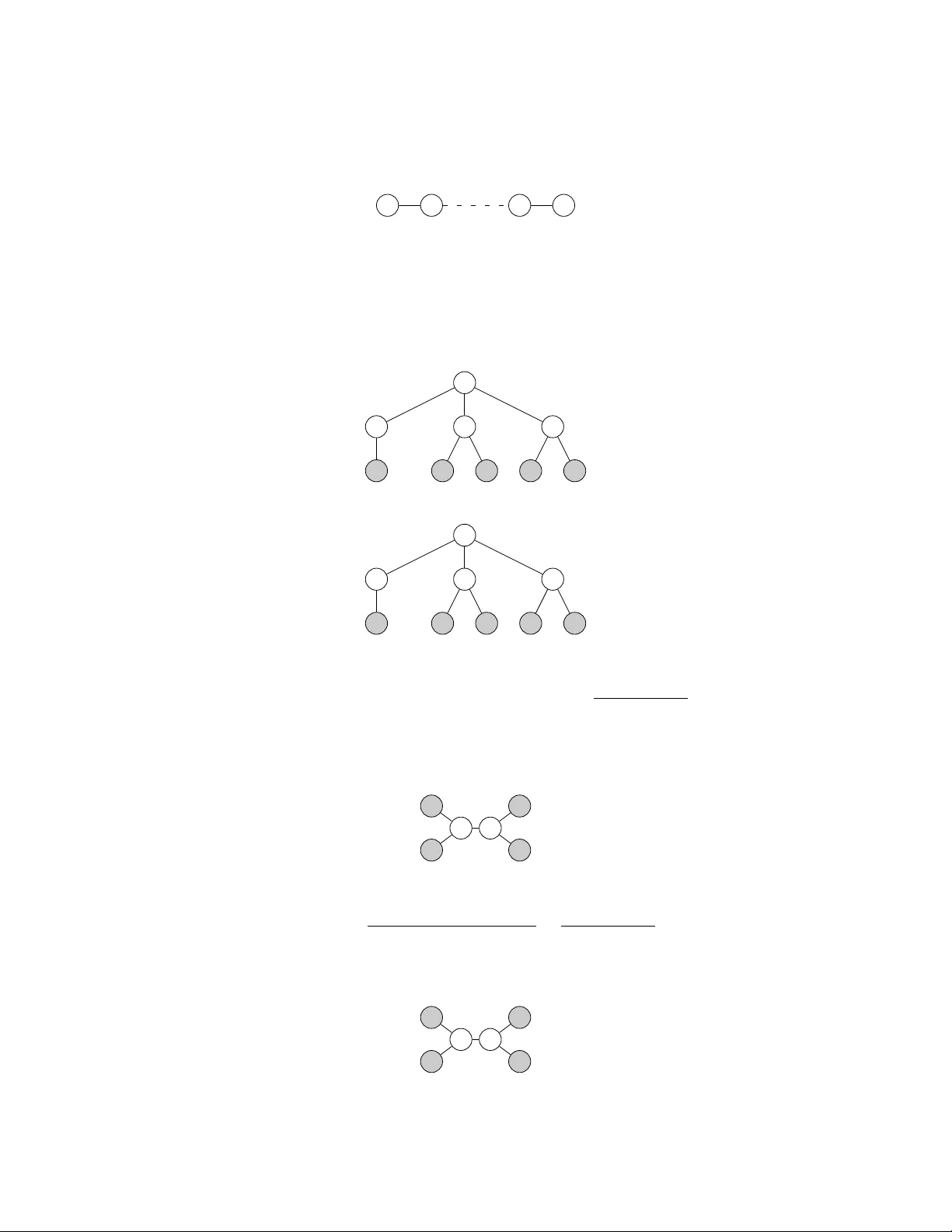
Sp ectral Metho ds for Learning Multiv ariate Laten t T ree Structure Animashree Anandkumar 1 , Kamalik a Chaudhuri 2 , Daniel Hsu 3 , Sham M. Kak ade 3,4 , Le Song 5 , and T ong Zhang 6 1 Departmen t of Electrical Engineering and Computer Science, UC Irvine 2 Departmen t of Computer Science and Engineering, UC San Diego 3 Microsoft Researc h New England 4 Departmen t of Statistics, Wharton School, Universit y of P ennsylv ania 5 Mac hine Learning Department, Carnegie Mellon Univ ersit y 6 Departmen t of Statistics, Rutgers Universit y Octob er 24, 2018 Abstract This w ork considers the problem of learning the structure of multiv ariate linear tree models, which include a v ariet y of directed tree graphical mo dels with con tinuous, discrete, and mixed laten t v ariables suc h as linear-Gaussian mo dels, hidden Marko v mo dels, Gaussian mixture mo dels, and Mark ov ev olu- tionary trees. The setting is one where we only hav e samples from certain observed v ariables in the tree, and our goal is to estimate the tree structure ( i.e. , the graph of how the underlying hidden v ariables are connected to each other and to the observed v ariables). W e prop ose the Sp ectral Recursive Grouping al- gorithm, an efficient and simple b ottom-up pro cedure for recov ering the tree structure from indep enden t samples of the observ ed v ariables. Our finite sample size b ounds for exact recov ery of the tree structure rev eal certain natural dep endencies on underlying statistical and structural prop erties of the underlying join t distribution. F urthermore, our sample complexity guarantees ha ve no explicit dependence on the dimensionalit y of the observed v ariables, making the algorithm applicable to many high-dimensional set- tings. A t the heart of our algorithm is a spectral quartet test for determining the relativ e top ology of a quartet of v ariables from second-order statistics. 1 In tro duction Graphical mo dels are a central to ol in modern mac hine learning applications, as they provide a natural metho dology for succinctly representing high-dimensional distributions. As suc h, they ha ve enjoy ed muc h success in v arious AI and machine learning applications such as natural language pro cessing, sp eec h recog- nition, rob otics, computer vision, and bioinformatics. The main statistical challenges asso ciated with graphical mo dels include estimation and inference. While the b ody of techniques for probabilistic inference in graphical mo dels is rather rich [29], current metho ds for tackling the more c hallenging problems of parameter and structure estimation are less developed and understo od, esp ecially in the presence of laten t (hidden) v ariables. The problem of parameter estimation in volv es determining the model parameters from samples of certain observ ed v ariables. Here, the predominant approac h is the exp ectation maximization (EM) algorithm, and only rather recently is the understanding of this algorithm improving [10, 5]. The problem of structure learning is to estimate the underlying graph E-mail: a.anandkumar@uci.edu , kamalika@cs.ucsd.edu , dahsu@microsoft.com , skakade@microsoft.com , lesong@cs.cmu.edu , tzhang@stat.rutgers.edu 1 z 1 z 2 z 3 z 4 h g z 1 z 3 z 2 z 4 h g z 1 z 4 z 2 z 3 h g z 1 z 4 z 2 z 3 h {{ z 1 , z 2 } , { z 3 , z 4 }} {{ z 1 , z 3 } , { z 2 , z 4 }} {{ z 1 , z 4 } , { z 2 , z 3 }} {{ z 1 , z 2 , z 3 , z 4 }} (a) (b) (c) (d) Figure 1: The four p ossible (undirected) tree top ologies ov er lea ves { z 1 , z 2 , z 3 , z 4 } . of the graphical mo del. In general, structure learning is NP-hard and becomes even more challenging when some v ariables are unobserved [6]. The main approac hes for structure estimation are either greedy or local searc h approaches [9, 15] or, more recen tly , based on conv ex relaxation [25]. This work fo cuses on learning the structure of multiv ariate latent tree graphical mo dels. Here, the underlying graph is a directed tree ( e.g. , hidden Marko v mo del, binary evolutionary tree), and only samples from a set of (multiv ariate) observed v ariables (the leav es of the tree) are av ailable for learning the structure. Laten t tree graphical mo dels are relev an t in many applications, ranging from computer vision, where one ma y learn ob ject/scene structure from the co-o ccurrences of ob jects to aid image understanding [7]; to ph ylogenetics, where the central task is to reconstruct the tree of life from the genetic material of surviving sp ecies [12]. Generally speaking, methods for learning laten t tree structure exploit structural prop erties afforded b y the tree that are rev ealed through certain statistical tests o ver ev ery c hoice of four v ariables in the tree. These quartet tests , which ha ve origins in structural equation mo deling [30, 3], are hypothesis tests of the relativ e configuration of four (possibly non-adjacent) no des/v ariables in the tree (see Figure 1); they are also related to the four p oint c ondition associated with a corresp onding additiv e tree metric induced by the distribution [4]. Some early metho ds for learning tree structure are based on the use of exact correlation statistics or distance measuremen ts ( e.g. , [24, 26]). Unfortunately , these metho ds ignore the crucial asp ect of estimation error, whic h ultimately gov erns their sample complexit y . Indeed, this (lac k of ) robustness to estimation error has b een quantified for v arious algorithms (notably , for the popular Neighbor Joining algorithm [14, 19]), and therefore serv es as a basis for comparing differen t methods. Subsequen t w ork in the area of mathematical ph ylogenetics has fo cused on the sample complexity of evolutionary tree reconstruction [13, 14, 20, 11]. The basic model there corresponds to a directed tree ov er discrete random v ariables, and muc h of the recent effort deals exclusively in the regime for a certain mo del parameter (the Kesten-Stigum regime [18]) that allows for a sample complexity that is p olylogarithmic in the num b er of lea v es, as opposed to p olynomial [20, 11]. Finally , recen t w ork in machine learning has developed structure learning metho ds for latent tree graphical models that extend b ey ond the discrete distributions of evolutionary trees [8], thereb y widening their applicabilit y to other problem domains. This work extends beyond previous studies, whic h hav e fo cused on laten t tree mo dels with either discrete or scalar Gaussian v ariables, by directly addressing the m ultiv ariate setting where hidden and observ ed no des ma y b e random v ectors rather than scalars. The generality of our tec hniques allo ws us to handle a muc h wider class of distributions than b efore, b oth in terms of the conditional indep endence properties imposed by the mo dels ( i.e. , the random vector asso ciated with a no de need not follow a distribution that corresp onds to a tree mo del), as well as other characteristics of the no de distributions ( e.g. , some no des in the tree could ha ve discrete state spaces and others con tinuous, as in a Gaussian mixture model). W e prop ose the Sp e ctr al R e cursive Gr ouping algorithm for learning multiv ariate latent tree structure. The algorithm has at its core a multiv ariate sp e ctr al quartet test , whic h extends the classical quartet tests for scalar v ariables b y applying spectral tec hniques from multiv ariate statistics (specifically canonical correlation analysis [2, 22]). Sp ectral metho ds ha ve enjo yed recen t success in the context of parameter estimation [21, 16, 27, 28]; our w ork shows that they are also useful for structure learning. W e use the sp ectral quartet test in a simple modification of the recursive grouping algorithm of [8] to perform the tree reconstruction. The algorithm is essen tially a robust method for reasoning about the results of quartet tests (view ed simply as h yp othesis tests); the tests either confirm or reject h yp otheses ab out the relative topology o ver quartets of 2 v ariables. By carefully choosing which tests to consider and prop erly in terpreting their results, the algorithm is able to reco ver the correct latent tree structure (with high probability) in a prov ably efficien t manner, in terms of b oth computational and sample complexit y . The recursive grouping pro cedure is similar to the short quartet metho d from ph ylogenetics [14], which also guarantees efficient reconstruction in the context of ev olutionary trees. How ev er, our metho d and analysis applies to considerably more general high-dimensional settings; for instance, our sample complexity bound is giv en in terms of natural correlation conditions that generalize the more restrictive effe ctive depth conditions of previous works [14, 8]. Finally , we note that while w e do not directly address the question of parameter estimation, pro v able parameter estimation metho ds ma y derived using the sp ectral tec hniques from [21, 16]. 2 Preliminaries 2.1 Laten t v ariable tree mo dels Let T b e a connected, directed tree graphical model with leav es V obs := { x 1 , x 2 , . . . , x n } and internal no des V hid := { h 1 , h 2 , . . . , h m } such that every no de has at most one paren t. The lea v es are termed the observe d variables and the internal no des hidden variables . Note that all no des in this work generally correspond to m ultiv ariate random v ectors; we will abuse terminology and still refer to these random vectors as random v ariables. F or any h ∈ V hid , let Children T ( h ) ⊆ V T denote the children of h in T . Eac h observ ed v ariable x ∈ V obs is mo deled as random v ector in R d , and eac h hidden v ariable h ∈ V hid as a random vector in R k . The joint distribution ov er all the v ariables V T := V obs ∪ V hid is assumed satisfy conditional independence properties specified b y the tree structure o v er the v ariables. Sp ecifically , for an y disjoin t subsets V 1 , V 2 , V 3 ⊆ V T suc h that V 3 separates V 1 from V 2 in T , the v ariables in V 1 are conditionally indep enden t of those in V 2 giv en V 3 . 2.2 Structural and distributional assumptions The class of mo dels considered are specified by the follo wing structural and distributional assumptions. Condition 1 (Linear conditional means) . Fix an y hidden v ariable h ∈ V hid . F or eac h hidden child g ∈ Children T ( h ) ∩ V hid , there exists a matrix A ( g | h ) ∈ R k × k suc h that E [ g | h ] = A ( g | h ) h ; and for each observed child x ∈ Children T ( h ) ∩ V obs , there exists a matrix C ( x | h ) ∈ R d × k suc h that E [ x | h ] = C ( x | h ) h. W e refer to the class of tree graphical mo dels satisfying Condition 1 as line ar tr e e mo dels . Such mo dels include a v ariet y of contin uous and discrete tree distributions (as well as h ybrid combinations of the t w o, suc h as Gaussian mixture mo dels) whic h are widely used in practice. Con tinuous linear tree models include linear-Gaussian models and Kalman filters. In the discrete case, suppose that the observed v ariables tak e on d v alues, and hidden v ariables tak e k v alues. Then, each v ariable is represen ted by a binary v ector in { 0 , 1 } s , where s = d for the observ ed v ariables and s = k for the hidden v ariables (in particular, if the v ariable takes v alue i , then the corresp onding vector is the i -th coordinate vector), and any conditional distribution b et ween the v ariables is represented b y a linear relationship. Thus, discrete linear tree mo dels include discrete hidden Marko v mo dels [16] and Marko vian evolutionary trees [21]. In addition to the linearit y , the follo wing conditions are assumed in order to recov er the hidden tree structure. F or any matrix M , let σ t ( M ) denote its t -th largest singular v alue. Condition 2 (Rank condition) . The v ariables in V T = V hid ∪ V obs ob ey the follo wing rank conditions. 1. F or all h ∈ V hid , E [ hh > ] has rank k ( i.e. , σ k ( E [ hh > ]) > 0). 3 x 6 x 1 x 2 x 3 h 1 h 2 x 4 x 5 h 3 h 4 T 1 T 2 T 3 Figure 2: Set of trees F h 4 = {T 1 , T 2 , T 3 } obtained if h 4 is remov ed. 2. F or all h ∈ V hid and hidden child g ∈ Children T ( h ) ∩ V hid , A ( g | h ) has rank k . 3. F or all h ∈ V hid and observed child x ∈ Children T ( h ) ∩ V obs , C ( x | h ) has rank k . The rank condition is a generalization of parameter identifiabilit y conditions in latent v ariable mo dels [1, 21, 16] which rules out v arious (prov ably) hard instances in discrete v ariable settings [21]. Condition 3 (Non-redundancy condition) . Each hidden v ariable has at least three neigh b ors. F urthermore, there exists ρ 2 max > 0 such that for eac h pair of distinct hidden v ariables h, g ∈ V hid , det( E [ hg > ]) 2 det( E [ hh > ]) det( E [ g g > ]) ≤ ρ 2 max < 1 . The requirement for eac h hidden no de to hav e three neighbors is natural; otherwise, the hidden node can be eliminated. The quantit y ρ max is a natural multiv ariate generalization of correlation. First, note that ρ max ≤ 1, and that if ρ max = 1 is achiev ed with some h and g , then h and g are completely correlated, implying the existence of a deterministic map b etw een hidden no des h and g ; hence simply merging the t wo no des into a single no de h (or g ) resolves this issue. Therefore the non-redundancy condition simply means that an y tw o hidden no des h and g cannot b e further reduced to a single node. Clearly , this condition is necessary for the goal of identifying the correct tree structure, and it is satisfied as so on as h and g hav e limited correlation in just a single direction. Previous w orks [24, 23] show that an analogous condition ensures identifiabilit y for gener al latent tree models (and in fact, the conditions are identical in the Gaussian case). Condition 3 is therefore a generalization of this condition suitable for the m ultiv ariate setting. Our learning guaran tees also require a correlation condition that generalize the explicit depth conditions considered in the phylogenetics literature [14, 21]. T o state this condition, first define F h to be the set of subtrees of that remain after a hidden v ariable h ∈ V hid is remov ed from T (see Figure 2). Also, for an y subtree T 0 of T , let V obs [ T 0 ] ⊆ V obs b e the observ ed v ariables in T 0 . Condition 4 (Correlation condition) . There exists γ min > 0 suc h that for all hidden v ariables h ∈ V hid and all triples of subtrees {T 1 , T 2 , T 3 } ⊆ F h in the forest obtained if h is remo ved from T , max x 1 ∈V obs [ T 1 ] ,x 2 ∈V obs [ T 2 ] ,x 3 ∈V obs [ T 3 ] min { i,j }⊂{ 1 , 2 , 3 } σ k ( E [ x i x > j ]) ≥ γ min . The quantit y γ min is related to the effe ctive depth of T , which is the maxim um graph distance b et ween a hidden v ariable and its closest observed v ariable [14, 8]. The effective depth is at most logarithmic in the n umber of v ariables (as achiev ed by a complete binary tree), though it can also b e a constant if every hidden v ariable is close to an observ ed v ariable ( e.g. , in a hidden Mark o v mo del, the effective depth is 1, even though the true depth, or diameter, is m + 1). If the matrices giving the (conditionally) linear relationship betw een neigh b oring v ariables in T are all w ell-conditioned, then γ min is at w orst exp onentially small in the effectiv e depth, and therefore at w orst p olynomially small in the num b er of v ariables. 4 Algorithm 1 Sp ectralQua rtetT est on observed v ariables { z 1 , z 2 , z 3 , z 4 } . Input: F or eac h pair { i, j } ⊂ { 1 , 2 , 3 , 4 } , an empirical estimate ˆ Σ i,j of the second-momen t matrix E [ z i z > j ] and a corresp onding confidence parameter ∆ i,j > 0. Output: Either a pairing {{ z i , z j } , { z i 0 , z j 0 }} or ⊥ . 1: if there exists a partition of { z 1 , z 2 , z 3 , z 4 } = { z i , z j } ∪ { z i 0 , z j 0 } such that k Y s =1 [ σ s ( ˆ Σ i,j ) − ∆ i,j ] + [ σ s ( ˆ Σ i 0 ,j 0 ) − ∆ i 0 ,j 0 ] + > k Y s =1 ( σ s ( ˆ Σ i 0 ,j ) + ∆ i 0 ,j )( σ s ( ˆ Σ i,j 0 ) + ∆ i,j 0 ) then return the pairing {{ z i , z j } , { z i 0 , z j 0 }} . 2: else return ⊥ . Finally , also define γ max := max { x 1 ,x 2 }⊆V obs { σ 1 ( E [ x 1 x > 2 ]) } to be the largest spectral norm of any second-momen t matrix b etw een observ ed v ariables. Note γ max ≤ 1 in the discrete case, and, in the con tinuous case, γ max ≤ 1 if each observed random v ector is in isotropic p osition. In this w ork, the Euclidean norm of a vector x is denoted by k x k , and the (induced) sp ectral norm of a matrix A is denoted b y k A k , i.e. , k A k := σ 1 ( A ) = sup {k Ax k : k x k = 1 } . 3 Sp ectral quartet tests This section describ es the core of our learning algorithm, a spectral quartet test that determines top ology of the subtree induced b y four observ ed v ariables { z 1 , z 2 , z 3 , z 4 } . There are four p ossibilities for the induced subtree, as sho wn in Figure 1. Our quartet test either returns the correct induced subtree among possibilities in Figure 1(a)–(c); or it outputs ⊥ to indicate abstinence. If the test returns ⊥ , then no guarantees are pro vided on the induced s ubtree topology . If it does return a subtree, then the output is guaran teed to be the correct induced subtree (with high probability). The quartet test proposed is describ ed in Algorithm 1 ( Sp ectralQua rtetT est ). The notation [ a ] + denotes max { 0 , a } and [ t ] (for an integer t ) denotes the set { 1 , 2 , . . . , t } . The quartet test is defined with resp ect to four observed v ariables Z := { z 1 , z 2 , z 3 , z 4 } . F or each pair of v ariables z i and z j , it tak es as input an empirical estimate ˆ Σ i,j of the second-moment matrix E [ z i z > j ], and confidence b ound parameters ∆ i,j whic h are functions of N , the num b er of samples used to compute the ˆ Σ i,j ’s, a confidence parameter δ , and of prop erties of the distributions of z i and z j . In practice, one uses a single threshold ∆ for all pairs, which is tuned b y the algorithm. Our theoretical analysis also applies to this case. The output of the test is either ⊥ or a p airing of the v ariables {{ z i , z j } , { z i 0 , z j 0 }} . F or example, if the output is the pairing is {{ z 1 , z 2 } , { z 3 , z 4 }} , then Figure 1(a) is the output topology . Ev en though the configuration in Figure 1(d) is a p ossibility , the sp ectral quartet test never returns {{ z 1 , z 2 , z 3 , z 4 }} , as there is no correct pairing of Z . The topology {{ z 1 , z 2 , z 3 , z 4 }} can b e viewed as a degenerate case of {{ z 1 , z 2 } , { z 3 , z 4 }} (sa y) where the hidden v ariables h and g are deterministically identical, and Condition 3 fails to hold with respect to h and g . 3.1 Prop erties of the sp ectral quartet test With exact second momen ts: The sp ectral quartet test is motiv ated b y the following lemma, whic h sho ws the relationship b et ween the singular v alues of second-momen t matrices of the z i ’s and the induced top ology among them in the latent tree. Let det k ( M ) := Q k s =1 σ s ( M ) denote the product of the k largest singular v alues of a matrix M . 5 Lemma 1 (Perfect quartet test) . Supp ose that the observe d variables Z = { z 1 , z 2 , z 3 , z 4 } have the true induc e d tr e e top olo gy shown in Figur e 1(a), and the tr e e mo del satisfies Condition 1 and Condition 2. Then det k ( E [ z 1 z > 3 ])det k ( E [ z 2 z > 4 ]) det k ( E [ z 1 z > 2 ])det k ( E [ z 3 z > 4 ]) = det k ( E [ z 1 z > 4 ])det k ( E [ z 2 z > 3 ]) det k ( E [ z 1 z > 2 ])det k ( E [ z 3 z > 4 ]) = det( E [ hg > ]) 2 det( E [ hh > ]) det( E [ g g > ]) ≤ 1 (1) and det k ( E [ z 1 z > 3 ])det k ( E [ z 2 z > 4 ]) = det k ( E [ z 1 z > 4 ])det k ( E [ z 2 z > 3 ]) . This lemma sho ws that given the true second-moment matrices and assuming Condition 3, the in- equalit y in (1) b ecomes strict and thus can b e used to deduce the correct top ology: the correct pairing is {{ z i , z j } , { z i 0 , z j 0 }} if and only if det k ( E [ z i z > j ])det k ( E [ z i 0 z > j 0 ]) > det k ( E [ z i 0 z > j ])det k ( E [ z i z > j 0 ]) . Reliabilit y: The next lemma shows that even if the singular v alues of E [ z i z > j ] are not known exactly , then with v alid confidence in terv als (that contain these singular v alues) a robust test can b e constructed which is reliable in the follo wing sense: if it do es not output ⊥ , then the output top ology is indeed the correct top ology . Lemma 2 (Reliability) . Consider the setup of L emma 1, and supp ose that Figur e 1(a) is the c orr e ct top olo gy. If for al l p airs { z i , z j } ⊂ Z and al l s ∈ [ k ] , σ s ( ˆ Σ i,j ) − ∆ i,j ≤ σ s ( E [ z i z > j ]) ≤ σ s ( ˆ Σ i,j ) + ∆ i,j , and if Sp ectralQua rtetT est r eturns a p airing {{ z i , z j } , { z i 0 , z j 0 }} , then {{ z i , z j } , { z i 0 , z j 0 }} = {{ z 1 , z 2 } , { z 3 , z 4 }} . In other words, the sp ectral quartet test never returns an incorrect pairing as long as the singular v alues of E [ z i z > j ] lie in an interv al of length 2∆ i,j around the singular v alues of ˆ Σ i,j . The lemma b elo w shows how to set the ∆ i,j s as a function of N , δ and prop erties of the distributions of z i and z j so that this required ev ent holds with probabilit y at least 1 − δ . W e remark that any v alid confidence interv als may b e used; the one described b elo w is particularly suitable when the observed v ariables are high-dimensional random v ectors. Lemma 3 (Confidence interv als) . L et Z = { z 1 , z 2 , z 3 , z 4 } b e four r andom ve ctors. L et k z i k ≤ M i almost sur ely, and let δ ∈ (0 , 1 / 6) . If e ach empiric al se c ond-moment matrix ˆ Σ i,j is c ompute d using N iid c opies of z i and z j , and if ¯ d i,j := E [ k z i k 2 k z j k 2 ] − tr( E [ z i z > j ] E [ z i z > j ] > ) max {k E [ k z j k 2 z i z > i ] k , k E [ k z i k 2 z j z > j ] k} , t i,j := 1 . 55 ln(24 ¯ d i,j /δ ) , ∆ i,j ≥ s 2 max    E [ k z j k 2 z i z > i ]   ,   E [ k z i k 2 z j z > j ]    t i,j N + M i M j t i,j 3 N , then with pr ob ability 1 − δ , for al l p airs { z i , z j } ⊂ Z and al l s ∈ [ k ] , σ s ( ˆ Σ i,j ) − ∆ i,j ≤ σ s ( E [ z i z > j ]) ≤ σ s ( ˆ Σ i,j ) + ∆ i,j . (2) Conditions for returning a correct pairing: The conditions under whic h Sp ectralQua rtetT est returns an induced top ology (as opp osed to ⊥ ) are now provided. An imp ortan t quantit y in this analysis is the level of non-redundancy b et ween the hidden v ariables h and g . Let ρ 2 := det( E [ hg > ]) 2 det( E [ hh > ]) det( E [ g g > ]) . (3) If Figure 1(a) is the correct induced topology among { z 1 , z 2 , z 3 , z 4 } , then the smaller ρ is, the greater the gap b et w een det k ( E [ z 1 z > 2 ])det k ( E [ z 3 z > 4 ]) and either of det k ( E [ z 1 z > 3 ])det k ( E [ z 2 z > 4 ]) and det k ( E [ z 1 z > 4 ])det k ( E [ z 2 z > 3 ]). Therefore, ρ also gov erns how small the ∆ i,j need to be for the quartet test to return a correct pairing; this is quantified in Lemma 4. Note that Condition 3 implies ρ ≤ ρ max < 1. 6 Lemma 4 (Correct pairing) . Supp ose that (i) the observe d variables Z = { z 1 , z 2 , z 3 , z 4 } have the true induc e d tr e e top olo gy shown in Figur e 1(a); (ii) the tr e e mo del satisfies Condition 1, Condition 2, and ρ < 1 (wher e ρ is define d in (3) ), and (iii) the c onfidenc e b ounds in (2) hold for al l { i, j } and al l s ∈ [ k ] . If ∆ i,j < 1 8 k · min n 1 , 1 ρ − 1 o · min { i,j } { σ k ( E [ z i z > j ]) } for e ach p air { i, j } , then Sp ectralQuartetT est r eturns the c orr e ct p airing {{ z 1 , z 2 } , { z 3 , z 4 }} . 4 The Sp ectral Recursiv e Grouping algorithm The Sp ectral Recursiv e Grouping algorithm, presented as Algorithm 2, uses the spectral quartet test dis- cussed in the previous section to estimate the structure of a m ultiv ariate latent tree distribution from iid samples of the observed leaf v ariables. 1 The algorithm is a modification of the recursive grouping (R G) pro cedure prop osed in [8]. R G builds the tree in a b ottom-up fashion, where the initial working set of v ariables are the observed v ariables. The v ariables in the working set alwa ys correspond to roots of disjoin t subtrees of T disco vered by the algorithm. (Note that b ecause these subtrees are rooted, they naturally induce parent/c hild relationships, but these may differ from those implied by the edge directions in T .) In eac h iteration, the algorithm determines which v ariables in the w orking set to combine. If the v ariables are com bined as siblings, then a new hidden v ariable is in tro duced as their paren t and is added to the working set, and its c hildren are remov ed. If the v ariables are combined as neighbors (parent/c hild), then the child is remov ed from the working set. The pro cess repeats until the en tire tree is constructed. Our modification of R G uses the sp ectral quartet tests from Section 3 to decide which subtree ro ots in the curren t working set to combine. Note that b ecause the test ma y return ⊥ (a null result), our algorithm uses the tests to rule out p ossible siblings or neighbors among v ariables in the working set—this is encapsulated in the subroutine Mergeable (Algorithm 3), whic h tests quartets of observed v ariables (lea v es) in the subtrees ro oted at w orking set v ariables. F or any pair { u, v } ⊆ R submitted to the subroutine (along with the curren t w orking set R and leaf sets L [ · ]): • Mergeable returns false if there is evidence (provided by a quartet test) that u and v should first be joined with different v ariables ( u 0 and v 0 , resp ectively) b efore joining with eac h other; and • Mergeable returns true if no quartet test provides such evidence. The subroutine is also used by the subroutine Relationship (Algorithm 4) which determines whether a can- didate pair of v ariables should b e merged as neigh b ors (paren t/child) or as siblings: essentially , to chec k if u is a parent of v , it chec ks if v is a sibling of each child of u . The use of unreliable estimates of long-range correlations is a voided b y only considering highly-correlated v ariables as candidate pairs to merge (where correlation is measured using observed v ariables in their corresponding subtrees as proxies). This leads to a sample-efficien t algorithm for recov ering the hidden tree structure. The Sp ectral Recursiv e Grouping algorithm enjoys the following guaran tee. Theorem 1. L et η ∈ (0 , 1) . Assume the dir e cte d tr e e gr aphic al mo del T over variables (r andom ve ctors) V T = V obs ∪ V hid satisfies Conditions 1, 2, 3, and 4. Supp ose the Sp e ctr al R e cursive Gr ouping algorithm (A lgorithm 2) is pr ovide d N indep endent samples fr om the distribution over V obs , and uses p ar ameters given by ∆ x i ,x j := r 2 B x i ,x j t x i ,x j N + M x i M x j t x i ,x j 3 N (4) 1 T o simplify notation, we assume that the estimated second-moment matrices b Σ x,y and threshold parameters ∆ x,y ≥ 0 for all pairs { x, y } ⊂ V obs are globally defined. In particular, we assume the sp ectral quartet tests use these quantities. 7 Algorithm 2 Sp ectral Recursive Grouping. Input: Empirical second-moment matrices b Σ x,y for all pairs { x, y } ⊂ V obs computed from N iid samples from the distribution ov er V obs ; threshold parameters ∆ x,y for all pairs { x, y } ⊂ V obs . Output: T ree structure b T or “failure”. 1: let R := V obs , and for all x ∈ R , T [ x ] := ro oted single-node tree x and L [ x ] := { x } . 2: while |R| > 1 do 3: let pair { u, v } ∈ {{ ˜ u, ˜ v } ⊆ R : Mergeable ( R , L [ · ] , ˜ u, ˜ v ) = true } be suc h that max { σ k ( b Σ x,y ) : ( x, y ) ∈ L [ u ] × L [ v ] } is maximized. If no such pair exists, then halt and return “failure”. 4: let result := Relationship ( R , L [ · ] , T [ · ] , u, v ). 5: if result = “siblings” then 6: Create a new v ariable h , create subtree T [ h ] ro oted at h by joining T [ u ] and T [ v ] to h with edges { h, u } and { h, v } , and set L [ h ] := L [ u ] ∪ L [ v ]. 7: Add h to R , and remov e u and v from R . 8: else if result = “ u is parent of v ” then 9: Mo dify subtree T [ u ] by joining T [ v ] to u with an edge { u, v } , and mo dify L [ u ] := L [ u ] ∪ L [ v ]. 10: Remo ve v from R . 11: else if result = “ v is paren t of u ” then 12: { Analogous to ab o ve case. } 13: end if 14: end while 15: Return b T := T [ h ] where R = { h } . Algorithm 3 Subroutine Mergeable ( R , L [ · ] , u, v ). Input: Set of no des R ; leaf sets L [ v ] for all v ∈ R ; distinct u, v ∈ R . Output: true or false. 1: if there exists distinct u 0 , v 0 ∈ R \ { u, v } and ( x, y , x 0 , y 0 ) ∈ L [ u ] × L [ v ] × L [ u 0 ] × L [ v 0 ] s.t. Sp ectralQua rtetT est ( { x, y , x 0 , y 0 } ) returns {{ x, x 0 } , { y , y 0 }} or {{ x, y 0 } , { x 0 , y }} then return false. 2: else return true. wher e B x i ,x j := max    E [ k x i k 2 x j x > j ]   ,   E [ k x j k 2 x i x > i ]    , M x i ≥ k x i k almost sur ely , ¯ d x i ,x j := E [ k x i k 2 k x j k 2 ] − tr( E [ x i x > j ] E [ x j x > i ]) max    E [ k x j k 2 x i x > i ]   ,   E [ k x i k 2 x j x > j ]    , t x i ,x j := 4 ln(4 ¯ d x i ,x j n/η ) . L et B := max x i ,x j ∈V obs { B x i ,x j } , M := max x i ∈V obs { M x i } , t := max x i ,x j ∈V obs { t x i ,x j } . If N > 200 · k 2 · B · t  γ 2 min γ max · (1 − ρ max )  2 + 7 · k · M 2 · t γ 2 min γ max · (1 − ρ max ) , then with pr ob ability at le ast 1 − η , the Sp e ctr al R e cursive Gr ouping algorithm r eturns a tr e e b T with the same undir e cte d gr aph structur e as T . Consistency is implied b y the ab o ve theorem with an appropriate scaling of η with N . The theorem rev eals that the sample complexity of the algorithm dep ends solely on in trinsic sp ectral prop erties of the distribution. Note that there is no explicit dep endence on the dimensions of the observ able v ariables, which mak es the result applicable to high-dimensional settings. 8 Algorithm 4 Subroutine Relationship ( R , L [ · ] , T [ · ] , u, v ). Input: Set of no des R ; leaf sets L [ v ] for all v ∈ R ; ro oted subtrees T [ v ] for all v ∈ R ; distinct u, v ∈ R . Output: “siblings”, “ u is parent of v ” (“ u → v ”), or “ v is parent of u ” (“ v → u ”). 1: if u is a leaf then assert u 6→ v . 2: if v is a leaf then assert v 6→ u . 3: let R [ w ] := ( R \ { w } ) ∪ { w 0 : w 0 is a child of w in T [ w ] } for eac h w ∈ { u, v } . 4: if there exists child u 1 of u in T [ u ] s.t. Mergeable ( R [ u ] , L [ · ] , u 1 , v ) = false then assert “ u 6→ v ”. 5: if there exists child v 1 of v in T [ v ] s.t. Mergeable ( R [ v ] , L [ · ] , u, v 1 ) = false then assert “ v 6→ u ”. 6: if b oth “ u 6→ v ” and “ v 6→ u ” were asserted then return “siblings”. 7: else if “ u 6→ v ” was asserted then return “ v is parent of u ” (“ v → u ”). 8: else return “ u is paren t of v ” (“ u → v ”). Ac knowledgemen ts P art of this work was completed while DH w as at the Wharton School of the Univ ersity of Pennsylv ania and at Rutgers Univ ersity . AA was supp orted by in part by the setup funds at UCI and the AFOSR Award F A9550-10-1-0310. References [1] E. S. Allman, C. Matias, and J. A. Rho des. Iden tifiability of parameters in latent structure models with many observ ed v ariables. The Annals of Statistics , 37(6A):3099–3132, 2009. [2] M. S. Bartlett. F urther asp ects of the theory of multiple regression. Mathematic al Pr o c e e dings of the Cambridge Philosophic al So ciety , 34:33–40, 1938. [3] K. Bollen. Structur al Equation Mo dels with L atent V ariables . John Wiley & Sons, 1989. [4] P . Buneman. The reco v ery of trees from measuremen ts of dissimilarity . In F. R. Hodson, D. G. Kendall, and P . T autu, editors, Mathematics in the Ar chae olo gic al and Historic al Scienc es , pages 387–395. 1971. [5] K. Chaudhuri, S. Dasgupta, and A. V attani. Learning mixtures of Gaussians using the k -means algorithm, 2009. [6] D. M. Chick ering, D. Heck erman, and C. Meek. Large-sample learning of Ba yesian net works is NP-hard. Journal of Machine L e arning R ese ar ch , 5:1287–1330, 2004. [7] M. J. Choi, J. J. Lim, A. T orralba, and A. S. Willsky . Exploiting hierarchical context on a large database of ob ject categories. In IEEE Confer enc e on Computer Vision and Pattern R e c o gnition , 2010. [8] M. J. Choi, V. T an, A. Anandkumar, and A. Willsky . Learning latent tree graphical models. Journal of Machine L e arning R ese ar ch , 12:1771–1812, 2011. [9] C. Cho w and C. Liu. Approximating discrete probabilit y distributions with dep endence trees. IEEE T r ansactions on Information The ory , 14(3):462–467, 1968. [10] S. Dasgupta and L. Sch ulman. A probabilistic analysis of EM for mixtures of separated, spherical Gaussians. Journal of Machine L e arning R ese ar ch , 8(F eb):203–226, 2007. [11] C. Dask alakis, E. Mossel, and S. Ro c h. Evolutionary trees and the Ising mo del on the Bethe lattice: A pro of of Steel’s conjecture. Pr ob ability The ory and R elate d Fields , 149(1–2):149–189, 2011. [12] R. Durbin, S. R. Eddy , A. Krogh, and G. Mitchison. Biolo gic al Se quenc e Analysis: Pr ob abilistic Mo dels of Pr oteins and Nucleic A cids . Cambridge Universit y Press, 1999. [13] P . L. Erd¨ os, L. A. Sz ´ ekely , M. A. Steel, and T. J. W arnow. A few logs suffice to build (almost) all trees (I). R andom Structur es and A lgorithms , 14:153–184, 1999. [14] P . L. Erd¨ os, L. A. Sz´ ek ely , M. A. Steel, and T. J. W arnow. A few logs suffice to build (almost) all trees: Part I I. The or etic al Computer Scienc e , 221:77–118, 1999. [15] N. F riedman, I. Nachman, and D. Pe ´ er. Learning Ba yesian net work structure from massiv e datasets: the “sparse candidate” algorithm. In Fifte enth Confer enc e on Unc ertainty in Artificial Intel ligenc e , 1999. 9 [16] D. Hsu, S. M. Kak ade, and T. Zhang. A spectral algorithm for learning hidden Mark ov mo dels. In Twenty-Se c ond Annual Conferenc e on L e arning The ory , 2009. [17] D. Hsu, S. M. Kak ade, and T. Zhang. Dimension-free tail inequalities for sums of random matrices, 2011. [18] H. Kesten and B. P . Stigum. Additional limit theorems for indecomp osable multidimensional galton-w atson pro cesses. Annals of Mathematic al Statistics , 37:1463–1481, 1966. [19] M. R. Lacey and J. T. Chang. A signal-to-noise analysis of phylogen y estimation by neighbor-joining: insuffi- ciency of p olynomial length sequences. Mathematical Biosciences , 199(2):188–215, 2006. [20] E. Mossel. Phase transitions in phylogen y . T r ansactions of the Americ an Mathematic al So ciety , 356(6):2379– 2404, 2004. [21] E. Mossel and S. Roch. Learning nonsingular phylogenies and hidden Mark ov mo dels. Annals of Applied Pr ob ability , 16(2):583–614, 2006. [22] R. J. Muirhead and C. M. W aternaux. Asymptotic distributions in canonical correlation analysis and other m ultiv ariate pro cedures for nonnormal p opulations. Biometrika , 67(1):31–43, 1980. [23] J. Pearl. Pr ob abilistic R e asoning in Intel ligent Systems—Networks of Plausible Infer ence . Morgan Kaufmann, 1988. [24] J. Pearl and M. T arsi. Structuring causal trees. Journal of Complexity , 2(1):60–77, 1986. [25] P . Ravikumar, M. J. W ainwrigh t, and J. Lafferty . High-dimensional Ising mo del selection using ` 1 -regularized logistic regression. Annals of Statistics , 38(3):1287–1319, 2010. [26] N. Saitou and M. Nei. The neighbor-joining metho d: A new metho d for reconstructing phylogenetic trees. Mole cular Biolo gy and Evolution , 4:406–425, 1987. [27] S. M. Siddiqi, B. Bo ots, and G. J. Gordon. Reduced-rank hidden Marko v mo dels. In Thirte enth International Confer enc e on Artificial Intel ligenc e and Statistics , 2010. [28] L. Song, S. M. Siddiqi, G. J. Gordon, and A. J. Smola. Hilb ert space embeddings of hidden Marko v mo dels. In International Confer enc e on Machine L e arning , 2010. [29] M. J. W ain wright and M. I. Jordan. Graphical mo dels, exp onen tial families, and v ariational inference. F ounda- tions and T r ends in Machine L e arning , 1(1-2):1–305, 2008. [30] J. Wishart. Sampling errors in the theory of tw o factors. British Journal of Psycholo gy , 19:180–187, 1928. A Sample-based confidence in terv als for singular v alues W e sho w ho w to deriv e confidence b ounds for the singular v alues of Σ i,j := E [ z i z > j ] for { i, j } ⊂ { 1 , 2 , 3 , 4 } from N iid copies of the random vectors { z 1 , z 2 , z 3 , z 4 } . That is, we show how to set ∆ i,j so that, with high probabilit y , σ s ( ˆ Σ i,j ) − ∆ i,j ≤ σ s ( Σ i,j ) ≤ σ s ( ˆ Σ i,j ) + ∆ i,j for all { i, j } and all s ∈ [ k ]. W e state exp onen tial tail inequalities for the sp ectral norm of the estimation error ˆ Σ i,j − Σ i,j . The first exp onen tial tail inequality is stated for general random v ectors under Bernstein-type conditions, and the second is sp ecific to random v ectors in the discrete setting. Lemma 5. L et z i and z j b e r andom ve ctors such that k z i k ≤ M i and k z j k ≤ M j almost sur ely, and let ¯ d i,j := E [ k z i k 2 k z j k 2 ] − tr( Σ i,j Σ > i,j ) max    E [ k z j k 2 z i z > i ]   ,   E [ k z i k 2 z j z > j ]    ≤ max { dim( z i ) , dim( z j ) } . L et Σ i,j := E [ z i z > j ] and let ˆ Σ i,j b e the empiric al aver age of N indep endent c opies of z i z > j . Pick any t > 0 . With pr ob ability at le ast 1 − 4 ¯ d i,j t ( e t − t − 1) − 1 ,    ˆ Σ i,j − Σ i,j    ≤ s 2 max    E [ k z j k 2 z i z > i ]   ,   E [ k z i k 2 z j z > j ]    t N + M i M j t 3 N . 10 R emark 1 . F or an y δ ∈ (0 , 1 / 6), w e hav e 4 ¯ d i,j t ( e t − t − 1) − 1 ≤ δ pro vided that t ≥ 1 . 55 ln(4 ¯ d i,j /δ ). Pr o of. Define the random matrix Z :=  z i z > j z j z > i  . Let Z 1 , . . . , Z N b e indep enden t copies of Z . Then Pr h    ˆ Σ i,j − Σ i,j    > t i = Pr "     1 N N X ` =1 Z ` − E [ Z ]     > t # . Note that E [ Z 2 ] = E  k z j k 2 z i z > i k z i k 2 z j z > j  so by conv exity ,   E [ Z 2 ] − E [ Z ] 2   ≤   E [ Z 2 ]   ≤ max    E [ k z j k 2 z i z > i ]   ,   E [ k z i k 2 z j z > j ]    and tr( E [ Z 2 ] − E [ Z ] 2 ) = tr( E [ k z j k 2 z i z > i ]) + tr( E [ k z i k 2 z j z > j ]) − tr( Σ i,j Σ > i,j ) − tr( Σ > i,j Σ i,j ) = 2  E [ k z i k 2 k z j k 2 ] − tr( Σ i,j Σ > i,j )  . Moreo ver, k Z k ≤ k z i kk z j k ≤ M i M j . By the matrix Bernstein inequalit y [17], for any t > 0, Pr      ˆ Σ i,j − Σ i,j    > s 2  max    E [ k z j k 2 z i z > i ]   ,   E [ k z i k 2 z j z > j ]    t N + M i M j t 3 N   ≤ 2 · 2  E [ k z i k 2 k z j k 2 ] − tr( Σ i,j Σ > i,j )  max    E [ k z j k 2 z i z > i ]   ,   E [ k z i k 2 z j z > j ]    · t ( e t − t − 1) − 1 = 4 ¯ d i,j t ( e t − t − 1) − 1 . The claim follows. In the case of discrete random v ariables (modeled as random vectors as described in Section 2), the follo wing lemma from [16] can giv e a tigh ter exp onen tial tail inequality . Lemma 6 ([16]) . L et z i and z j b e r andom ve ctors, e ach with supp ort on the vertic es of a pr ob ability simplex. L et Σ i,j := E [ z i z > j ] and let ˆ Σ i,j b e the empiric al aver age of N indep endent c opies of z i z > j . Pick any t > 0 . With pr ob ability at le ast 1 − e − t ,    ˆ Σ i,j − Σ i,j    ≤    ˆ Σ i,j − Σ i,j    F ≤ 1 + √ t √ N (wher e k A k F denotes the F r ob enius norm of a matrix A ). F or simplicity , we only work with Lemma 5, although it is easy to translate all of our results by changing the tail inequality . The pro of of Lemma 3 is immediate from combining Lemma 5 and W eyl’s Theorem. 11 Lemma 3 provides some guidelines on how to set the ∆ i,j as functions of N , δ , and properties of z i and z j . The dep endence on the properties of z i and z j comes through the quantities M i , M j , ¯ d i,j , and B i,j := max i,j {   E [ k z j k 2 z i z > i ]   ,   E [ k z i k 2 z j z > j ]   } . In practice, one may use plug-in estimates for these quantities, or use lo ose upper b ounds based on weak er kno wledge of the distribution. F or instance, ¯ d i,j is at most max { dim( z i ) , dim( z j ) } , the larger of the explicit v ector dimensions of z i and z j . Also, if the maximum directional standard deviation σ ∗ of an y z i is kno wn, then B i,j ≤ max { M 2 i , M 2 j } σ 2 ∗ . W e note that as these are additiv e confidence in terv als, some dep endence on the prop erties of z i and z j is inevitable. B Analysis of the sp ectral quartet test F or any hidden v ariable h ∈ V hid , let Descendan ts T ( h ) ⊆ V T b e the descendan ts of h in T . F or any g ∈ Descendan ts T ( h ) ∩ V hid suc h that the (directed) path from h to g is h → g 1 → g 2 → · · · → g q = g , define A ( g | h ) ∈ R k × k to b e the pro duct A ( g | h ) := A ( g q | g q − 1 ) · · · A ( g 2 | g 1 ) A ( g 1 | h ) . Similarly , for any x ∈ Descendants T ( h ) ∩ V obs suc h that the (directed) path from h to x is h → g 1 → g 2 → · · · → g q → x , define C ( x | h ) ∈ R d × k to b e the pro duct C ( x | h ) := C ( x | g q ) A ( g q | g q − 1 ) · · · A ( g 2 | g 1 ) A ( g 1 | h ) . B.1 log det k metric Define the function µ : V T × V T → R by µ ( u, v ) :=          log det k ( E [ uu > ] − 1 / 2 E [ uv > ] E [ v v > ] − 1 / 2 ) if u, v ∈ V hid log det k ( E [ uv > ] E [ v v > ] − 1 / 2 ) if u ∈ V obs , v ∈ V hid log det k ( E [ uu > ] − 1 / 2 E [ uv > ]) if u ∈ V hid , v ∈ V obs log det k ( E [ uv > ]) if u, v ∈ V obs . Prop osition 1 (log det k metric) . Assume Conditions 1 and 2 hold, and pick any u, v ∈ V T . If w ∈ V T \ { u, v } is on the (undir e cte d) p ath u v , then µ ( u, v ) = µ ( u, w ) + µ ( w , v ) . Pr o of. Supp ose the induced top ology ov er u, v , w in T is the following. u w v Assume for now that u, v ∈ V hid . Then, using Condition 1, E [ uv > ] = E [ uw > ] A > ( v | w ) = ( E [ uw > ] E [ w w > ] − 1 / 2 )( E [ w w > ] − 1 / 2 E [ w v > ]) so, b ecause rank( E [ uu > ] − 1 / 2 E [ uw > ] E [ w w > ] − 1 / 2 ) = rank( E [ w w > ] − 1 / 2 E [ w v > ] E [ v v > ] − 1 / 2 ) = k by Condi- tion 2, µ ( u, v ) = log det k ( E [ uu > ] − 1 / 2 E [ uw > ] E [ w w > ] − 1 / 2 E [ w w > ] − 1 / 2 E [ w v > ] E [ v v > ] − 1 / 2 ) = log det k ( E [ uu > ] − 1 / 2 E [ uw > ] E [ w w > ] − 1 / 2 ) + log det k ( E [ w w > ] − 1 / 2 E [ w v > ] E [ v v > ] − 1 / 2 ) = µ ( u, w ) + µ ( w , v ) . 12 If u ∈ V hid but v ∈ V obs , then let U v ∈ R d × k b e a matrix of orthonormal left singular vectors of C ( v | w ) . Then E [ uv > ] = ( E [ uw > ] E [ w w > ] − 1 / 2 )( E [ w w > ] − 1 / 2 E [ w v > ]) as b efore, and det k ( E [ uu > ] − 1 / 2 E [ uv > ]) = | det( E [ uu > ] − 1 / 2 E [ uv > ] U v ) | = | det( E [ uu > ] − 1 / 2 ) | · | det( E [ uv > ] U v ) | = det k ( E [ uu > ] − 1 / 2 E [ uw > ] E [ w w > ] − 1 / 2 ) · det k ( E [ w w > ] − 1 / 2 E [ w v > ] U v ) = det k ( E [ uu > ] − 1 / 2 E [ uw > ] E [ w w > ] − 1 / 2 ) · det k ( E [ w w > ] − 1 / 2 E [ w v > ]) , so µ ( u, v ) = log det k ( E [ uu > ] − 1 / 2 E [ uw > ] E [ w w > ] − 1 / 2 ) + log det k ( E [ w w > ] − 1 / 2 E [ w v > ]) = µ ( u, w ) + µ ( w , v ) . Supp ose now that the induced toplogy o ver u, v , w in T is the following. u w v Again, first assume that u, v ∈ V hid . Then, by Condition 1, E [ uv > ] = A ( u | w ) E [ w w > ] A > ( v | w ) = ( E [ uw > ] E [ w w > ] − 1 / 2 )( E [ w w > ] − 1 / 2 E [ w v > ]) , so µ ( u, v ) = µ ( u, w ) + µ ( v , w ) as before. The cases where one or b oth of u and v is in V obs follo w b y similar argumen ts as abov e. B.2 Pro of of Lemma 1 By Prop osition 1, det k ( E [ z 1 z > 3 ]) · det k ( E [ z 2 z > 4 ]) = exp( µ ( z 1 , z 3 ) + µ ( z 2 , z 4 )) = exp( µ ( z 1 , h ) + µ ( h, g ) + µ ( g , z 3 ) + µ ( z 2 , h ) + µ ( h, g ) + µ ( g , z 4 )) = exp( µ ( z 1 , h ) + µ ( h, g ) + µ ( g , z 4 ) + µ ( z 2 , h ) + µ ( h, g ) + µ ( g , z 3 )) = exp( µ ( z 1 , z 4 ) + µ ( z 2 , z 3 )) = det k ( E [ z 1 z > 4 ]) · det k ( E [ z 2 z > 3 ]) . Moreo ver, det k ( E [ z 1 z > 3 ]) · det k ( E [ z 2 z > 4 ]) det k ( E [ z 1 z > 2 ]) · det k ( E [ z 3 z > 4 ]) = exp( µ ( z 1 , z 3 ) + µ ( z 2 , z 4 )) exp( µ ( z 1 , z 2 ) + µ ( z 3 , z 4 )) = exp( µ ( z 1 , h ) + µ ( h, g ) + µ ( g , z 3 ) + µ ( z 2 , h ) + µ ( h, g ) + µ ( g , z 4 )) exp( µ ( z 1 , h ) + µ ( h, z 2 ) + µ ( z 3 , g ) + µ ( g , z 4 )) = exp(2 µ ( h, g )) = det( E [ hh > ] − 1 / 2 E [ hg > ] E [ g g > ] − 1 / 2 ) 2 = det( E [ hg > ]) 2 det( E [ hh > ]) · det( E [ g g > ]) . Finally , note that u > E [ hh > ] − 1 / 2 E [ hg > ] E [ g g > ] − 1 / 2 v ≤ k u kk v k for all vectors u and v by Cauch y-Sch w arz, so det( E [ hg > ]) 2 det( E [ hh > ]) · det( E [ g g > ]) = det( E [ hh > ] − 1 / 2 E [ hg > ] E [ g g > ] − 1 / 2 ) 2 ≤ 1 as required. Note that if Condition 3 also holds, then Lemma 1 implies the strict inequalities max  det k ( E [ z 1 z > 3 ]) · det k ( E [ z 2 z > 4 ]) , det k ( E [ z 1 z > 4 ]) · det k ( E [ z 2 z > 3 ])  < det k ( E [ z 1 z > 2 ]) · det k ( E [ z 3 z > 4 ]) . 13 B.3 Pro of of Lemma 2 Giv en that (2) holds for all pairs { i, j } and all s ∈ { 1 , 2 , . . . , k } , if the sp ectral quartet test returns a pairing {{ z i , z j } , { z i 0 , z j 0 }} , it must b e that k Y s =1 σ s ( E [ z i z > j ]) σ s ( E [ z i 0 z > j 0 ]) ≥ k Y s =1 [ σ s ( ˆ Σ i,j ) − ∆ i,j ] + [ σ s ( ˆ Σ i 0 ,j 0 ) − ∆ i 0 ,j 0 ] + > k Y s =1 ( σ s ( ˆ Σ i 0 ,j ) + ∆ i 0 ,j )( σ s ( ˆ Σ i,j 0 ) + ∆ i,j 0 ) ≥ k Y s =1 σ s ( E [ z i 0 z > j ]) σ s ( E [ z i z > j 0 ]) . Therefore det k ( E [ z i z > j ]) · det k ( E [ z i 0 z > j 0 ]) = k Y s =1 σ s ( E [ z i z > j ]) σ s ( E [ z i 0 z > j 0 ]) > k Y s =1 σ s ( E [ z i 0 z > j ]) σ s ( E [ z i z > j 0 ]) = det k ( E [ z i 0 z > j ]) · det k ( E [ z i z > j 0 ]) . But by Lemma 1, the abov e inequalit y can only hold if {{ z i , z j } , { z i 0 , z j 0 }} = {{ z 1 , z 2 } , { z 3 , z 4 }} . B.4 Pro of of Lemma 4 Let Σ i,j := E [ z i z > j ]. The assumptions in the statement of the lemma imply max { ∆ 1 , 2 , ∆ 3 , 4 } <  0 8 k min { σ k ( Σ 1 , 2 ) , σ k ( Σ 3 , 4 ) } where  0 := min n 1 ρ − 1 , 1 o . Therefore k Y s =1 [ σ s ( ˆ Σ 1 , 2 ) − ∆ 1 , 2 ] + [ σ s ( ˆ Σ 3 , 4 ) − ∆ 3 , 4 ] + ≥ k Y s =1 [ σ s ( Σ 1 , 2 ) − 2∆ 1 , 2 ] + [ σ s ( Σ 3 , 4 ) − 2∆ 3 , 4 ] + > k Y s =1 σ s ( Σ 1 , 2 ) σ s ( Σ 3 , 4 ) !  1 −  0 4 k  2 k ≥ k Y s =1 σ s ( Σ 1 , 2 ) σ s ( Σ 3 , 4 ) ! (1 −  0 / 2) . (5) If E [ hg > ] has rank k , then so do Σ i,j for i ∈ { 1 , 2 } and j ∈ { 3 , 4 } . Therefore, for { i 0 , j 0 } = { 1 , 2 , 3 , 4 } \ { i, j } , max { ∆ i,j , ∆ i 0 ,j 0 } <  0 8 k min { σ k ( Σ i 0 ,j 0 ) , σ k ( Σ i 0 ,j 0 ) } . This implies k Y s =1 ( σ s ( ˆ Σ i,j ) + ∆ i,j )( σ s ( ˆ Σ i 0 ,j 0 ) + ∆ i 0 ,j 0 ) ≤ k Y s =1 ( σ s ( Σ i,j ) + 2∆ i,j )( σ s ( Σ i 0 ,j 0 ) + 2∆ i 0 ,j 0 ) < k Y s =1 σ s ( Σ i,j ) σ s ( Σ i 0 ,j 0 ) !  1 +  0 4 k  2 k ≤ k Y s =1 σ s ( Σ i,j ) σ s ( Σ i 0 ,j 0 ) ! (1 +  0 ) . (6) 14 Therefore, combining (5), (6), and Lemma 1, k Y s =1 [ σ s ( ˆ Σ 1 , 2 ) − ∆ 1 , 2 ] + [ σ s ( ˆ Σ 3 , 4 ) − ∆ 3 , 4 ] + > 1 −  0 / 2 1 +  0 · det( E [ hh > ]) det( E [ g g > ]) det( E [ hg > ]) 2 · k Y s =1 ( σ s ( ˆ Σ i,j ) + ∆ i,j )( σ s ( ˆ Σ i 0 ,j 0 ) + ∆ i 0 ,j 0 ) ≥ 1 (1 +  0 ) 2 · det( E [ hh > ]) det( E [ g g > ]) det( E [ hg > ]) 2 · k Y s =1 ( σ s ( ˆ Σ i,j ) + ∆ i,j )( σ s ( ˆ Σ i 0 ,j 0 ) + ∆ i 0 ,j 0 ) ≥ k Y s =1 ( σ s ( ˆ Σ i,j ) + ∆ i,j )( σ s ( ˆ Σ i 0 ,j 0 ) + ∆ i 0 ,j 0 ) , so the sp ectral quartet test will return the correct pairing {{ z 1 , z 2 } , { z 3 , z 4 }} , proving the lemma. B.5 Conditions for returning a correct pairing when rank( E [ hg > ]) < k The spectral quartet test is also useful in the case where E [ hg > ] has rank r < k . In this case, the widths of the confidence interv als are allo wed to b e wider than in the case where rank( E [ hg > ]) = k . Define σ min := min  { σ k ( Σ 1 , 2 ) , σ k ( Σ 3 , 4 ) } ∪ { σ r ( Σ i,j ) : i ∈ { 1 , 2 } , j ∈ { 3 , 4 }}  . ρ 2 1 = σ 2( k − r ) min · max i,j,i 0 ,j 0 Q r s =1 σ s ( Σ i,j ) σ s ( Σ i 0 ,j 0 ) Q k s =1 σ s ( Σ 1 , 2 ) σ s ( Σ 3 , 4 ) . Instead of dep ending on min i,j { σ k ( Σ i,j ) } and ρ as in the case where rank( E [ hg > ]) = k , we only dep end on σ min and ρ 1 . Lemma 7 (Correct pairing, rank r < k ) . Supp ose that (i) the observe d variables Z = { z 1 , z 2 , z 3 , z 4 } have the true induc e d (undir e cte d) top olo gy shown in Figur e 1(a), (ii) the tr e e mo del satisfies Condition 1 and Condition 2, (iii) E [ hg > ] has r ank r < k , and (iv) the c onfidenc e b ounds in (2) hold for al l { i, j } and al l s ∈ [ k ] . If ∆ i,j < 1 8 k · min ( 1 , 8 k  1 2 ρ 1  1 k − r ) · σ min for e ach { i, j } , then A lgorithm 1 r eturns the c orr e ct p airing {{ z 1 , z 2 } , { z 3 , z 4 }} . Note that the allow ed width increases (to a p oin t) as the rank r decreases. Pr o of. The assumptions in the statement of the lemma imply max { ∆ i,j : { i, j } ⊂ [4] } <  1 σ min 8 k where  1 := min ( 8 k ·  1 2 ρ 1  1 k − r , 1 ) . W e ha ve k Y s =1 [ σ s ( ˆ Σ 1 , 2 ) − ∆ 1 , 2 ] + [ σ s ( ˆ Σ 3 , 4 ) − ∆ 3 , 4 ] + > k Y s =1 σ s ( Σ 1 , 2 ) σ s ( Σ 3 , 4 ) ! (1 −  1 / 2) 15 as in the pro of of Lemma 4. Moreov er, k Y s =1 ( σ s ( ˆ Σ i,j ) + ∆ i,j )( σ s ( ˆ Σ i 0 ,j 0 ) + ∆ i 0 ,j 0 ) < r Y s =1 σ s ( Σ i,j ) σ s ( Σ i 0 ,j 0 ) ! · (1 +  1 ) ·   1 σ min 8 k  2( k − r ) ≤ k Y s =1 σ s ( Σ 1 , 2 ) σ s ( Σ 3 , 4 ) ! · ρ 2 1 ( σ min ) 2( k − r ) · (1 +  1 ) ·   1 σ min 8 k  2( k − r ) = k Y s =1 σ s ( Σ 1 , 2 ) σ s ( Σ 3 , 4 ) ! · ρ 2 1 · (1 +  1 ) ·   1 8 k  2( k − r ) < k Y s =1 [ σ s ( ˆ Σ 1 , 2 ) − ∆ 1 , 2 ] + [ σ s ( ˆ Σ 3 , 4 ) − ∆ 3 , 4 ] + ! · ρ 2 1 · 1 +  1 1 −  1 / 2 ·   1 8 k  2( k − r ) ≤ k Y s =1 [ σ s ( ˆ Σ 1 , 2 ) − ∆ 1 , 2 ] + [ σ s ( ˆ Σ 3 , 4 ) − ∆ 3 , 4 ] + ! · ρ 2 1 · (1 +  1 ) 2 ·   1 8 k  2( k − r ) ≤ k Y s =1 [ σ s ( ˆ Σ 1 , 2 ) − ∆ 1 , 2 ] + [ σ s ( ˆ Σ 3 , 4 ) − ∆ 3 , 4 ] + . Therefore the sp ectral quartet test will return the correct pairing {{ z 1 , z 2 } , { z 3 , z 4 }} ; the lemma follows. C Analysis of Sp ectral Recursiv e Grouping C.1 Ov erview Here is an outline of the argument for Theorem 1. 1. First, we condition on a 1 − η probability even t ov er the iid samples from the distribution ov er V obs in whic h the empirical second-moment matrices are sufficiently close to the true second-moment matrices in b y sp ectral norm (Equation 8). This is required to reason deterministically ab out the b eha vior of the algorithm. 2. Next, we characterize the pairs { u, v } ⊆ R (where R are the roots of subtrees maintained b y the algorithm) that cause the Mergeable subroutine to return true. (Lemma 11), as well as those that cause it to return false (Lemma 12). 3. W e use the ab o ve characterizations to show that the main while-lo op of the algorithm maintains lo op in v ariants such that when the loop finally terminates, the entire tree structure will ha v e b een completely disco vered (Lemma 13). This is ac hieved by showing each iteration of the while-lo op (a) selects a “ Mergeable ” pair { u, v } ⊆ R that satisfies certain prop erties (Claim 2 and Claim 3) such that, if they are prop erly combined (as siblings or parent/c hild), the required lo op inv ariants will b e p erserv ed; and (b) uses the Relationship subroutine to correctly determine whether the chosen pair { u, v } should b e com bined as siblings or parent/c hild (Claim 4). C.2 Pro of of Theorem 1 Recall the definitions of A ( g | h ) ∈ R k × k and C ( x | h ) ∈ R d × k for descendants g ∈ Descendants T ( h ) ∩ V hid and x ∈ Descendants T ( h ) ∩ C ( x | h ) in T , as given in App endix B. 16 Let us define  min := min  1 ρ max − 1 , 1  , ε := γ min /γ max 8 k + γ min /γ max , θ := γ min 1 + ε , ς := γ min γ max · (1 − ε ) · θ . The sample size requirement ensures that ∆ x i ,x j <  min · ς 8 k ≤ εθ . This implies conditions on the thresholds ∆ x i ,x j in Lemma 4 for the spectral quartet test on { x 1 , x 2 , x 3 , x 4 } to return a correct pairing, provided that min { σ k ( Σ x i ,x j ) : { i, j } ⊂ { 1 , 2 , 3 , 4 }} ≥ ς . (7) The probabilistic even t we need is that in whic h the confidence b ounds from Lemma 5 hold for each pair of observed v ariables. The even t ∀{ x i , x j } ⊆ V obs  k b Σ x i ,x j − Σ x i ,x j k ≤ ∆ x i ,x j , (8) o ccurs with probabilit y at least 1 − η by Lemma 5 and a union b ound. W e henceforth condition on the ab o v e ev ent. The following is an immediate consequence of W eyl’s Theorem and conditioning on the ab o ve even t. Lemma 8. Fix any p air { x, y } ⊆ V obs . If σ k ( Σ x,y ) ≥ (1 + ε ) θ , then σ k ( b Σ x,y ) ≥ θ . If σ k ( b Σ x,y ) ≥ θ , then σ k ( Σ x,y ) ≥ (1 − ε ) θ . Before con tinuing, we need some definitions and notation. First, w e refer to the v ariables in V T in ter- c hangeably as b oth no des and v ariables. Next, w e generally ignore the direction of edges in T , except when it b ecomes crucial (namely , in Lemma 10). F or a no de r in T , we say that a subtree T [ r ] of T (ignoring edge directions) is r o ote d at r if T [ r ] con tains r , and for ev ery no de u in T [ r ] and an y no de v not in T [ r ], the (undirected) path from u to v in T passes through r . Note that a ro oted subtree naturally imply paren t/child relationships betw een its constituen t no des, and it is in this sense we use the terms “paren t”, “child”, “sib- ling”, etc. throughout the analysis, rather than in the sense giv en by the edge directions in T (the exception is in Lemma 10). A collection C of disjoin t rooted subtrees of T naturally giv es rise to a sup er-tr e e S T [ C ] b y starting with T and then collapsing eac h T [ r ] ∈ C into a single node. Note that each no de in S T [ C ] is either asso ciated with a subtree in C , or is a no de in T that doesn’t appear in any subtree in C . W e sa y a subtree T ∈ C is a le af c omp onent r elative to C if it is a leaf in this super-tree S T [ C ]. Finally , define V hid [ C ] := { h ∈ V hid : h do es not app ear in any subtree in C } . The follo wing lemma is a simple fact about the sup er-tree giv en properties on the subtrees (whic h will b e maintained by the algorithm). Lemma 9 (Super-tree prop ert y) . L et R ⊆ V T . L et C := {T [ u ] : u ∈ R} b e a c ol le ction of disjoint r o ote d subtr e es, with u b eing the r o ot of T [ u ] , such that their le af sets {L [ u ] : u ∈ R} p artition V obs . Then the no des of the sup er-tr e e S T [ C ] ar e C ∪ V hid [ C ] , and the le aves of S T [ C ] ar e al l in C . Pr o of. This follows b ecause each leaf in T app ears in the leaf set of some T [ u ]. The next lemma relates the correlation b et w een tw o observed v ariables in a quartet (on opp osite sides of the b ottleneck) to the correlations of the other pairs crossing the b ottlenec k. Lemma 10 (Correlation transfer) . Consider the fol lowing induc e d (undir e cte d) top olo gy over { z 1 , z 2 , z 3 , z 4 } ⊆ V obs . 17 z 1 z 2 z 3 z 4 h g Then σ k ( E [ z 1 z > 4 ]) ≥ σ k ( E [ z 1 z > 3 ]) σ k ( E [ z 2 z > 4 ]) σ 1 ( E [ z 2 z > 3 ]) . Pr o of. In this pro of, the edge directions and the notion of ancestor are determined according to the edge directions in T . Let r b e the least common ancestor of { z 1 , z 2 , z 3 , z 4 } in T . There are effectively three p ossible cases to consider, depending on the lo cation of r relative to the z i , h , and g ; w e ma y exploit the fact that σ k ( E [ z 1 z > 4 ]) = σ k ( E [ z 4 z > 1 ]) to cov er the remaining cases. 1. Supp ose r appears b et ween h and z 1 . z 1 z 2 z 3 z 4 r h g By Condition 2, w e can c ho ose matrices U 1 , U 2 , U 3 , U 4 ∈ R d × k suc h that the columns of U 1 are an orthonormal basis of range( C ( z 1 | r ) ), the columns of U 2 are an orthonormal basis of range( C ( z 2 | h ) ), the columns of U 3 are an orthonormal basis of range( C ( z 3 | g ) ), and the columns of U 4 are an orthonormal basis of range( C ( z 4 | g ) ). W e hav e U > 1 E [ z 1 z > 4 ] U 4 = U > 1 C ( z 1 | r ) E [ r r > ] A > ( h | r ) C > ( z 4 | h ) U 4 = ( U > 1 C ( z 1 | r ) E [ r r > ]) A > ( h | r ) ( C > ( z 3 | h ) U 3 )( C > ( z 3 | h ) U 3 ) − 1 ( U > 2 C ( z 2 | h ) E [ hh > ]) − 1 ( U > 2 C ( z 2 | h ) E [ hh > ])( C > ( z 4 | h ) U 4 ) = ( U > 1 C ( z 1 | r ) E [ r r > ] A > ( h | r ) C > ( z 3 | h ) U 3 )( U > 2 C ( z 2 | h ) E [ hh > ] C > ( z 3 | h ) U 3 ) − 1 ( U > 2 C ( z 2 | h ) E [ hh > ] C > ( z 4 | h ) U 4 ) = ( U > 1 E [ z 1 z > 3 ] U 3 )( U > 2 E [ z 2 z > 3 ] U 3 ) − 1 ( U > 2 E [ z 2 z > 4 ] U 4 ) . 2. Supp ose r appears b et ween h and z 2 . z 1 z 2 z 3 z 4 r h g By Condition 2, w e can c ho ose matrices U 1 , U 2 , U 3 , U 4 ∈ R d × k suc h that the columns of U 1 are an orthonormal basis of range( C ( z 1 | h ) ), the columns of U 2 are an orthonormal basis of range( C ( z 2 | r ) ), the columns of U 3 are an orthonormal basis of range( C ( z 3 | g ) ), and the columns of U 4 are an orthonormal 18 basis of range( C ( z 4 | g ) ). W e hav e U > 1 E [ z 1 z > 4 ] U 4 = U > 1 C ( z 1 | h ) E [ hh > ] A −> ( h | r ) C > ( z 4 | r ) U 4 = ( U > 1 C ( z 1 | h ) E [ hh > ])( C > ( z 3 | h ) U 3 )( C > ( z 3 | h ) U 3 ) − 1 A −> ( h | r ) ( U > 2 C ( z 2 | r ) E [ r r > ]) − 1 ( U > 2 C ( z 2 | r ) E [ r r > ])( C > ( z 4 | r ) U 4 ) = ( U > 1 C ( z 1 | h ) E [ hh > ] C > ( z 3 | h ) U 3 )( U > 2 C ( z 2 | r ) E [ r r > ] A > ( h | r ) C > ( z 3 | h ) U 3 ) − 1 ( U > 2 C ( z 2 | r ) E [ r r > ] C > ( z 4 | r ) U 4 ) = ( U > 1 E [ z 1 z > 3 ] U 3 )( U > 2 E [ z 2 z > 3 ] U 3 ) − 1 ( U > 2 E [ z 2 z > 4 ] U 4 ) . 3. Supp ose either r = h , or r is b et ween h and g . z 1 z 2 z 3 z 4 r g z 1 z 2 z 3 z 4 r h g In either case, b y Condition 2, we can c ho ose matrices U 1 , U 2 , U 3 , U 4 ∈ R d × k suc h that the columns of U 1 are an orthonormal basis of range( C ( z 1 | h ) ), the columns of U 2 are an orthonormal basis of range( C ( z 2 | h ) ), the columns of U 3 are an orthonormal basis of range( C ( z 3 | g ) ), and the columns of U 4 are an orthonormal basis of range( C ( z 4 | g ) ). W e hav e U > 1 E [ z 1 z > 4 ] U 4 = U > 1 C ( z 1 | r ) E [ r r > ] C > ( z 4 | r ) U 4 = ( U > 1 C ( z 1 | r ) E [ r r > ])( C > ( z 3 | r ) U 3 )( C > ( z 3 | r ) U 3 ) − 1 ( U > 2 C ( z 2 | r ) E [ r r > ]) − 1 ( U > 2 C ( z 2 | r ) E [ r r > ])( C > ( z 4 | r ) U 4 ) = ( U > 1 C ( z 1 | r ) E [ r r > ] C > ( z 3 | r ) U 3 )( U > 2 C ( z 2 | r ) E [ r r > ] C > ( z 3 | r ) U 3 ) − 1 ( U > 2 C ( z 2 | r ) E [ r r > ] C > ( z 4 | r ) U 4 ) = ( U > 1 E [ z 1 z > 3 ] U 3 )( U > 2 E [ z 2 z > 3 ] U 3 ) − 1 ( U > 2 E [ z 2 z > 4 ] U 4 ) . Therefore, in all cases, σ k ( E [ z 1 z > 4 ]) ≥ σ k ( E [ z 1 z > 3 ]) · σ k ( E [ z 2 z > 4 ]) σ 1 ( E [ z 2 z > 3 ]) . The next t wo lemmas (Lemmas 11 and 12) show a dichotom y in the cases that cause the subroutine Mergeable return either true or false. Lemma 11 (Mergeable pairs) . L et R ⊆ V T . L et C := {T [ r ] : r ∈ R} b e a c ol le ction of disjoint r o ote d subtr e es, with r b eing the r o ot of T [ r ] , such that their le af sets {L [ r ] : r ∈ R} p artition V obs . F urther, supp ose the p air { u, v } ⊆ R ar e such that one of the fol lowing c onditions hold. 1. { u, v } shar e a c ommon neighb or in T , and b oth of T [ u ] and T [ v ] ar e le af c omp onents r elative to C . 2. { u, v } ar e neighb ors in T , and at le ast one of T [ u ] and T [ v ] is a le af c omp onent r elative to C . 19 Then for al l p airs { u 1 , v 1 } ⊆ R \ { u, v } and al l ( x, y , x 1 , y 1 ) ∈ L [ u ] × L [ v ] × L [ u 1 ] × L [ v 1 ] , Sp ectralQua rtetT est ( { x, y , x 1 , y 1 } ) r eturns {{ x, y } , { x 1 , y 1 }} or ⊥ . This implies that Mergeable ( R , L [ · ] , u, v ) r eturns true. R emark 2 . Note that if |R| < 4, then Mergeable ( R , L [ · ] , u, v ) returns true for all pairs { u, v } ⊆ R . Pr o of. Supp ose the first condition holds, and let h b e the common neigh b or. Since T [ u ] is a leaf comp onen t relativ e to C , the (undirected) path from any no de u 0 in T [ u ] to another no de w not in T [ u ] must pass through h . Similarly , the (undirected) path from an y node v 0 in T [ v ] to another node w not in T [ v ] must pass through h . Therefore, each c hoice of { u 1 , v 1 } ⊆ R \ { u, v } and ( x, y , x 1 , y 1 ) ∈ L [ u ] × L [ v ] × L [ u 1 ] × L [ v 1 ] induces one of the follo wing top ologies, x y x 1 y 1 h x y x 1 y 1 h up on which, by Lemma 2, the quartet test returns either {{ x, y } , { x 1 , y 1 }} or ⊥ . No w instead supp ose the second condition holds. Without loss of generality , assume T [ u ] is a leaf comp onen t relativ e to C , which then implies that the (undirected) path from any no de u 0 in T [ u ] to another no de w not in T [ u ] m ust pass through v . Moreo ver, since T [ v ] is rooted at v , the (undirected) path from an y no de v 0 in T [ v ] to another node w not in T [ v ] must pass through v . If T [ v ] is also a leaf comp onen t, then it must b e that R = { u, v } , in whic h case R \ { u, v } = ∅ . If T [ v ] is not a leaf component, then each c hoice of { u 1 , v 1 } ⊆ R \ { u, v } and ( x, y , x 1 , y 1 ) ∈ L [ u ] × L [ v ] × L [ u 1 ] × L [ v 1 ] induces one of the follo wing top ologies, x y x 1 y 1 v x y x 1 y 1 v up on which, by Lemma 2, the quartet test returns either {{ x, y } , { x 1 , y 1 }} or ⊥ . Lemma 12 (Un-mergeable pairs) . L et R ⊆ V T . L et C := {T [ r ] : r ∈ R} b e a c ol le ction of disjoint r o ote d subtr e es, with r b eing the r o ot of T [ r ] , such that their le af sets {L [ r ] : r ∈ R} p artition V obs . F urther, supp ose the p air { u, v } ⊆ R ar e such that al l of the fol lowing c onditions hold. 1. Ther e exists ( x, y ) ∈ L [ u ] × L [ v ] such that σ k ( b Σ x,y ) ≥ θ . 2. { u, v } do not shar e a c ommon neighb or in T , or at le ast one of T [ u ] and T [ v ] is not a le af c omp onent r elative to C . 3. { u, v } ar e not neighb ors in T , or neither T [ u ] nor T [ v ] is a le af c omp onent r elative to C . Then ther e exists a p air { u 1 , v 1 } ⊆ R \ { u, v } and ( x 1 , y 1 ) ∈ L [ u 1 ] × L [ v 1 ] such that Sp ectralQua rtetT est ( { x, y , x 1 , y 1 } ) r eturns {{ x, x 1 } , { y , y 1 }} . This implies that Mergeable ( R , L [ · ] , u, v ) r e- turns false. Pr o of. First, take ( x, y ) ∈ L [ u ] × L [ v ] suc h that σ k ( b Σ x,y ) ≥ θ . By Lemma 8, σ k ( Σ x,y ) ≥ (1 − ε ) θ . Lemma 9 implies that the no des of S T [ C ] are C ∪ V hid [ C ], and that each leaf in S T [ C ] is a subtree T [ u ] ∈ C . The second and third conditions of the lemma on { u, v } imply that at least one of the following cases holds. (i) Neither T [ u ] nor T [ v ] is a leaf comp onen t relative to C . (ii) u and v are not neighbors and do not share a common neighbor. (iii) u and v are not neighbors, and one of T [ u ] and T [ v ] is not a leaf component relative to C . 20 Supp ose (i) holds. Then each of T [ u ] and T [ v ] hav e degree ≥ 2 in S T [ C ]. Note that neither u nor v are lea ves in T . Moreo ver, there exists { u 1 , v 1 } ⊆ ( R \ { u, v } ) ∪ V hid [ C ] such that u 1 is adjacen t to u in T , v 1 is adjacen t to v in T , and the (undirected) path from u 1 to v 1 in T intersects the (undirected) path from u to v in T . u u 1 v 1 v Since u is not a leaf, it has at least three neighbors b y assumption, and thus there exist three subtrees {T u, 1 , T u, 2 , T u, 3 } ⊆ F u suc h that u 1 is the ro ot of T u, 1 , x ∈ V obs [ T u, 2 ] and y ∈ V obs [ T u, 3 ]. Moreov er, b y Condition 4, there exist x 1 ∈ V obs [ T u, 1 ], x 2 ∈ V obs [ T u, 2 ], and x 3 ∈ V obs [ T u, 3 ] suc h that σ k ( E [ x i x > j ]) ≥ γ min for all { i, j } ⊂ { 1 , 2 , 3 } . Note that it is p ossible to hav e x 2 = x and x 3 = y . Let u 2 denote the node in T u, 2 at whic h the (undirected) paths x u and x 2 u intersect (if x 2 = x , then let u 2 b e the root of T u, 2 ); similarly , let u 3 denote the no de in T u, 2 at which the (undirected) paths y u and x 3 u intersect (if x 3 = y , then let u 3 b e the ro ot of T u, 3 ). The induced (undirected) top ology ov er these no des is sho wn b elo w. u u 1 u 2 u 3 x y x 1 x 2 x 3 A completely analogous argument can be applied relativ e to v instead of u , giving the follo wing. v v 1 v 2 v 3 y x y 1 y 2 y 3 Claim 1. The fol lowing lower b ounds hold. min { σ k ( Σ x 1 ,x ) , σ k ( Σ x 1 ,y ) , σ k ( Σ y 1 ,y ) , σ k ( Σ y 1 ,x ) } ≥ γ min · (1 − ε ) θ γ max = ς . (9) Pr o of. W e just show the inequalities for σ k ( E [ x 1 x > ]) and σ k ( E [ x 1 y > ]); the other t wo are analogous. If x 2 = x , then σ k ( E [ x 1 x > ]) = σ k ( E [ x 1 x > 2 ]) ≥ γ min ≥ ς . If x 2 6 = x , then w e ha ve the following induced (undirected) top ology . x 1 y x 2 x u u 2 Therefore, by Lemma 10, σ k ( E [ x 1 x > ]) ≥ σ k ( E [ x 1 x > 2 ]) · σ k ( E [ y x > ]) σ 1 ( E [ y x > 2 ]) ≥ γ min · (1 − ε ) θ γ max = ς . This gives the first claimed inequality; no w w e sho w the second. If x 3 = y , then σ k ( E [ x 1 y > ]) = σ k ( E [ x 1 x > 3 ]) ≥ γ min ≥ ς . If x 3 6 = y , then we ha ve the following induced (undirected) top ology . x 1 x x 3 y u u 3 21 Again, by Lemma 10, σ k ( E [ x 1 y > ]) ≥ σ k ( E [ x 1 x > 3 ]) · σ k ( E [ xy > ]) σ 1 ( E [ xx > 3 ]) ≥ γ min · (1 − ε ) θ γ max = ς . Claim 1, Lemma 4, and the sample size requirement of Theorem 1 (as p er (7)) imply that the sp ectral quartet test on { x, x 1 , y , y 1 } returns the correct pairing. Since the induced (undirected) top ology is x 1 x y 1 y u v the correct pairing is {{ x, x 1 } , { y , y 1 }} . Because the leaf sets {L [ r ] : r ∈ R} partition V obs , and b ecause x 1 6∈ L [ u ] and y 1 6∈ L [ v ], there exists { u 0 , v 0 } ⊆ R \ { u, v } such that x 1 ∈ L [ u 0 ] and y 1 ∈ L [ v 0 ]. This pro v es the lemma in this case. No w instead supp ose (ii) holds. Since T is connected, and T [ u ] and T [ v ] are resp ectiv ely ro oted at u and v , there must exist a pair { u 1 , v 1 } ⊂ ( R \ { u, v } ) ∪ V hid [ C ] such that neither u 1 nor v 1 are lea ves in T , u 1 is adjacen t to u in T , v 1 is adjacen t to v in T , and the (undirected) path from u to v in T passes through the path from u 1 to v 1 . u u 1 v 1 v An argument analogous to that in case (i) applies to pro ve the lemma in this case; w e provide a brief sketc h b elo w. Because u 1 is not a leaf, there exists three subtrees {T u 1 , 1 , T u 1 , 2 , T u 1 , 3 } ⊆ F u 1 suc h that u is the ro ot of T u 1 , 2 (so x ∈ V obs [ T u 1 , 2 ]) and y ∈ V obs [ T u 1 , 3 ]. Moreov er, there exist x 1 ∈ V obs [ T u 1 , 1 ], x 2 ∈ V obs [ T u 1 , 2 ], and x 3 ∈ V obs [ T u 1 , 3 ] such that σ k ( E [ x i x > j ]) ≥ γ min for all { i, j } ⊂ { 1 , 2 , 3 } (it is possible to hav e x 2 = x and x 3 = y ). Let u 0 1 denote the ro ot of T u 1 , 1 , u 0 2 denote the no de in T u 1 , 2 at which the (undirected) paths x u 1 and x 2 u 1 in tersect (if x 2 = x , then let u 0 2 = u , which is the ro ot of T u 1 , 2 ), and u 3 denote the node in T u 1 , 2 at whic h the (undirected) paths y u 1 and x 3 u 1 in tersect (if x 3 = y , then let u 3 b e the root of T u 1 , 3 ). An analogous argument applies relativ e to v 1 instead of u 1 ; the induced (undirected) top ologies are giv en b elo w. u 1 u 0 1 u 0 2 u 0 3 x y x 1 x 2 x 3 v 1 v 0 1 v 0 2 v 0 3 y x y 1 y 2 y 3 Using the arguments in Claim 1, it can b e sho wn that the inequalities in (9) hold in this case, so by Lemma 4, the quartet test on { x, x 1 , y , y 1 } returns {{ x, x 1 } , { y , y 1 }} . Because the leaf sets {L [ r ] : r ∈ R} partition V obs , and because x 1 6∈ L [ u ] = V obs [ T u 1 , 2 ] and y 1 6∈ L [ v ] = V obs [ T v 1 , 2 ], there exists { u 0 , v 0 } ⊆ R \ { u, v } such that x 1 ∈ L [ u 0 ] and y 1 ∈ L [ v 0 ]. This prov es the lemma in this case. Finally , supp ose (iii) holds. Without loss of generalit y , assume T [ u ] is not a leaf comp onen t relative to C . Since T is connected, and T [ u ] and T [ v ] are resp ectiv ely ro oted at u and v , there m ust exist v 1 ∈ ( R \ { u, v } ) ∪ V hid [ C ] such that v 1 is not a leaf in T , v 1 is adjacen t to v in T , and the (undirected) path from u to v in T passes through v 1 . Moreov er, since T [ u ] is not a leaf component relative to C , it has degree ≥ 2 in S T [ C ]. Note that u is not a leaf in T , and moreov er, there exists u 1 ∈ ( R \ { u, v } ) ∪ V hid [ C ] such that u 1 is adjacent to u in T , and u 1 is not on the (undirected) path from u to v . u u 1 v 1 v Again, an argument analogous to that in case (i) applies now to pro ve the lemma in this case. 22 Finally , we give a lemma which analyzes the while-lo op of Algorithm 2 and consequently implies Theo- rem 1. Lemma 13 (Lo op in v ariants) . The fol lowing invariants c onc erning the state of the obje cts ( R , T [ · ] , L [ · ]) hold b efor e the while-lo op in Algorithm 2, and after e ach iter ation of the while-lo op. 1. R ⊆ V T , and for e ach u ∈ R , T [ u ] is a subtr e e of T r o ote d at u . Mor e over, the r o ote d subtr e e T [ v ] is alr e ady define d by A lgorithm 2 for every no de v app e aring in T [ u ] for some u ∈ R . Final ly, for e ach u ∈ R , the subtr e e T [ u ] is forme d by joining the subtr e es T [ v ] c orr esp onding to childr en v of u in T [ u ] via e dges { u, v } . 2. The subtr e es in C := {T [ u ] : u ∈ R} ar e disjoint, and the le af sets {L [ u ] : u ∈ R} p artition V obs . Mor e over, no iter ation of the while-lo op terminates in failur e. Before proving Lemma 13, we show how it implies Theorem 1. Initially , |R| = n , and each iteration of the while-lo op decreases the cardinalit y of R by one, so there are a total of n − 1 iterations of the while-lo op. By Lemm a 13, the final iteration results in a set R = { h } suc h that b T = T [ h ] is a subtree of T rooted at h , and L [ h ] = V obs . This implies that b T has the same (undirected) structure as T , as required. This completes the pro of of Theorem 1. Pr o of of L emma 13. The lo op inv ariants clearly hold before the while-loop with the initial settings of R = V obs , T [ x ] = ro oted single-no de tree x , and L [ x ] = { x } for all x ∈ R . So assume as the inductive hypothesis that the lo op inv arian ts hold at the start of a particular iteration (in which |R| > 1). It remains to prov e that the iteration do es not terminate in failure, and that the lo op inv ariants hold at the end of the iteration. Let R , T [ · ], and L [ · ] b e in their state at the b eginning of the iteration. Because the second lo op inv ariant holds, Lemma 9 implies that the nodes of S T [ C ] are C ∪ V hid [ C ], and that each leaf in S T [ C ] is a subtree T [ u ] ∈ C (so w e ma y refer to the leav es of S T [ C ] as leaf comp onen ts). Claim 2. If |R| > 1 , then ther e exists a p air { u, v } ⊆ R such that the fol lowing hold. 1. Either u and v ar e neighb ors in T , and at le ast one of T [ u ] or T [ v ] is a le af c omp onent r elative to C ; or u and v shar e a c ommon neighb or in V hid [ C ] , and b oth T [ u ] and T [ v ] ar e le af c omp onents r elative to C . 2. Mergeable ( R , L [ · ] , u, v ) = true. 3. max { σ k ( b Σ x,y ) : ( x, y ) ∈ L [ u ] × L [ v ] } ≥ θ . Pr o of. Supp ose there are no pairs { u, v } ⊆ C such that u and v are neigh b ors in T and at least one of T [ u ] and T [ v ] is a leaf comp onent relative to C . Then each leaf comp onen t must b e adjacent to some h ∈ V hid [ C ] in S T [ C ]. Consider the tree S T 0 obtained from S T [ C ] by removing all the leaf comp onen ts in S T [ C ]. The lea ves of S T 0 m ust b e among the h ∈ V hid [ C ] that w ere adjacent to the leaf comp onen ts in S T [ C ]. Fix such a leaf h in S T 0 , and observe that it has degree one in S T 0 . By assumption, no no de in T has degree t wo, so h must hav e been connected to at least tw o leaf comp onen ts in S T [ C ], sa y T [ u ] and T [ v ]. The no de h is therefore a common neigh b or of u and v . This prov es the existence of a pair { u, v } ⊆ R satisfying the first required prop erty . Fix the pair { u, v } sp ecified ab o ve. By Lemma 11, Mergeable ( R , L [ · ] , u, v ) returns true, so { u, v } satisfies the second required prop ert y . T o show the final required prop ert y , we consider t wo cases. Supp ose first that u and v are neighbors, and that T [ u ] is a leaf comp onen t relative to C . Note that u and v cannot both b e lea ves in T . If v is not a leaf, then there exists subtrees T v , 1 and T v , 2 in F v suc h that T v , 1 = T [ u ] (b ecause T [ u ] is a leaf comp onen t) and T v , 2 = T [ v 0 ] for some c hild v 0 of v in T [ v ] (by the first loop inv ariant). By Condition 4, there exists x ∈ V obs [ T v , 1 ] = L [ u ] and y ∈ V obs [ T v , 2 ] ⊆ L [ v ] suc h that σ k ( Σ x,y ) ≥ γ min = (1 + ε ) θ ; by Lemma 8, σ k ( b Σ x,y ) ≥ θ . If v is a leaf but u is not, then there exists subtrees T u, 1 and T u, 2 in F u suc h that 23 T u, 1 = v and T u, 2 = T [ u 0 ] for some c hild u 0 of u in T [ u ] (by the first loop inv arian t). So b y Condition 4, there y ∈ V obs [ T u, 2 ] ⊆ L [ u ] such that σ k ( Σ v ,y ) ≥ γ min = (1 + ε ) θ ; by Lemma 8, σ k ( b Σ v ,y ) ≥ θ . Now instead suppose that u and v share a common neigh b or h , and that both T [ u ] and T [ v ] are leaf comp onen ts relativ e to C . This latter fact implies that {T [ u ] , T [ v ] } ⊂ F h , so Condition 4 implies that there exists x ∈ V obs [ T [ u ]] = L [ u ] and y ∈ V obs [ T [ v ]] = L [ v ] suc h that σ k ( Σ x,y ) ≥ γ min = (1 + ε ) θ . By Lemma 8, σ k ( b Σ x,y ) ≥ θ . Claim 3. Consider any p air { u, v } ⊆ R such that max { σ k ( b Σ x,y ) : ( x, y ) ∈ L [ u ] × L [ v ] } ≥ θ . If the first pr op erty fr om Claim 2 fails to hold for { u, v } , then Mergeable ( R , L [ · ] , u, v ) = false. Pr o of. This follows immediately from Lemma 12. T aken together, Claims 2 and 3 imply that the pair { u, v } ⊆ R selected by the first step in the while-lo op indeed exists (so the iteration do es not terminate in failure) and satisfies the prop erties in Claim 2. No w we consider the second step of the while-lo op, which is the call to the subroutine Relationship . Claim 4. Supp ose a p air { u, v } satisfies the pr op erties in Claim 2. Then Relationship ( R , L [ · ] , T [ · ] , u, v ) r eturns the c orr e ct r elationship for u and v . Sp e cific al ly: 1. If u and v shar e a c ommon neighb or in T (and b oth ar e le af c omp onents r elative to C ), then “siblings” is r eturne d. 2. If u and v ar e neighb ors in T and T [ v ] is a le af c omp onent r elative to C but T [ u ] is not, then “ u is p ar ent of v ” is r eturne d. 3. If u and v ar e neighb ors in T and T [ u ] is a le af c omp onent r elative to C but T [ v ] is not, then “ v is p ar ent of u ” is r eturne d. 4. If u and v ar e neighb ors in T and b oth T [ u ] and T [ v ] ar e le af c omp onents r elative to C , and u is a le af in T but v is not, then “ v is p ar ent of u ” is r eturne d. 5. If u and v ar e neighb ors in T and b oth T [ u ] and T [ v ] ar e le af c omp onents r elative to C , and v is a le af in T but u is not, then “ u is p ar ent of v ” is r eturne d. 6. If u and v ar e neighb ors in T and b oth T [ u ] and T [ v ] ar e le af c omp onents r elative to C , and neither u nor v ar e le aves in T , then “ u is p ar ent of v ” is r eturne d. Pr o of. Fix the pair ( x, y ) ∈ L [ u ] × L [ v ] guaranteed by the third prop ert y of Claim 2 suc h that σ k ( b Σ x,y ) ≥ θ . No w we consider the p ossible relationships b et ween u and v . Supp ose u and v share a common neigh b or h ∈ V hid [ C ] in T , and that both T [ u ] and T [ v ] are leaf comp onen ts relative to C . W e need to sho w that the subroutine Relationship asserts b oth “ u 6→ v ” and “ v 6→ u ”. T o sho w that “ u 6→ v ” is asserted, we assume u is not a leaf (otherwise “ u 6→ v ” is immediately asserted and we’re done), let { u 1 , . . . , u q } b e the children of u in T [ u ], and take R [ u ] as defined in Relationship . By the first lo op inv ariant, the subtrees in C [ u ] are disjoint, and the leaf sets {L [ r ] : r ∈ R [ u ] } partition V obs . In particular, x ∈ L [ u i ] for some i ∈ { 1 , . . . , q } . Since u i and v are not neighbors, and do not share a common neigh b or. Therefore, b y Lemma 12, Mergeable ( R [ u ] , L [ · ] , u i , v ) = false, so “ u 6→ v ” is asserted. A similar argumen t implies that “ v 6→ u ” is asserted. Since both “ u 6→ v ” and “ v 6→ u ” are asserted, the subroutine returns “siblings”. No w instead supp ose u and v are neigh b ors. First, suppose T [ u ] is a leaf comp onen t relative to C . W e claim that if v is not a leaf, then “ v 6→ u ” is not asserted. Let { v 1 , . . . , v q } b e the children of v in T [ v ], and take R [ v ] = { u, v 1 , . . . , v q } as defined in Relationship . By the first lo op inv arian t, the subtrees in C [ v ] are disjoint, and the leaf sets {L [ r ] : r ∈ R [ v ] } partition V obs . By Lemma 14, T [ u ] and T [ v i ] are leaf comp onen ts relative to C [ v ] for eac h i ∈ { 1 , . . . , q } . F or eac h i ∈ { 1 , . . . , q } , { u, v i } share v as a common neighbor, and T [ u ] and T [ v i ] are both leaf components relative to C [ v ]. Therefore b y Lemma 11, Mergeable ( R [ v ] , L [ · ] , u, v i ) = true for all i ∈ { 1 , . . . , q } , so “ v 6→ u ” is not asserted. 24 Supp ose T [ u ] is a leaf comp onen t relative to C but T [ v ] is not. By Lemma 9, v is not a leaf in T , so as argued ab ov e, “ v 6→ u ” is not asserted. It remains to show that “ u 6→ v ” is asserted. Assume u is not a leaf (or else u 6→ v is immediately asserted and we’re done), let { u 1 , . . . , u q } be the c hildren of u in T [ u ], and tak e R [ u ] as defined in Relationship . By the first lo op inv arian t, the subtrees in C [ u ] are disjoint, and the leaf sets {L [ r ] : r ∈ R [ u ] } partition V obs . In particular, x ∈ L [ u i ] for some i ∈ { 1 , . . . , q } . By Lemma 14, T [ v ] is not a leaf comp onen t relative to C [ u ]. Moreo ver, u i and v are not neighbors. Therefore b y Lemma 12, Mergeable ( R [ u ] , L [ · ] , u i , v ) = false, so “ u 6→ v ” is asserted. Since “ v 6→ u ” is not asserted but “ u 6→ v ” is asserted, the subroutine returns “ v → u ”. An analogous argumen t shows that if T [ v ] is a leaf comp onen t relativ e to C but T [ u ] is not, then the subroutine returns “ u → v ”. No w supp ose b oth T [ u ] and T [ v ] are leaf comp onen ts relativ e to C . By assumption, lea ves in T are only adjacen t to non-lea ves, so it cannot b e that both u and v are lea ves. Therefore at least one of u and v is not a leaf in T . Without loss of generality , say v is not a leaf in T . Then as argued ab o ve, “ v 6→ u ” is not asserted. If u is a leaf, then “ u 6→ v ” is asserted, so the subroutine returns “ v → u ”. If u is not a leaf, then b y symmetry , “ u 6→ v ” is not asserted. Therefore the subroutine returns “ u → v ”. Claim 4 implies that the remaining steps in the while-lo op after the call to Relationship preserve the t wo lo op inv ariants, simply b y construction. There is one last lemma used in the pro of of Lemma 13. Lemma 14 (Leaf components) . Supp ose the invariants in L emma 13 ar e satisfie d. Then for e ach u ∈ R such that u is not a le af in T , the le af c omp onents r elative to the c ol le ction C [ u ] := ( C \ {T [ u ] } ) ∪ {T [ v ] : v is a child of u in T [ u ] } ar e {T [ r ] : r 6 = u ∧ T [ r ] is a le af c omp onent r elative to C } ∪ {T [ r ] : r is a child of u in T [ u ] } . Pr o of. Pick an y u ∈ R such that u is not a leaf in T . Let { v 1 , . . . , v q } b e the c hildren of u in T [ u ]. By the first lo op in v ariant, each v i is the ro ot of a subtree T [ v i ]. This implies that the subtrees {T [ v 1 ] , . . . , T [ v q ] } are disjoint and {L [ v 1 ] , . . . , L [ v q ] } partition L [ u ]. Therefore S T [ C [ u ]] is the same as S T [ C ] except with the follo wing changes. 1. T [ u ] is replaced with u . 2. F or each i , T [ v i ] is added with the edge { u, v i } . This means that eac h T [ v i ] has degree one in S T [ C [ u ]] and therefore is a leaf comp onen t relative to C [ u ]. 25