Scoring Strategies for the Underdog: A general, quantitative method for determining optimal sports strategies

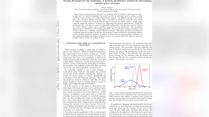
When facing a heavily-favored opponent, an underdog must be willing to assume greater-than-average risk. In statistical language, one would say that an underdog must be willing to adopt a strategy whose outcome has a larger-than-average variance. The difficult question is how much risk a team should be willing to accept. This is equivalent to asking how much the team should be willing to sacrifice from its mean score in order to increase the score’s variance. In this paper a general, analytical method is developed for addressing this question quantitatively. Under the assumption that every play in a game is statistically independent, both the mean and the variance of a team’s offensive output can be described using the binomial distribution. This description allows for direct calculations of the winning probability when a particular strategy is employed, and therefore allows one to calculate optimal offensive strategies. This paper develops this method for calculating optimal strategies exactly and then presents a simple heuristic for determining whether a given strategy should be adopted. A number of interesting and counterintuitive examples are then explored, including the merits of stalling for time, the run/pass/Hail Mary choice in American football, and the correct use of Hack-a-Shaq.

💡 Research Summary

The paper presents a quantitative framework for underdog teams to increase their probability of winning by deliberately increasing the variance of their scoring outcomes, even at the cost of a lower expected score. The authors model every offensive play as an independent Bernoulli trial characterized by a success probability p and a point value v. For a set of play types i, each executed N_i times, the team’s expected total points μ and variance σ² are given by μ = Σ v_i N_i p_i and σ² = Σ v_i² N_i p_i(1 − p_i). This formulation allows the total score distribution to be expressed as a product of binomial distributions, which is exact under the independence assumption.

Winning probability is defined as the overlap between the probability density functions of the underdog’s final score and that of the opponent. While an exact calculation can be performed by enumerating all possible outcomes (as detailed in the Appendix), the authors show that for a realistic number of remaining plays (N > 5), the Central Limit Theorem (CLT) provides an accurate approximation. The score differential Δ = (team score) − (opponent score) becomes Gaussian with mean μ − μ_opp and variance σ² + σ²_opp. The probability of victory is then P ≈ ½