lgcp An R Package for Inference with Spatio-Temporal Log-Gaussian Cox Processes

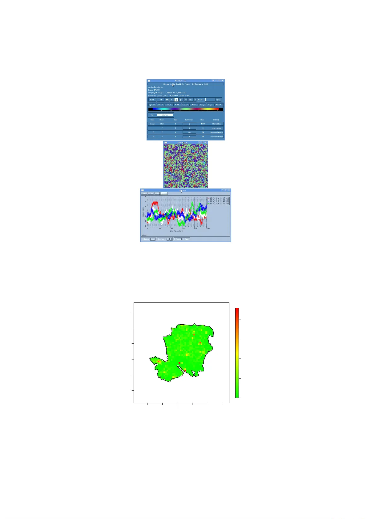
lgcp – An R P ac k age for Inference with Spatio-T emp oral Log-Gaussian Co x Pro cesses Benjamin M. T a ylor Lancaster Univ ersity , UK Tilman M. Da vies Massey Univ ersity , NZ Barry S. Ro wlingson Lancaster Univ ersity , UK P eter J. Diggle Lancaster Univ ersity , UK Abstract This pap er introduces an R pack age for spatio-temp oral prediction and forecasting for log-Gaussian Co x pro cesses. The main computational to ol for these mo dels is Marko v c hain Mon te Carlo and the new pac k age, lgcp , therefore also pro vides an extensible suite of functions for implemen ting MCMC algorithms for processes of this t yp e. The modelling framew ork and details of inferential pro cedures are first pres ented b efore a tour of lgcp functionalit y is giv en via a w alk-through data-analysis. T opics co vere d include reading in and con verting data, estimation of the k ey comp onents and parameters of the mo del, sp ecifying output and simulation quantities, computation of Monte Carlo exp ectations, p ost-processing and simulation of data sets. Keywor ds : Co x pro cess; R ; spatio-temp oral p oin t pro cess. 1. In tro duction This article in tro duces a new R pack age, lgcp , for inference with spatio-temporal log-Gaussian Co x pro cesses R Developmen t Core T eam ( 2011 ). The w ork was motiv ated by applications in disease surveillance, where the ma jor fo cus of scientific in terest is on whether, and if so where and when, cases form unexplained clusters within a spatial region W and time-interv al (0 , T ) of interest. It will b e assumed that b oth the lo cation and time of each case is known, at least to a sufficiently fine resolution that a p oint pro cess mo delling framew ork is natural. In general, the aims of statistical analysis include mo del formulation, parameter estimation and spatio-temp oral prediction. The lgcp pack age includes some functionality for parameter estimation and diagnostic chec king, mostly b y link ages with other R pac k ages for spatial statistics. Ho w ever, and consisten t with the scientific fo cus b eing on disease surveillance, the curren t version of the pack age places particular emphasis on real-time predictive inference. Sp ecifically , using the mo delling framework of a Co x pro cess with sto ch astic in tensity R ( x, t ) = exp {Y ( x, t ) } , where Y ( x, t ) is a Gaussian pro cess, the pac k age enables the user to draw samples from the join t predictive distribution of R ( x, t + k ) given data up to and including time t ≤ T , for any set of lo cations x ∈ W and forecast lead time k ≥ 0. In the surv eillance setting, these samples w ould typically b e used to ev aluate the predictive probabilit y that the intensit y at a particular lo cation and time exceeds a sp ecified interv en tion threshold; see, for example, 2 lgcp – An R Pac k age for Inference with Spatio-T emp oral Log-Gaussian Co x Pro cesses Diggle, Ro wlingson, and Su ( 2005 ). The lgcp pack age makes extensiv e use of spatstat functions and data structures ( Badde- ley and T urner 2005 ). Other imp ortant dep endencies are: the sp pack age, which also sup- plies some data structures and functions ( Pebesma and Biv and 2005 ; Biv and, Pebesma, and Gomez-Rubio 2008 ); the suite of cov ariance functions provided b y the RandomFields pack age ( Sc hlather 2001 ); the rpanel pack age to facilitat e minimum-con trast parameter estimati on routines ( Bowman, Cra wford, Alexander, and Bo wman 2007 ; Bowman, Gibson, Scott, and Cra wford 2010 ); and the ncdf pac k age for rapid access to massive datasets for p ost-pro cessing ( Pierce 2011 ). In Section 2 the log-Gaussian Cox pro cess is in tro duced. Section 3 gives a review on methods of inference for log-Gaussian Cox pro cesses. Section 4 is an ov erview of the pack age by wa y of a walk-through example, cov ering: reading in data (Section 4.1 ); estimating comp onents of the model and asso ciated parameters (Sections 4.2 and 4.3 ); setting up and running the model (Sections 4.4 and 4.5 ); and p ost-pro cessing of command outputs (Section 4.6 ). Some p ossible extensions of the pack age are given in Section 5 . The app endices give further informat ion on the rotation of observ ation windows (Appendix A ), sim ulation of data (App endix B ) and information ab out the spatialAtRisk class of ob jects (App endix C ), whic h may b e useful for reference purp oses. 2. Spatio-T emporal log-Gaussian Co x pro cesses Let W ⊂ R 2 b e an observ ation windo w in space and T ⊂ R ≥ 0 b e an in terv al of time of in terest. Cases o ccur at spatio-temp oral p ositions ( x, t ) ∈ W × T according to an inhomogeneous spatio- temp oral Cox pro cess, i.e., a P oisson pro cess with a sto chastic intensit y R ( x, t ). The num b er of cases, X S, [ t 1 ,t 2 ] , arising in any S ⊆ W during the in terv al [ t 1 , t 2 ] ⊆ T is then Poi sson distributed conditional on R , X S, [ t 1 ,t 2 ] ∼ P oisson  Z S Z t 2 t 1 R ( s, t )d s d t  . (1) F ollowing Diggle et al. ( 2005 ), the intensit y is decomp osed multiplicativ ely as, R ( s, t ) = λ ( s ) µ ( t ) exp {Y ( s, t ) } . (2) In Equation 2 ,the fixe d sp atial c omp onent , λ : R 2 7→ R ≥ 0 , is a known function, prop ortional to the p opulation at risk at each p oin t in space and scaled so that, Z W λ ( s )d s = 1 , (3) whilst the fixe d temp or al c omp onent , µ : R ≥ 0 7→ R ≥ 0 , is also a known function such that, µ ( t ) = lim δ t → 0  E [ X W,δt ] | δ t |  . (4) The function Y is a Gaussian process, con tinuous in both space and time. In the nomenclature of epidemiology , the comp onents λ and µ determine the endemic spatial and temp oral com- p onen t of the p opulation at risk; whereas Y captu res the residual v ariation, or the epidemic comp onen t. Benjamin M. T aylor, Tilman M. Da vies, Barry S. Rowlingson, P eter J. Diggle 3 The Gaussian pro cess, Y , is second order stationary with minimally-parametrised co v ariance function, co v [ Y ( s 1 , t 1 ) , Y ( s 2 , t 2 )] = σ 2 r ( || s 2 − s 1 || ; φ ) exp {− θ ( t 2 − t 1 ) } , (5) where || · || is a suitable norm on R 2 , for instance the Euclidean norm, and σ, φ, θ > 0 are kno wn parameters. In the lgcp pack age, the isotropic spatial correlation function, r , may tak e one of sev eral forms and possibly require additional parameters (in lgcp , this can b e selected from any of the compatible models in the function CovarianceFct from the RandomFields pac k age). The parameter σ scales the log-in tensity , whilst the parameters φ and θ gov ern the rates at whic h the correlation function decreases in space and in time, resp ectively . The mean of the pr o cess Y is set equal to − σ 2 / 2 so as to give E [exp {Y } ] = 1, hence the endemic/epidemic analogy ab o ve. 3. Inference As in Møller, Syv ersv een, and W aagep etersen ( 1998 ), Brix and Diggle ( 2001 ) and Diggle et al. ( 2005 ), a discretised version of the ab ov e mo del will b e considered, defined on a regular grid o ver space and time. Observ ations, X , are then treated as cell counts on this grid. The discrete versi on of Y will b e denoted Y ; since Y is a finite collection of random v ariables, the prop erties of Y imply that Y has a multiv ariate Gaussian density with approximate co v ariance matrix Σ, whose elements are calculated b y ev aluating Equation 5 at the centroids of t he spatio-temporal grid cells. Without loss of generalit y , unit time-incremen ts are assumed and ev ents can b e though t of as occurring “at” in teger times t . Let X t denote an observ ation o ver the spatial grid at time t , and X t 1 : t 2 denote the observ ations at times t 1 , t 1 + 1 , . . . , t 2 . F or predictive inference about Y , samples from the conditional distribution of the laten t field, Y t , giv en the observ ations to date, X 1: t w ould b e drawn, but this is infeasible b ecause the dimensionalit y of the required in tegration increases without limit as time progresses. An alternativ e, as suggested by Brix and Diggle ( 2001 ), is to sample from Y t 1 : t 2 giv en X t 1 : t 2 , π ( Y t 1 : t 2 | X t 1 : t 2 ) ∝ π ( X t 1 : t 2 | Y t 1 : t 2 ) π ( Y t 1 : t 2 ) , (6) where t 1 = t 2 − p for some small positive integer p . The justification for this approac h is that observ ations from the remote past ha ve a negligible effect on inference for the curren t state, Y t . In order to ev aluate π ( Y t 1 : t 2 ) in Equation 6 , the parameters of the pro cess Y m ust either b e kno wn or estimated from the data. Estimation of σ , φ and θ may be achiev ed either in a Ba ye sian framework, or b y one of a n umber of more ad ho c metho ds. The methods implemen ted in the current version of the lgcp pack age fall in to the latter category and are describ ed in Brix and Diggle ( 2001 ) and Diggle et al. ( 2005 ). Briefl y , this inv olv es matching empirical and theoretical estimates of the second-moment prop erties of the mo del. F or the spatial cov ariance parameters σ and φ , the inhomogeneous K -function, or g function are used ( Baddeley , Møller, and W aagepetersen 2000 ). The auto correlation function of the total ev ent-coun ts per unit time-interv al is used for estimating the temp oral correlation parameter θ . The estimated parameter v alues can then b e used to implemen t plug-in-prediction for the laten t field Y t . 3.1. Discretising and the fas t-F ourier trans form 4 lgcp – An R Pac k age for Inference with Spatio-T emp oral Log-Gaussian Co x Pro cesses The first barrier to inference is computation of the cov ariance matrix, Σ, which ev en for relativ ely coarse grids is v ery large. F ortunately , for regular spatial grids of size 2 m × 2 n , there exist fast methods for computing this based on the discrete F ourier transform ( W o o d and Chan 1994 ). The general idea is to embed Σ in a symmetric circulant matrix, C = Q Λ Q ∗ , where Λ is a diagonal matrix of eigenv alues of C , Q is a unitary matrix and ∗ denotes the Hermitian transp ose. The en tries of Q are giv en b y the discrete F ourier transform. Computation of C 1 / 2 , whic h is useful for b oth simulation and ev aluation of the density of Y , is then straightforw ard using the fact that C 1 / 2 = Q Λ 1 / 2 Q ∗ . 3.2. The Metrop olis-adjusted Langevin algorithm Mon te Carlo sim ulation from π ( Y t 1 : t 2 | X t 1 : t 2 ) is made more efficien t by w orking with a linear transformation of Y , partially determined by the matrix C as described below. The lgcp pac k age returns results p ertaining to Y on a grid of size M × N ≡ 2 m × 2 n for p ositive in tegers m and n specified by the user, which is ext ended to a grid of size 2 M × 2 N for computation ( Møller et al. 1998 ). W riting Γ t = Λ − 1 / 2 Q ( Y t − µ ), the target of interest is given b y , π (Γ t 1 : t 2 | X t 1 : t 2 ) ∝ " t 2 Y t = t 1 π ( X t | Y t ) # " π (Γ t 1 ) t 2 Y t = t 1 +1 π (Γ t | Γ t − 1 ) # , (7) where the first term on the right hand side of Equation 7 corresp onds to the first brack eted term on the right hand side of Equation 6 and the second brack eted term is the join t densit y , log { π (Γ t 1 : t 2 ) } . Because Γ is an Ornstein-Uhlenbec k pro cess in time, the transition density , π (Γ t | Γ t − 1 ), has an explicit expression as a Gaussian densit y; see Brix and Diggle ( 2001 ). Since the gradien t of the transition density can also be written down explicitly , a natural and efficien t MCMC metho d for sampling from the predictiv e density of in terest (Equation 7 ), is a Metrop olis-Hastings algorithm with a Langevin-type prop osal ( Rob erts and Tweedie 1996 ), q (Γ , Γ 0 ) = N  Γ 0 ; Γ + 1 2 ∇ log { π (Γ | X ) } , h 2 I  , where N( y ; m, v ) denotes a Gaussian densit y with mean m and v ariance v ev aluated at y , I is the iden tity matrix and h > 0 is a scaling parameter ( Metrop olis, Rosen bluth, Rosen bluth, T eller, and T eller 1953 ; Hastings 1970 ). V arious theoretical results exist concerning the optimal acceptance probability of the MALA (Metrop olis-Adjusted Langevin Algorithm) – see Rob erts and Rosen thal ( 1998 ) and Rob erts and Rosen thal ( 2001 ) for example. In practical applications, the target acceptance probabilit y is often set to 0.574, which would b e appro ximately optimal for a Gaussian target as the dimension of the problem tends to infinit y . An algorithm for the automatic c hoice of h , so that this acceptance probabilit y is ac hieved without disturbing the ergo dic prop ert y of the c hain, is also straightforw ard to implement, see Andrieu and Thoms ( 2008 ). 4. In tro ducing the lgcp pac k age 4.1. Reading-in and conv erting data Benjamin M. T aylor, Tilman M. Da vies, Barry S. Rowlingson, P eter J. Diggle 5 The generic data-format of in terest is ( x i , y i , t i ) : i = 1 , ..., n , where the ( x i , y i ) are the lo cations and t i the times of occurrence of even ts in W × ( A, B ), where W is a p olygonal observ ation window and ( A, B ) the time-interv al within which even ts are observed. In the follo wing example x , y and t are R ob jects giving the lo cation and time of even ts and win is a spatstat ob ject of class owin sp ecifying the p olygonal observ ation window ( Baddeley and T urner 2005 ). An example of constructing an appropriate owin ob ject from ESRI shap efiles is giv en in the pack age vignette (type vignette("lgcp") ). R> data <- cbind(x,y,t) R> tlim <- c(0,100) R> win window: polygonal boundary enclosing rectangle: [381.7342, 509.7 342] x [64.14505, 192.14505 ] units The first task for the user is to conv ert this in to a space-time planar p oin t pattern ob ject ie. one of class stppp , pro vided by lgcp . An ob ject of class stppp is easily created: R> xyt <- stppp(list(data=data,tlim=t lim,window=win)) R> xyt Space-time point pattern planar point pattern: 10069 points window: polygonal boundary enclosing rectangle: [381.7342, 509.7 342] x [64.14505, 192.14505 ] units Time Window : [ 0 , 100 ] 4.2. Estimating the spatial and temporal comp onent There are many wa ys to estimate the fixed spatial and temp oral comp onent s of the log- Gaussian Cox process. The fixed spatial comp onen t, λ ( s ), represen ts the spatial in tensity of ev ents, av eraged ov er time and scaled to in tegrate to 1 ov er the observ ation windo w W . In epidemiological settings, this t ypically corresponds to the spatial distribution of the p opu- lation at risk, although this information ma y not b e directly av ailable. The fixed temp oral comp onen t, µ ( t ), is the mean num b er of ev ents in W p er unit time. Where the relev ant demographic information is unav ailable to sp ecify λ ( s ) and µ ( t ) directly , lgcp provi des basic functionalit y to estimate them from the data. The function lambdaEst is an interactiv e implemen tation of a ker nel metho d for estimating λ ( s ) as in the following example: R> den <- lambdaEst(xyt,axes=TRUE) R> plot(den) This calls an rpanel to ol ( Bo wman et al. 2007 ) for estimating λ (see Figure 1 ); once the user is happ y with the result, clic king on “OK” closes the panel and the kernel density estimate is stored in the R ob ject den of class im (a spatstat pixel image ob ject). The estimate of λ 6 lgcp – An R Pac k age for Inference with Spatio-T emp oral Log-Gaussian Co x Pro cesses Figure 1: Cho osing a kernel densit y estimate of λ ( s ). can then b e plotted in the usual w ay . The parameters bandwidth and adjust in this GUI relate to the arguments from the spatstat function density.ppp ; the former corresp onds to the argumen t sigma and the latter to the argument of the same name. The lgcp pac k age provides metho ds for co ercing pixel-images like den to ob jects of class spatialAtRisk , whic h can th en b e used in parameter estimation and in the MALA algorithm to b e discussed later; further useful information on the spatialAtRisk class is pro vided in App endix C . R> sar <- spatialAtRisk(den) SpatialAtRisk object X range : [382.3742066569,509.0942066 56898] Y range : [64.785045372051,191.505045 372051] dim : 100 x 100 F or the temp oral comp onent, µ ( t ), the user m ust pro vide an ob ject that can b e co erced into one of class temporalAtRisk . Ob jects of class temporalAtRisk are non-negativ e functions of tim e ov er an observ ation time- windo w of in terest, whic h m ust be the same as the time-windo w of the stppp data ob ject, xyt . In some applications ( Diggle et al. 2005 ), µ ( t ) migh t represen t the fitted v alues of a parametric mo del for the case coun ts o ver time. As it is not p ossible to pro vide generic functionalit y for parametric µ ( t ), a simple non-parametric estimate of µ can b e generated using the function muEst : R> mut1 <- muEst(xyt) R> mut1 temporalAtRisk object Time Window : [ 0 , 100 ] Benjamin M. T aylor, Tilman M. Da vies, Barry S. Rowlingson, P eter J. Diggle 7 In order to retain p ositivit y , muEst fits a lo cally-weigh ted p olynomial regression estimate (the R function lowess ) to the square ro ot of the in terv al counts and returns the square of this smo othed estimate (see Figure 2 ). The amoun t of smoothing is controlled by the lowess argumen t f which sp ecifies the prop ortion of p oints in the plot whic h influence the smo othed estimate at each v alue (see ?lowess ), for example muEst(xyt,f=0.1) . If the user wishes to sp ecify a constan t time-trend, µ ( t ) = µ , the command R> mut <- constantInTime(xyt) returns the appropriate temporalAtRisk ob ject, correctly scaled as in Equat ion 4 . The 0 20 40 60 80 100 80 85 90 95 100 105 110 time at_risk Figure 2: Estimating µ ( t ): the output from plot(mut1) . fixed temp oral comp onent can b e also b e supp lied either as a vector or as a function that is automatically co erced to a temporalAtRisk ob ject and scaled to achiev e the condition in Equation 4 . 4.3. Estimating parameters After estimating λ ( s ) and µ ( t ), the next step in the analysis is to estimate the cov ariance parameters of the pro cess Y . lgcp pro vides basic moment-based metho ds for this in the form of rpanel GUIs that allo w the user to c ho ose σ , φ and θ by eye ( Bowman et al. 2007 ). P arameter estimation by ey e is b oth fast and reasonably robust and moreov er emphasizes the fact that the underlying metho ds are ad ho c . As men tioned ab ov e, it is p ossible to implement principled Ba yesian parameter estimation for this mo del by integrating ov er the discretised laten t-field, Y ; this is a planned extension to the pac k age (see Section 5 ). The spatial correlation parameters σ and φ can b e estimated either from the pair correlation function, g , or th e inhomogeneous K function ( Baddeley et al. 2000 ). F ollowing Brix and Diggle ( 2001 ) and Diggle et al. ( 2005 ), the corresp onding functions in lgcp estimate v ersions of these tw o functions b y av eraging temp orally lo calised v ersions. The resp ective commands for doing so are: R> gin <- ginhomAverage(xyt,spatial.i ntensity=sar,temporal.intensity=mut) R> kin <- KinhomAverage(xyt,spatial.i ntensity=sar,temporal.intensity=mut) 8 lgcp – An R Pac k age for Inference with Spatio-T emp oral Log-Gaussian Co x Pro cesses The parameters are then estimated using either of the follo wing: R> sigmaphi1 <- spatialparsEst(gin,si gma.range=c(0,10),phi.range=c(0,10)) R> sigmaphi2 <- spatialparsEst(kin,si gma.range=c(0,10),phi.range=c(0,10)) These in vok e another call to rpanel , which pro duces the plots in Figure 3 . The user’s task is to matc h the orange theoretical function with the blac k empirical coun terpart. The user Figure 3: Estimating σ and φ : left via the pair correlation function and right via the inhomogeneous K function. can choose b et ween the exp onential, Mat ´ ern or Whittle families of correlation functions; see ?CovarianceFct from the RandomFields pac k age. F or the Mat ´ ern or Whittle families an additional shap e parameter, ν , is sp ecified by the user and treated as a known constan t. This is because ν is kno wn to be difficult to estimate. A recommended strategy is to c ho ose betw een a discrete set of candidate v alues; for example, in the Mat´ ern family the integer part of ν giv es the num b er of times the underlying Gaussian pro cess is mean-square differentiable. The resulting estimated parameters are returned in list ob jects (e.g., sigmaphi1 or sigmaphi2 ) with sigmaphi1$sigma and sigmaphi1$phi returning the required v alues of σ and φ . In the co de b elo w, note that these v alues hav e b een input man ually as respectively 1 . 6 and 1 . 9. The user has additional control ov er the minimum con trast estimation, for example the range of ev aluation, though sensible defaults are provided automatically by the embedded spatstat functions. The temp oral correlation parameter, θ , can be estimated using the function thetaEst ; this requires σ , φ and µ ( t ) to hav e b een estimated b eforehand. F or example, the call R> theta <- thetaEst(xyt,spatial.inte nsity=sar, temporal.intensity=mut, sigma=1.6,phi=1.9) giv es the result sho wn in Figure 4 . Note that again, in the co de below the estimated v alue of 1 . 4 has b een input manually . 4.4. The command lgcpPredict Benjamin M. T aylor, Tilman M. Da vies, Barry S. Rowlingson, P eter J. Diggle 9 Figure 4: Estimating θ . The main function in the lgcp pack age is lgcpPredict . This uses an MCMC method to pro duce samples and summary statistics from the predictiv e dist ribution of the discre tised pro cess Y , treating previously obtained estimates of λ ( s ), µ ( t ), and the co v ariance parameters as known quan tities. The MCMC algorithm is inv ok ed by the command lgcpPredict , whose argumen ts are as follows: R> args(lgcpPredict) function (xyt, T, laglength, model.paramet ers = lgcppars(), spatial.covmodel = "exponential", cov pars = c(), cellwidth = NULL, gridsize = NULL, spatial.intensity, tempor al.intensity, mcmc.control, output.control = setoutput(), autorot ate = FALSE, gradtrunc = NULL) Data and mo del sp e cific ation The argumen t xyt is the stppp ob ject that contains the data, T is the time-p oin t of interest for prediction (c.f., the time t 2 in Section 3 ) and laglength tells the algorithm the n umber of previous time-p oin ts whose data should b e included. Mo del parameters are set using the model.parameters argumen t; for example, R> lgcppars(sigma=1.6,phi=1. 9,theta=1.4) has the obvious in terpretation. The spatial cov ariance mo del and an y additional parameters are sp ecified using the spatial.covmodel and covpars argumen ts; these may come from an y of the compatible co v ariance functions detailed in ?CovarianceFct from the RandomFields pac k age. The physical dimensions of the grid cells can b e set using either the cellwidth or gridsize argumen ts, the second of which giv es the n umber of cells in the x and y directions (these n umbers are automatically extended to b e a p o wer of tw o for the fast-F ourier trans- form). The spatial.intensity and temporal.intensit y arguments sp ecify the previously obtained estimates of λ ( s ) and µ ( t ), resp ectivel y . 10 lgcp – An R Pac k age for Inference with Spatio-T emp oral Log-Gaussian Co x Pro cesses It remains to set the MCMC parameters and output contr ols; these will no w b e discussed. Contr ol ling MALA and p erforming adaptive MCMC The mcmc.control argumen t of lgcpPredict sp ecifies the MCMC implementation and is set using the mcmcpars function: R> args(mcmcpars) function (mala.length, burnin, retain , inits = NULL, MCMCdiag = 0, adaptivescheme) Here, mal a.length is the num b er of iterations to p erform, burnin is the num b er of itera- tions to throw aw ay at the start and retain is the frequency at which to store or p erform computations; for example, retain=1 0 performs an action every 10th iteration. The optional argumen t inits can b e used to set initial v alues of Γ for the algorithm, and is in tended for adv anced use. The initial v alues are stored in a list ob ject of length laglength +1, each ele- men t b eing a matrix of dimension 2 M × 2 N . The option MCMCdiag allows the user to sav e a sample of the Γ chains; if MCMCdiag=5 for example, then a random sample of 5 MCMC chains from 5 different cells are stored; these can be used to assess the con vergence or mixing of the c hain in the p ost-pro cessing stage. The MALA prop osal tuning parameter h in Section 3.2 must also b e c hosen. The most straigh tforward w a y to do this is to set adaptivescheme=consta nth(0.001) , which giv es h = 0 . 001. Without a length y tuning pro cess, the v alue of h that optimizes the mixing of the algorithm is not known. One solution to the problem of ha ving to choose a scaling parameter from pilot runs is to use adaptiv e MCMC ( Rob erts and Rosenthal 2009 ; Andrieu and Thoms 2008 ). Adaptiv e MCMC algorithms use information from the realisation of an MCMC c hain to make adjustments to the proposal k ernel. The Marko v property is therefore no longer satisfied and some care m ust b e tak en to ensure that the corre ct ergo dic distribution is preserved. An elegan t metho d, introduced b y Andrieu and Thoms ( 2008 ) uses a Robbins- Munro stochastic appro ximation up date to adapt the tuning parameter of the prop osal k ernel ( Robbins and Munro 1951 ). The idea is to up date the tuning parameter at each iteration of the sampler according to the iterativ e scheme, h ( i +1) = h ( i ) + η ( i +1) ( α ( i ) − α opt ) , (8) where h ( i ) and α ( i ) are the tun ing parameter and acceptance probabilit y at iteration i and α opt is the target acceptance probability . F or Gaussian targets, and in the limit as the dimension of the problem tends to infinity , an appropriate target acceptance probability for MALA algorithms is α opt = 0 . 574 ( Roberts and Rosenthal 2001 ). The sequence { η ( i ) } is chosen so that P ∞ i =0 η ( i ) is infinite but for an y  > 0, P ∞ i =0  η ( i )  1+  is finite. These tw o conditions ensure that an y v alue of h can b e reached, but in a wa y that main tains the ergodic b ehaviour of the c hain. One class of sequences with this prop erty is, η ( i ) = C i α , (9) where α ∈ (0 , 1] and C > 0 ( Andrieu and Thoms 2008 ). The tuning constan ts for this algorithm are set with the function andrieuthomsh . Benjamin M. T aylor, Tilman M. Da vies, Barry S. Rowlingson, P eter J. Diggle 11 R> args(andrieuthomsh) function (inith, alpha, C, targetacceptanc e = 0.574) In the abov e, inith is the initial v alue of h and the remaining argumen ts correspond to their coun terparts in the text ab ov e. The adv anced user can also write their o wn adaptiv e scheme, detailed examples of whic h are pro vided in the pac k age vignette. Briefly , writing an adaptiv e MCMC sc heme in v olves writ ing t wo functions to tell R how to initialise and up date the v alues of h . This ma y sound simple, but it is crucial that these functions preserv e the correct ergo dic distribution of the MCMC c hain, an appreciation of these subtleties is essential b efore any attempt is made to co de suc h schemes. Sp e cifying output By default, lgcpPredict computes the mean and v ariance of Y and the mean and v ariance of exp { Y } (the relativ e risk) for each of the grid cells and time interv als of in terest. Additional storage and online computations are sp ecified by the output.control argument and the setoutput function: R> args(setoutput) function (gridfunction = NULL, gridmeans = NULL) The option gri dfunction is used to declare general operations p erform during simulation (for example, dumping the simulated Y s to disk), whilst user-defined Monte Carlo av erages are computed using gridmeans . A complete run of the MALA chain can b e sav ed using the dump2dir function: R> args(dump2dir) function (dirname, lastonly = TRUE, forceSave = FALSE) The user supplies a c haracter string, dirname , giving the name of a directory in whic h the results are to b e sav ed. The other arguments to dump2dir are, respectively , an option to sav e only the last grid (i.e., the time T grid) and to b ypass a safety message that w ould otherwise b e disp lay ed when dump2dir is in vok ed. The safet y message war ns the user of disk space requiremen ts for saving. F or example, on a 128 × 128 output grid using 5 da ys of data, 1000 sim ulations from the MALA will take up appro ximately 625 megabytes. Another option is to compute Mon te Carlo exp ectations, E π ( Y t 1 : t 2 | X t 1 : t 2 ) [ g ( Y t 1 : t 2 )] = Z W g ( Y t 1 : t 2 ) π ( Y t 1 : t 2 | X t 1 : t 2 )d Y t 1 : t 2 , (10) ≈ 1 n n X i =1 g ( Y ( i ) t 1 : t 2 ) (11) where g is a function of interest, Y ( i ) t 1 : t 2 is the i th retained sample from the target and n is the total num b er of retained iterations. F or example, to compute the mean of Y t 1 : t 2 , set 12 lgcp – An R Pac k age for Inference with Spatio-T emp oral Log-Gaussian Co x Pro cesses g ( Y t 1 : t 2 ) = Y t 1 : t 2 . The output from suc h a Monte Carlo a verage would then b e a set of t 2 − t 1 grids, eac h cell of whic h is equal to the mean o ver all retained iterations of the algorithm. In the context of setting up the gridmeans option to compute the Mon te Carlo mean, the user w ould define a function g as R> gfun <- function(Y){ return(Y) } and input this to the MALA run using the function MonteCarloAverage , R> args(MonteCarloAverage) function (funlist, lastonly = TRUE) Here, funlist is either a list or a character vector giving the names of the function(s) g . The sp ecific syntax for the example ab ov e would be a call of the form MonteCarloAverage("gfu n") . The functions of in terest (e.g., gfun abov e) are assumed to act on eac h of the individual grids, Y t i , and return a grid of the same dimension. A second example arises in epidemiological studies where of clinical interest to kno w whether, at any lo cation s , the ratio of current to exp ected risk exceeded a pre-specified in terven tion threshold; see, for example, Diggle et al. ( 2005 ), where real-time predictions of relative risk are presented as maps of exceedance probabilities, P { exp( Y t ) > k | X 1: t } for a pre-sp ecified threshold k . An y such exceedance probabilit y can b e expressed as an exp ectation, P [exp( Y t 1 : t 2 ) > k ] = E π ( Y t 1 : t 2 | X t 1 : t 2 ) [ I ( Y t 1 : t 2 > k )] = 1 n n X i =1 I ( Y ( i ) t 1 : t 2 > k ) , where I is the indicator function, and a Mon te Carlo appro ximation can therefore be computed on-line using MonteCarloAverage . The corresp onding function g is g ( Y t 1 : t 2 ) = I ( Y t 1 : t 2 > k ) . Exceedance probabilities are made av ailable directly within lgcp b y the function exceedProbs . T o make use of this facility , the user sp ecifies the thresholds of in terest, for example 1.5, 2 and 3, then creates a function to compute the required exceedances: R> exceed <- exceedProbs(c(1.5,2,3)) The ob ject exceed is no w a function that returns the exceedance probabilities as an array ob- ject of dimension M × N × 3. This function can b e passed through to the gridmeans option, to- gether with the previously defined gfun , via gridmeans=MonteC arloAverage(c("gfun","exceed") . The lgcpPredict function then returns p oint-wise predictive means and three sets of ex- ceedance probabilities. Note that, the example function gfun is included for illustrativ e purp oses only and is in fact redundant, as lgcpPredict automatically returns the predictive mean (and v ariance) of Y . Benjamin M. T aylor, Tilman M. Da vies, Barry S. Rowlingson, P eter J. Diggle 13 R otation T esting whether estimation can pro ceed more efficien tly in a rotated space is described in detail in App endix A . Note that if the data and observ ation window are rotated, then λ must also b e rotated to retain compatibility . If λ was estimated in the original frame of reference and autorotate=TRUE , then lgcpPredi ct will automatically rotate λ if it is computationally w orthwhile to do so. F or λ sp ecified as a grid, either directly or via an ob ject of class im , then a small amount of information loss o ccurs in the rotation because the square cells in the original orien tation b ecome misaligned with the axes in the rotated space and vice-v ersa. If λ is sp ecified by a con tinuous function, then no suc h loss o ccurs. Gr adient trunc ation One undesirable prop ert y of the Metrop olis-adjusted Langevin algorithm is that the chain is prone to taking very long excursions from the mo de of the target; this b ehaviour can hav e a detrimen tal effect on the mixing of the c hain and consequen tly on any results. The tendency to make long excursions is caused by instability in the computation of the gradient vector, but the issue is relatively straigh tforward to rectify without affecting conv ergence prop erties ( Møller et al. 1998 ). The key is to truncate the gradient v ector if it b ecomes to o large. If gradtrunc=NULL , then an appropriate truncation is automatically selected by the co de. As far as the authors are aw are, there are no published guidelines for selecting this truncation parameter. The curren t version of the lgcp pack age uses the maxim um achiev ed gradient o ver a set of 100 indep enden t realisations of Γ t 1 : t 2 . 4.5. Running When all of the ab o ve options ha ve b een specified, the MALA algorithm can be called as follo ws: R> lg <- lgcpPredict(xyt=xyt, T=50, laglength=5, model.parameters=lgcppa rs(sigma=1.6,phi=1.9,theta=1.4), cellwidth=2, spatial.intensity=sar, temporal.intensity=mut, mcmc.control=mcmcpars(m ala.length=120000,burnin=20000, retain=100,MCMCdiag=5, adaptivescheme=andrieut homsh(inith=1,alpha=0.5,C=1, targetacceptance=0.574) ), output.control=setoutpu t(gridfunction= dump2dir(dirname="C:/My Directory"), gridmeans=MonteCarloAve rage("exceed",lastonly=TRUE))) The abov e call assumes that the spatial co v ariance mo del is exponential, that no rotation i s to b e p erformed and that the user wishes to ha ve lgcpPredict compute an appropriate gradi- en t truncation automatically . The arguments spatial.inte nsity and temporal.intensity relate to the spatial and temp oral inten sities, estimated in Section 4.2 ; note that the chosen 14 lgcp – An R Pac k age for Inference with Spatio-T emp oral Log-Gaussian Co x Pro cesses temp oral mo del is constan t in time. The option lastonly=TRUE in MonteCarloAverage has the effect of only p erforming the computation on data from the last time p oin t, to sav e disk space. A similar option is a v ailable for the dump2dir function. The simulated example uses data from times 45 to 50 inclusiv e, 120,000 iterations, of whic h the first 20,000 are treated as burn-in, and retains every 100th sample. F or diagnostic chec king, a sample of MCMC Γ-chai ns is also sav ed for eac h of five randomly selected grid-cells. The observ ation windo w is appro ximately 100km square, so the sp ecified cell width of 2km giv es an output grid of size 64 × 64, i.e., computation is carried out on a 128 × 128 grid. The complete run is sa ved to disk and exceedance probabilities are computed for the last time-point only . During sim ulation, a progress bar is display ed giving the p ercentage of iterations completed. 4.6. P ost-pro cessing The stored output lg is an ob ject of class lgcpPredict . T yping lg in to the console prin ts out information ab out the run: R> lg lgcpPredict object. General Information ------------------- FFT Gridsize: [ 128 , 128 ] Data: Time | 45 46 47 48 49 50 Counts | 103 346 108 100 76 69 Parameters: sigma=1.6, phi=1.9, theta =1.4 Dump Directory: C:/MyDirectory Grid Averages: Function Output Class exceed array Time taken: 14.148 hours MCMC Information ---------------- Number Iterations: 120000 Burn-in: 20000 Thinning: 100 Mean Acceptance: 0.567 Adaptive Scheme: andrieuthomsh Last h: 0.001 Information returned includes the FFT grid size used in computation; the coun t data for each da y; the parameters used; the directory , if sp ecified, to which the simulation w as dump ed; a Benjamin M. T aylor, Tilman M. Da vies, Barry S. Rowlingson, P eter J. Diggle 15 list of MonteCarloAverage functions together with the R class of their returned v alues; the time tak en to do the sim ulation; and information on the MCMC run. Extr acting information The cell-wise mean and v ariance of Y computed via Mon te Carlo can alwa ys be extracted using meanfield(lg) and varfield(lg) , resp ectively . The calls rr(lg) , serr(lg) and intens(lg) return resp ectively the Monte Carlo mean relative risk (the mean of exp { Y } ), the standard error of the relative risk and the estimated cell-wise mean Poisson intensit y . The x and y co ordinates for the grid output are obtained via xvals(lg) and yvals(lg) . If in vok ed, the commands gridfun(lg) and gridav(lg) return respectively the gridfunction and gridmeans options of the setoutput argumen t of the lgcpPredict function, whilst window(lg) returns the observ ation windo w. Note that the structure pro duced by gav <- gridav(lg) is a list of length 2. The first el- emen t of gav , retriev ed with gav$names , is a list of the function names given in the call to Mo nteCarloAverage . The second elemen t, gav$output , is a list of the function out- puts; the i th elemen t in the list b eing the output from the funct ion corresp onding to th e i th element of gav$names . T o return the output for a sp ecific function, use the syn tax gridav(lg,fun="exceed") , which in this case returns the exceedance probabilities, for ex- ample. Plotting Plots of the Monte Carlo mean relative risk and standard errors can b e obtained with the commands: R> plot(lg,xlab="x coordinate",yl ab="y coordinate") R> plot(lg,type="serr",xlab= "x coordinate",yla b="y coordinate") These commands pro duce a series of plots corresp onding to each time step under considera- tion; the plots sho wn in Figure 5 are from the last time step, time 50. T o plot the mean Poisson in tensity instead of the relativ e risk, the optional argument type can b e set in the ab ov e: R> plot(lg,type="intensity", xlab="x coordinate",ylab="y coordinate") The cases for eac h time step are also plotted b y default. MCMC diagnostics MCMC diagnostics for the chain can either b e based on a small sample of cells, sp ecified by the MCMCdiag argument of t he mcmcpars function, or via the full output fr om data dump ed to disk (see Section 4.6.4 ). The hvals command returns the v alue of h used at eac h iteration in the algorithm, the left hand plot in Figure 6 shows the v alues of h for the non-burn-in perio d of the chain; the adaptiv e algorithm was in tialised with h = 1, which v ery quickly con verged to around h = 0 . 0006. R> plot(hvals(lg)[20000:1200 00],type="l",xlab="Iteration",ylab="h") R> tr <- mcmctrace(lg) R> plot(tr,idx=1:5) 16 lgcp – An R Pac k age for Inference with Spatio-T emp oral Log-Gaussian Co x Pro cesses 400 420 440 460 480 500 80 100 120 140 160 180 Relative Risk x coordinate y coordinate 2 4 6 8 10 + + + + + + + + + + + + + + + + + + + + + + + + + + + + + + + + + + + + + + + + + + + + + + + + + + + + + + + + + + + + + + + + + + + + + 400 420 440 460 480 500 80 100 120 140 160 180 S.E. Relative Risk x coordinate y coordinate 2 4 6 8 10 12 + + + + + + + + + + + + + + + + + + + + + + + + + + + + + + + + + + + + + + + + + + + + + + + + + + + + + + + + + + + + + + + + + + + + + Figure 5: Plots of the Monte Carlo mean relative risk (left) and asso ciated standard errors (righ t). T race plots, shown here in the right-han d panel of Figure 6 , are also av ailable using plot(tr) as in the abov e co de. Note that mcmctrace returns the trace for Γ. T o plot the autocorrelation function, the standard R function can b e used. F or example, acf(tr$trace[,1]) gives the acf of the first sav ed chain. 0e+00 2e+04 4e+04 6e+04 8e+04 1e+05 4e−04 5e−04 6e−04 7e−04 8e−04 Iteration h 0 200 400 600 800 1000 −2 −1 0 1 2 Iteration Y Cell Index 95,94 3,93 100,127 19,84 79,54 Figure 6: MCMC diagnostic plots. Left: plot of v alues of h tak en by the adaptive algorithm. Righ t: trace plots of the sav ed c hains from five grid cells. NetCDF The lgcp pack age provi des functions for accessing and p erforming computations on MCMC runs dump ed to disk. Because this can generate very large files, lgcp uses the cross-platform NetCDF file format for storage and rapid data access, as pro vided b y the pac k age ncdf ( Pierce 2011 ). Access to subsets of these stored data is via a file indexing system, which remov es the need to load the complete data int o memory . Subsets of data dump ed to disk can b e accessed with the extract function: Benjamin M. T aylor, Tilman M. Da vies, Barry S. Rowlingson, P eter J. Diggle 17 R> subsamp <- extract(lg,x=c(4,10),y= c(32,35),t=6,s=-1) whic h retur ns an array of dimension 7 × 4 × 1 × 1000 (recall there w ere 1000 retained it erations). The argumen ts x and y refer to the range of x and y indic es of the grid of in terest whilst t sp ecifies the time p oints of in terest. Note, how ever, that in this example times 45 through 50 w ere used for prediction, and t=6 here refers to the sixth of these time-p oin ts, i.e., time 50. Finally , s=-1 stipulates that all sim ulations are to b e returned . More generally , eac h argumen t of extract can b e sp ecified either as a range or set equal to − 1, in whic h case all of the data in that dimension are returned. The extract function can also extract MCMC traces from individual cells using, for example, extract(lg,x=37,y=12,t =6) . Should the user wish to extract data from a p olygonal subregion of the observ ation window, this can b e achiev ed with the command R> subsamp2 <- extract(lg,inWindow=wi n2,t=6) where win2 is a p olygonal observ ation window defined b elow. Here, win2 had b een selected using the follo wing commands: R> plot(window(lg)) R> win2 <- loc2poly() The first of the abov e commands plots the observ ation windo w, whilst the second is a wrapper function for the R function locator . When in v oked, loc2poly() allo ws the user to select areas of the observ ation windo w manually from the graphics device op ened by the first command: the user simply mak es a series of left clic ks, tra v ersing the required window in a single direction (i.e., clockwise or an ticlo ckwise), finishing the p olygon with a right click. The resulting selection is conv erted into a spatstat p olygonal owin ob ject. The user could also sp ecify the extract argumen t inWindow directly using a spatstat owin ob ject. If the user decides that some other summary than those sp ecified by the gridmean s option is of inte rest, this can easily b e computed from the stored data (c.f., Section 4.4.3 ) The syn tax is then sligh tly different, as in the follo wing example that computes the same exceedances in Section 4.4.3 : R> ex <- expectation(obj=lg,fun=excee d) Alternativ ely , cell-wise quan tiles of functions of the stored data can also b e retriev ed and plotted: R> qt <- quantile(lg,c(0.5,0.75,0.9), fun=exp) R> plot(qt,xlab="X coords",ylab=" y coords") As for the extract function ab o ve, quan tiles can also b e computed for smaller spatial obser- v ation windows. The indices of an y cells of interest in these plots can b e retrieved b y typing identify(lg) . Cells are then selected via left mouse clic ks in the graphics device, selection b eing terminated b y a righ t click. Lastly , Lin ux users can b enefit from the soft ware Ncview , av ailable from http://meteora. ucsd.edu/~pierce/ncview _home_page.html , whic h pro vides fast visualisation of NetCDF 18 lgcp – An R Pac k age for Inference with Spatio-T emp oral Log-Gaussian Co x Pro cesses 400 420 440 460 480 500 80 100 120 140 160 180 quantile: 0.5 X coords y coords 1 2 3 4 5 6 7 440 450 460 470 90 95 100 105 110 115 quantile: 0.5 X coords y coords 1 2 3 4 5 6 7 Figure 7: Plot showing the median of relative risk (obtained using fun=exp as in the text) computed from the sim ulation. Left: quan tiles computed for whole window. Righ t: zo oming in on the low er area of the map, represen ting the cities of Southampton and P ortsmouth. Greater detail is a v ailable by initially p erforming the simulation on a finer grid. files. Figure 8 sho ws a screen-shot, with the con trol panel (left), an image of one of the sampled grids (middle) and sev eral MCMC c hains (right), whic h are obtained by clic king on the sampled grids; up to five chains can b e display ed at a time. There are equiv alent to ols for Windo ws users. Plotting exc e e danc e pr ob abilities Recall that the ob ject exceed , defined ab ov e, was a fun ction with an attribute giving a v ector of thresholds to compute cell-wise exceedance probabilities at each threshold. A plot can b e pro duced either directly from the lgcpPredict ob ject, R> plotExceed(lg, fun = "exceed") or, equiv alently , from the output of an expectation on an ob ject dump ed to disk: R> plotExceed(ex[[6]], fun = "exceed",lgcp predict=lg) Recall also that the option lastonly=TRUE was selected for MonteCarloAverage , hence ex[[6]] in the second example ab o ve corresp onds to the same set of plots as for the first example. The adv ant age of computing exp ectations from files dump ed to disk is flexibil- it y . F or example, if the user now wan ted to plot the exceedances for day 49, this is simply ac hieved by replacing ex[[6]] with ex[[5]] . Also, exceedances for a new set of thresholds can b e computed b y creating, for example, a new function b y the command exceed2 <- exceedProbs(c(2.3,4)) . An example of the resulting output is given in Figure 9 . 5. F uture extensions This article has decrib ed ho w lgcp ma y b e used to fully specify , fit, and sim ulate from i.e., pre- dict (b oth unconditionally and conditionally , dep enden t on observ ed data) a spatio-temp oral Benjamin M. T aylor, Tilman M. Da vies, Barry S. Rowlingson, P eter J. Diggle 19 Figure 8: Viewing a MALA run with softw are netview . 400 420 440 460 480 500 80 100 120 140 160 180 Time: 50 Prob(Relative Risk)> 3 xvals yvals 0.0 0.2 0.4 0.6 0.8 Figure 9: Plot showing the cellwise probabilit y (colour co ded) that the relativ e risk is greater than 3. 20 lgcp – An R Pac k age for Inference with Spatio-T emp oral Log-Gaussian Co x Pro cesses log-Gaussian Cox pro cess on R 2 . A substan tial v olume of no vel co de, suc h as access to fast- F ourier transform metho ds needed in sim ulation and the first op en-source R implementat ion of the Metrop olis-adjusted Langevin algorithm for this target, has b een instrumental in the dev elopment of this pac k age. The initial motiv ation for this w ork was disease surv eillance as p erformed b y Diggle et al. ( 2005 ), and it is this application whic h has driven the core functionalit y for initial release (at the time of writing, lgcp is at v ersion 0.9-0). Ho wev er, there is muc h scop e for p otential extensions. Originally introduced into spatial statistics b y Møller et al. ( 1998 ), the abilit y to analyse ‘purely spatial’ data sets with the v ery flexible log-Gaussian Cox Pro cess is seen as one of the most pressing additional dev elopments soon to b e included. A list of other p oten tial extensions to lgcp includes: the ability to use cov ariate information; to p erform principled Bay esian parameter inference (curren tly under inv estigation); and to handle applications where co v ariate information is av ailable at differing spatial resolutions. Finally , in the spatio-temp oral setting, it is of further interest to include the abilit y to handle non-separable correlation structures; see for example Gneiting ( 2002 ); Ro drigues and Diggle ( 2010 ). 6. Ac kno wledgemen ts The p opulation data used in this article was based on real data from pro ject AEGISS ( Diggle et al. 2005 ). AEGISS w as supp orted b y a gran t from the F o o d Standards Agency , U.K., and from the National Health Service Executiv e Researc h and Knowledge Management Di- rectorate. A. Rotation The MALA algorithm w orks on a regular square grid placed o ver the observ ation windo w. The user is responsible for pro viding a ph ysical grid size on which to p erform estimation/prediction. The gridded observ ation windo w is then extended automatically to obtain a 2 m × 2 n grid on whic h the simulation is p erformed. By default, the orien tation of this extended grid is the same as the ob ject win . If the observ ation window is elongated and set at a diagonal, then some loss of efficiency that would o ccur as a consequence of redundant computation at irrelev ant lo cations can be recov ered b y rotating the coordinate axes and performing the computations in the rotated space. T o illust rate this, supp ose xyt2 is an stppp ob ject with such an elongated and diagonally orien ted window (see Figure 10 ). The function roteffgain displa ys whether any efficiency can b e gained by rotati on; clearly this not only dep ends on the observ ation windo w, but also on the size of the square cells on whic h the analysis will b e performed. In the example b elo w, the user wishes to p erform the analysis using a cell width of 25km (corresponding to cellwidth=25000 in the code b elow): R> roteffgain(xyt2,cellwidth =25000) By rotating the observation window, the efficiency gain woul d be: 200%, see ?getRotation.stppp Benjamin M. T aylor, Tilman M. Da vies, Barry S. Rowlingson, P eter J. Diggle 21 NOTE: efficiency gain is measured as the percentage increase in FFT grid cells from not rotating compared with rotating [1] TRUE The routine returns FALSE if there is no ‘efficiency gain’. Note that the efficiency gain is not a reflection on computational sp eed, but rather a measure of ho w many few er cells the MALA is required to use; this is illustrated in Figure 10 . As a tec hnical aside, a better measure w ould b e a ratio of mixing times for the MCMC chains based on unrotated and rotated windows; ho wev er, as the mixing time dep ends on ho w well the MALA has b een tuned, it is not clear ho w this can b e estimated accurately . Ha ving ascertained whether rotation is adv antageous, the optimally rotated data, observ ation windo w and rotation matrix can b e retrieved using the function getRotation . F or prediction using lgcpPredict , there is also an autorotate option: this allows the user to p erform MALA on a rotated grid with minimal input so long as rotation leads to a gain in efficiency . If the model is fitted using a rotated frame, then the predictions will also be returned in this frame: this means that in the original orientati on the output will b e on a grid misaligned to the original axes. The lgcp pac k age pro vides metho ds for the generic function affine so that stppp and spatialAtRisk ob jects can b e rotated man ually . 1000000 1500000 2000000 2500000 5000000 5500000 6000000 + + + + + + + + + + + + + + + + + + + + + + + + + + + + + + + + + + + + + + + + + + + + + + + + + + + + + + + + + + + + + + + + + + + + + + + + + + + + + + + + + + + + + + + + + + + + + + + + + + + + + + + + + + + + + + + + + + + + + + + + + + + + + + + + + + + + + + + + + + + + + + + + + + + + + + + + + + + + + + + + + + + + + + + + + + + + + + + + + + + + + + + + + + + + + + + + + + + + + + + + + + + + + + + + + + + + + + + + + + + + + + + + + + + + + + + + + + + + + + + + + + + + + + + + + + + + + + + + + + + + + + + + + + + + + + + + + + + + + + + + + + + + + + + + + + + + + + + + + + + + + + + + + + + + + + + + + + + + + + + + + + + + + + + + + + + + + + + + + + + + + + + + + + + + + + + + + + + + + + + + + + + + + + + + + + + + + + + + + + + + + + + + + + + + + + + + + + + + + + + + + + + + + + + + + + + + + + + + + + + + + + + + + + + + + + + + + + + + + + + + + + + + + + + + + + + + + + + + + + + + + + + + + + + + + + + + + + + + + + + + + + + + + + + + + + + + + + + + + + + + + + + + + + + + + + + + + + + + + + + + + + + + + + + + + + + + + + + + + + + + + + + + + + + + + + + + + + + + + + + + + + + + + + + + + + + + + + + + + + + + + + + + + + + + + + + + + + + + + + + + + + + + + + + + + + + + + + + + + + + + + + + + + + + + + + + + + + + + + + + + + + + + + + + + + + + + + + + + + + + + + + + + + + + + + + + + + + + + + + + + + + + + + + + + + + + + + + + + + + + + + + + + + + + + + + + + + + + + + + + + + + + + + + + + + + + + + + + + + + + + + + + + + + + + + + + + + + + + + + + + + + + + + + + + + + + + + + + + + + + + + + + + + + + + + + + + + + + + + + + + + + + + + + + + + + + + + + + + + + + + + + + + + + + + + + + + + + + + + + + + + + + + + + + + + + + + + + + + + + + + + + + + + + + + + + + + + + + + + + + + + + + + + + + + + + + + + + + + + + + + + + + + + + + + + + + + + + + + + + + + + + + + + + + + + + + + + + + + + + + + + + + + + + + + + + + + + + + + + + + + + + + + + + + + + + + + + + + + + + + + + + + + + + + + + + + + + + + + + + + + + + + + + + + + + + + + + + + + + + + + + + + + + + + + + + + + + + + + + + + + + + + + + + + + + + + + + + + + + + + + + + + + + + + + + + + + + + + + + + + + + + + + + + + + + + + + + + + + + + + + + + + + + + + + + + + + + + + + + + + + + + + + + + + + + + + + + + + + + + + + + + + + + + + + + + + + + + + + + + + + + + + + + + + + + + + + + + + + + + + + + + + + + + + + + + + + + + + + + + + + + + + + + + + + + + + + + + + + + + + + + + + + + + + + + + + + + + + + + + + + + + + + + + + + + + + + + + + + + + + + + + + + + + + + + + + + + + + + + + + + + + + + + + + + + + + + + + + + + + + + + + + + + + + + + + + + + + + + + + + + + + + + + + + + + + + + + + + + + + + + + + + + + + + + + + + + + + + + + + + + + + + + + + + + + + + + + + + + + + + + + + + + + + + + + + + + + + + + + + + + + + + + + + + + + + + + + + + + + + + + + + + + + + + + + + + + + + + + + + + + + + + + + + + + + + + + + + + + + + + + + + + + + + + + + + + + + + + + + + + + + + + + + + + + + + + + + + + + + + + + + + + + + + + + + + + + + + + + + + + + + + + + + + + + + + + + + + + + + + + + + + + + + + + + + + + + + + + + + + + + + + + + + + + + + + + + + + + + + + + + + + + + + + + + + + + + + + + + + + + + + + + + + + + + + + + + + + + + + + + + + + + + + + + + + + + + + + + + + + + + + + + + + + + + + + + + + + + + + + + + + + + + + + + + + + + + + + + + + + + + + + + + + + + + + + + + + + + + + + + + + + + + + + + + + + + + + + + + + + + + + + + + + + + + + + + + + + + + + + + + + + + + + + + + + + + + + + + + + + + + + + + + + + + + + + + + + + + + + + + + + + + + + + + + + + + + + + + + + + + + + + + + + + + + + + + + + + + + + + + + + + + + + + + + + + + + + + + + + + + + + + + + + + + + + + + + + + + + + + + + + + + + + + + + + + + + + + + + + + + + + + + + + + + + + + + + + + + + + + + + + + + + + + + + + + + + + + + + + + + + + + + + + + + + + + + + + + + + + + + + + + + + + + + + + + + + + + + + + + + + + + + + + + + + + + + + + + + + + + + + + + + + + + + + + + + + + + + + + + + + + + + + + + + + + + + + + + + + + + + + + + + + + + + + + + + + + + + + + + + + + + + + + + + + + + + + + + + + + + + + + + + + + + + + + + + + + + + + + + + + + + + + + + + + + + + + + + + + + + + + + + + + + + + + + + + + + + + + + + + + + + + + + + + + + + + + + + + + + + + + + + + + + + + + + + + + + + + + + + + + + + + + + + + + + + + + + + + + + + + + + + + + + + + + + + + + + + + + + + + + + + + + + + + + + + + + + + + + + + + + + + + + + + + + + + + + + + + + + + + + + + + + + + + + + + + + + + + + + + + + + + + + + + + + + + + + + + + + + + + + + + + + + + + + + + + + + + + + + + + + + + + + + + + + + + + + + + + + + + + + + + + + + + + + + + + + + + + + + + + + + + + + + + + + + + + + + + + + + + + + + + + + + + + + + + + + + + + + + + + + + + + + + + + + + + + + + + + + + + + + + + + + + + + + + + + + + + + + + + + + + + + + + + + + + + + + + + + + + + + + + + + + + + + + + + + + + + + + + + + + + + + + + + + + + + + + + + + + + + + + + + + + + + + + + + + + + + + + + + + + + + + + + + + + + + + + + + + + + + + + + + + + + + + + + + + + + + + + + + + + + + + + + + + + + + + + + + + + + + + + + + + + + + + + + + + + + + + + + + + + + + + + + + + + + + + + + + + + + + + + + + + + + + + + + + + + + + + + + + + + + + + + + + + + + + + + + + + + + + + + + + + + + + + + + + + + + + + + + + + + + + + + + + + + + + + + + + + + + + + + + + + + + + + + + + + + + + + + + + + + + + + + + + + + + + + + + + + + + + + + + + + + + + + + + + + + + + + + + + + + + + + + + + + + + + + + + + + + + + + + + + + + + + + + + + + + + + + + + + + + + + + + + + + + + + + + + + + + + + + + + + + + + + + + + + + + + + + + + + + + + + + + + + + + + + + + + + + + + + + + + + + + + + + + + + + + + + + + + + + + + + + + + + + + + + + + + + + + + + + + + + + + + + + + + + + + + + + + + + + + + + + + + + + + + + + + + + + + + + + + + + + + + + + + + + + + + + + + + + + + + + + + + + + + + + + + + + + + + + + + + + + + + + + + + + + + + + + + + + + + + + + + + + + + + + + + + + + + + + + + + + + + + + + + + + + + + + + + + + + + + + + + + + + + + + + + + + + + + + + + + + + + + + + + + + + + + + + + + + + + + + + + + + + + + + + + + + + + + + + + + + + + + + + + + + + + + + + + + + + + + + + + + + + + + + + + + + + + + + + + + + + + + + + + + + + + + + + + + + + + + + + + + + + + + + + + + + + + + + + + + + + + + + + + + + + + + + + + + + + + + + + + + + + + + + + + + + + + + + + + + + + + + + + + + + + + + + + + + + + + + + + + + + + + + + + + + + + + + + + + + + + + + + + + + + + + + + + + + + + + + + + + + + + + + + + + + + + + + + + + + + + + + + + + + + + + + + + + + + + + + + + + + + + + + + + + + + + + + + + + + + + + + + + + + + + + + + + + + + + + + + + + + + + + + + + + + + + + + + + + + + + + + + + + + + + + + + + + + + + + + + + + + + + + + + + + + + + + + + + + + + + + + + + + + + + + + + + + + + + + + + + + + + + + + + + + + + + + + + + + + + + + + + + + + + + + + + + + + + + + + + + + + + + + + + + + + + + + + + + + + + + + + + + + + + + + + + + + + + + + + + + + + + + + + + + + + + + + + + + + + + + + + + + + + + + + + + + + + + + + + + + + + + + + + + + + + + + + + + + + + + + + + + + + + + + + + + + + + + + + + + + + + + + + + + + + + + + + + + + + + + + + + + + + + + + + + + + + + + + + + + + + + + + + + + + + + + + + + + + + + + + + + + + + + + + + + + + + + + + + + + + + + + + + + + + + + + + + + + + + + + + + + + + + + + + + + + + + + + + + + + + + + + + + + + + + + + + + + + + + + + + + + + + + + + + + + + + + + + + + + + + + + + + + + + + + + + + + + + + + + + + + + + + + + + + + + + + + + + + + + + + + + + + + + + + + + + + + + + + + + + + + + + + + + + + + + + + + + + + + + + + + + + + + + + + + + + + + + + + + + + + + + + + + + + + + + + + + + + + + + + + + + + + + + + + + + + + + + + + + + + + + + + + + + + + + + + + + + + + + + + + + + + + + + + + + + + + + + + + + + + + + + + + + + + + + + + + + + + + + + + + + + + + + + + + + + + + + + + + + + + + + + + + + + + + + + + + + + + + + + + + + + + + + + + + + + + + + + + + + + + + + + + + + + + + + + + + + + + + + + + + + + + + + + + + + + + + + + + + + + + + + + + + + + + + + + + + + + + + + + + + + + + + + + + + + + + + + + + + + + + + + + + + + + + + + + + + + −2500000 −2000000 −1500000 −1000000 4500000 5000000 5500000 6000000 + + + + + + + + + + + + + + + + + + + + + + + + + + + + + + + + + + + + + + + + + + + + + + + + + + + + + + + + + + + + + + + + + + + + + + + + + + + + + + + + + + + + + + + + + + + + + + + + + + + + + + + + + + + + + + + + + + + + + + + + + + + + + + + + + + + + + + + + + + + + + + + + + + + + + + + + + + + + + + + + + + + + + + + + + + + + + + + + + + + + + + + + + + + + + + + + + + + + + + + + + + + + + + + + + + + + + + + + + + + + + + + + + + + + + + + + + + + + + + + + + + + + + + + + + + + + + + + + + + + + + + + + + + + + + + + + + + + + + + + + + + + + + + + + + + + + + + + + + + + + + + + + + + + + + + + + + + + + + + + + + + + + + + + + + + + + + + + + + + + + + + + + + + + + + + + + + + + + + + + + + + + + + + + + + + + + + + + + + + + + + + + + + + + + + + + + + + + + + + + + + + + + + + + + + + + + + + + + + + + + + + + + + + + + + + + + + + + + + + + + + + + + + + + + + + + + + + + + + + + + + + + + + + + + + + + + + + + + + + + + + + + + + + + + + + + + + + + + + + + + + + + + + + + + + + + + + + + + + + + + + + + + + + + + + + + + + + + + + + + + + + + + + + + + + + + + + + + + + + + + + + + + + + + + + + + + + + + + + + + + + + + + + + + + + + + + + + + + + + + + + + + + + + + + + + + + + + + + + + + + + + + + + + + + + + + + + + + + + + + + + + + + + + + + + + + + + + + + + + + + + + + + + + + + + + + + + + + + + + + + + + + + + + + + + + + + + + + + + + + + + + + + + + + + + + + + + + + + + + + + + + + + + + + + + + + + + + + + + + + + + + + + + + + + + + + + + + + + + + + + + + + + + + + + + + + + + + + + + + + + + + + + + + + + + + + + + + + + + + + + + + + + + + + + + + + + + + + + + + + + + + + + + + + + + + + + + + + + + + + + + + + + + + + + + + + + + + + + + + + + + + + + + + + + + + + + + + + + + + + + + + + + + + + + + + + + + + + + + + + + + + + + + + + + + + + + + + + + + + + + + + + + + + + + + + + + + + + + + + + + + + + + + + + + + + + + + + + + + + + + + + + + + + + + + + + + + + + + + + + + + + + + + + + + + + + + + + + + + + + + + + + + + + + + + + + + + + + + + + + + + + + + + + + + + + + + + + + + + + + + + + + + + + + + + + + + + + + + + + + + + + + + + + + + + + + + + + + + + + + + + + + + + + + + + + + + + + + + + + + + + + + + + + + + + + + + + + + + + + + + + + + + + + + + + + + + + + + + + + + + + + + + + + + + + + + + + + + + + + + + + + + + + + + + + + + + + + + + + + + + + + + + + + + + + + + + + + + + + + + + + + + + + + + + + + + + + + + + + + + + + + + + + + + + + + + + + + + + + + + + + + + + + + + + + + + + + + + + + + + + + + + + + + + + + + + + + + + + + + + + + + + + + + + + + + + + + + + + + + + + + + + + + + + + + + + + + + + + + + + + + + + + + + + + + + + + + + + + + + + + + + + + + + + + + + + + + + + + + + + + + + + + + + + + + + + + + + + + + + + + + + + + + + + + + + + + + + + + + + + + + + + + + + + + + + + + + + + + + + + + + + + + + + + + + + + + + + + + + + + + + + + + + + + + + + + + + + + + + + + + + + + + + + + + + + + + + + + + + + + + + + + + + + + + + + + + + + + + + + + + + + + + + + + + + + + + + + + + + + + + + + + + + + + + + + + + + + + + + + + + + + + + + + + + + + + + + + + + + + + + + + + + + + + + + + + + + + + + + + + + + + + + + + + + + + + + + + + + + + + + + + + + + + + + + + + + + + + + + + + + + + + + + + + + + + + + + + + + + + + + + + + + + + + + + + + + + + + + + + + + + + + + + + + + + + + + + + + + + + + + + + + + + + + + + + + + + + + + + + + + + + + + + + + + + + + + + + + + + + + + + + + + + + + + + + + + + + + + + + + + + + + + + + + + + + + + + + + + + + + + + + + + + + + + + + + + + + + + + + + + + + + + + + + + + + + + + + + + + + + + + + + + + + + + + + + + + + + + + + + + + + + + + + + + + + + + + + + + + + + + + + + + + + + + + + + + + + + + + + + + + + + + + + + + + + + + + + + + + + + + + + + + + + + + + + + + + + + + + + + + + + + + + + + + + + + + + + + + + + + + + + + + + + + + + + + + + + + + + + + + + + + + + + + + + + + + + + + + + + + + + + + + + + + + + + + + + + + + + + + + + + + + + + + + + + + + + + + + + + + + + + + + + + + + + + + + + + + + + + + + + + + + + + + + + + + + + + + + + + + + + + + + + + + + Figure 10: Illustrating the p otential gain in efficiency by rotating the observ ation windo w. Left plot: the selected grid without rotation. Righ t plot: the optimally rotated grid. B. Sim ulating data The lgcp pac k age also provides an appro ximate sim ulation tool for drawing samples from the mo del in Equation 1 . Sim ulation minimally requires an observ ation window, a range of times o ver which to sim ulate data, spatial and temporal intensit y functions λ and µ , a cell width for the discretisation and a set of spatial/temp oral mo del parameters together with a c hoice of spatial co v ariance mo del. The co de b elow simulates data from a log-Gaussian Cox pro cess on the observ ation window from the example in the text ab o ve. The function tempfun is co erced into a temporalAtRisk ob ject and defines the temporal trend. Any appropriately defined temporalAtRisk ob ject can 22 lgcp – An R Pac k age for Inference with Spatio-T emp oral Log-Gaussian Co x Pro cesses b e used here. Similarly , spatial.intensity can either b e an ob ject of class spatialAtRisk or one that can b e co erced to one. R> W <- xyt$window R> tempfun <- function(t){return(100) } R> sim <- lgcpSim(owin=W, tlim=c(0,100), spatial.intensity=den, temporal.intensity=temp fun, cellwidth = 0.5, model.parameters=lgcppa rs(sigma=2,phi=5,theta=2)) Note that the finer the grid resolution, the more accurately will the pro cess b e simulated, and that smaller v alues of φ require a finer discretisation. A warning is issued if the algorithm thinks the chosen cell width is to o large. The disctretisation in time is chosen automatically b y the algorithm. C. Handling the SpatialAtRisk class This section illustrates the av ailable commands for conv erting b etw een different types of R ob jects that can b e used to describ e λ ( s ). Con version metho ds are provided for ob jects from the pack ages spatstat ( Baddeley and T urner 2005 ), sp ( Biv and et al. 2008 ) and sparr ( Da vies, Hazelton, and Marshall 2011 ). These are illustrated in Figure 11 . F or the purp oses of parameter estimation, Figure 12 shows the differen t spatialAtRisk ob jects that can b e con verted in to an appropriate format (i.e., a spatstat im ob ject). There is also a function to con vert from fromXYZ -t yp e spatialAtRisk ob jects to sp ob jects of class SpatialGridDataFrame : as.SpatialGridDataFrame(obj,...) . Lastly , fromFunction - t yp e can b e conv erted to fromXYZ -type spatialAtRisk ob jects using the as.fromXYZ func- tion. Note that if a spatialAtRisk ob ject is sp ecified via a function, then it is the user’s resp onsibilit y to ensure that the function integrates to 1 o ver the observ ation windo w; one w ay to b ypass this problem is to con vert the function to an spatialAtRisk ob ject of fromXYZ -t yp e. Benjamin M. T aylor, Tilman M. Da vies, Barry S. Rowlingson, P eter J. Diggle 23 S p a ti a l A tR i s k d e faul t l ist o bje ct (X,x) (Y ,y) (Zm, Z,z) f rom XY Z im f rom XY Z bi v d e n fromXYZ fu nctio n fromFun ct i on Sp a ti a l GridDa taFram e f ro mXYZ S p a t ialPol y g onsDa taFram e f r omSPDF Figure 11: Conv ersion to spatialAtRisk ob jects. By default , SpatialAtRisk lo oks for a list -t yp e ob ject, but other ob jects that can b e co erced include spatstat im ob jects, function ob jects, sp SpatialGridDataFrame and SpatialPolygonsDataFram e ob jects and sparr bivden ob jects. The text in red giv es the type of spatialAtRisk ob ject created. i m as.im(o bj,.. .) fromXYZ fromSPDF fromFu nc ti on ( r equ ire s g r i d size ) Figure 12: Conv ersion to spatstat ob jects of class im ; these are useful for parameter estimation, in eac h case a call to the function as.im(obj,...) will p erform the co ercion. 24 lgcp – An R Pac k age for Inference with Spatio-T emp oral Log-Gaussian Co x Pro cesses References Andrieu C, Thoms J (2008). “A T utorial on Adaptive MCMC.” Statistics and Computing , 18 (4), 343–373. Baddeley A, T urner R (2005). “ spatstat : An R Pac k age for Analyzing Spatial P oint P atterns.” Journal of Statistic al Softwar e , 12 (6), 1–42. Baddeley AJ, Møller J, W aagep etersen R (2000). “Non- and Semi-P arametric Estimation of In teraction in Inhomogeneous Poin t Patte rns.” Statistic a Ne erlandic a , 54 , 329–350. Biv and RS, Pebesma EJ, Gomez-Rubio V (2008). Applie d Sp atial Data Analysis with R . Springer-V erlag. URL http://www.asdar- book.org/ . Bo wman A, Crawford E, Alexander G, Bo wman R W (2007). “ rpanel : Simple In teractive Con trols for R F unctions Using the tcltk Pac k age.” Journal of Statistic al Softwar e , 17 (9), 1–18. Bo wman A W, Gibson I, Scott EM, Cra wford E (2010). “Interactiv e T eaching T o ols for Spatial Sampling.” Journal of Statistic al Softwar e , 36 (13), 1–17. URL http://www.jstatsoft. org/v36/i13/ . Brix A, Diggle PJ (2001). “Spatiotemp oral Prediction for Log-Gaussian Cox Pro cesses.” Journal of the R oyal Statistic al So ciety B , 63 (4), 823–841. Da vies TM, Hazelton ML, Marshall JC (2011). “ sparr : Analyzing Spatial Relativ e Risk Using Fixed and Adaptiv e Kernel Density Estimation in R .” Journal of Statistic al Softwar e , 39 (1), 1–14. Diggle P , Rowlingson B, Su T (2005). “P oint Pro cess Methodology for On-Line Spatio- T emp oral Disease Surv eillance.” Envir onmetrics , 16 (5), 423–434. Gneiting T (2002). “Nonseparable, Stationary Co v ariance F unctions for Space-Time Data.” Journal of the A meric an Statistic al Asso ciation , 97 , 590–600. Hastings WK (1970). “Monte Carlo Sampling Metho ds Using Mark ov Chains and Their Applications.” Biometrika , 57 (1), 97–109. Metrop olis N, Rosen bluth A W, Rosenbluth MN, T eller AH, T eller E (1953). “Equation of State Calculations b y F ast Computing Machines .” The Journal of Chemic al Physics , 21 (6), 1087–1092. Møller J, Syv ersveen AR, W aagep etersen RP (1998). “Log Gaussian Cox Pro cesses.” Sc andi- navian Journal of Statistics , 25 (3), 451–482. P eb esma EJ, Biv and RS (2005). “Classes and Metho ds for Spatial Data in R .” R News , 5 (2), 9–13. URL http://CRAN.R- project.org/doc/Rnews/ . Pierce D (2011). “ ncdf Home Page: A NetCDF Pac k age for R .” URL http://cirrus .ucsd. edu/~pierce/ncdf/ . Benjamin M. T aylor, Tilman M. Da vies, Barry S. Rowlingson, P eter J. Diggle 25 R Developmen t Core T eam (2011). R : A L anguage and Envir onment for Statistic al Computing . R F oundation for Statistical Computing, Vienna, Austria. ISBN 3-900051-07-0, URL http: //www.R- project.org . Robbins H, Munro S (1951). “A Sto chastic Approx imation Metho d.” The Annals of Mathe- matic al Statistics , 22 (3), 400–407. Rob erts G, Rosen thal J (2001). “Optimal Scaling for V arious Metrop olis-Hastings Algo- rithms.” Statistic al Scienc e , 16 (4), 351–367. Rob erts GO, Rosenthal JS (1998). “Optimal Scaling of Discrete Approximations to Langevin Diffusions.” Journal of the R oyal Statistic al So ciety B , 60 , 255–268(14). Rob erts GO, Rosen thal JS (2009). “Examples of Adaptiv e MCMC.” Journal of Computational and Gr aphic al Statistics , 18 (2), 349–367. Rob erts GO, Tweedie RL (1996). “Exp onential Con vergence of Langevin Distributions and Their Discrete Appro ximations.” Bernoul li , 2 (4), pp. 341–363. Ro drigues A, Diggle P (2010). “A Class of Conv olution-Based Mo dels for Spatio-T emporal Pro cesses with Non-Separable Cov ariance Structure.” Sc andinavian Journal of Statistics , 37 , 553–567. Sc hlather M (2001). “Simulation and Analysis of Random Fields.” URL http://www. stochastik.math.uni- goettingen.de/~schlather/# Software . W o o d A T A, Chan G (1994). “Sim ulation of Stationary Gaussian Pro cesses in [0,1]d.” Journal of Computational and Gr aphic al Statistics , 3 (4), 409–432. Affiliation: Benjamin M. T a ylor Division of Medicine, Lancaster Univ ersity , Lancaster, LA1 4YF, UK E-mail: b.taylor1@lan caster.ac.uk URL: http://www.maths.lancs.ac .uk/~taylorb1/ Tilman M. Da vies Institute of F undamental Sciences Massey Univ ersity Science T ow er ScB2.10 Mana watu Campus Priv ate Bag 11222 P almerston North 4442 New Zealand E-mail: T.Davies@mass ey.ac.nz URL: http://ifs.massey.ac.nz/p eople/staff.php?personID=232 26 lgcp – An R Pac k age for Inference with Spatio-T emp oral Log-Gaussian Co x Pro cesses Barry Ro wlingson Division of Medicine, Lancaster Univ ersity , Lancaster, LA1 4YF, UK E-mail: b.rowlingson@ lancaster.ac.uk URL: http://www.maths.lancs.ac .uk/~rowlings/ Professor P eter J. Diggle Division of Medicine, Lancaster Univ ersity , Lancaster, LA1 4YF, UK E-mail: p.diggle@lanc aster.ac.uk URL: http://www.lancs.ac.uk/~d iggle/