Likelihood Consensus-Based Distributed Particle Filtering with Distributed Proposal Density Adaptation

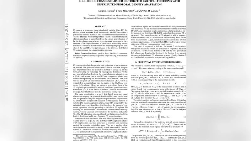
We present a consensus-based distributed particle filter (PF) for wireless sensor networks. Each sensor runs a local PF to compute a global state estimate that takes into account the measurements of all sensors. The local PFs use the joint (all-sensors) likelihood function, which is calculated in a distributed way by a novel generalization of the likelihood consensus scheme. A performance improvement (or a reduction of the required number of particles) is achieved by a novel distributed, consensus-based method for adapting the proposal densities of the local PFs. The performance of the proposed distributed PF is demonstrated for a target tracking problem.

💡 Research Summary

This paper proposes a novel consensus‑based distributed particle filter (DPF) tailored for wireless sensor networks (WSNs) where each sensor runs its own local particle filter yet produces a global state estimate that incorporates measurements from all sensors. The key contributions are twofold. First, the authors generalize the likelihood consensus (LC) scheme so that it is no longer limited to additive Gaussian measurement noise or exponential‑family likelihoods. By approximating each sensor’s log‑likelihood with a finite‑dimensional basis expansion, log f(zₙ,ₖ|xₙ) ≈ Σ₍ᵣ₎ αₙ,ₖ,ᵣ(zₙ,ₖ) ϕₙ,ᵣ(xₙ), the coefficients αₙ,ₖ,ᵣ are computed locally via least‑squares fitting on the particles generated by the filter. The coefficients are then summed across the network using standard average‑consensus iterations, yielding global coefficients aₙ,ᵣ(zₙ)=Σₖαₙ,ₖ,ᵣ(zₙ,ₖ). Because aₙ,ᵣ(zₙ) are scalar values independent of the unknown state, they can be exchanged efficiently among neighboring nodes. Each sensor can reconstruct an approximation of the joint likelihood (JLF) as ˜f(zₙ|xₙ)=exp(Σ₍ᵣ₎ aₙ,ᵣ(zₙ) ϕₙ,ᵣ(xₙ)), which can be evaluated for any xₙ without further communication. This generalized LC works for arbitrary nonlinear, non‑Gaussian measurement models and scales well with high‑dimensional measurements because the communication load depends only on the number of basis functions and consensus iterations, not on measurement dimension.

The second major contribution is a distributed proposal density (PD) adaptation scheme. In particle filtering, the choice of proposal density q(xₙ|zₙ) critically affects performance; a poorly chosen q leads to weight degeneracy and requires many particles. The authors construct a “pre‑distorted” local pseudo‑posterior at each sensor: ˜f(xₙ|z₁:ₙ₋₁, zₙ,ₖ)=f(zₙ,ₖ|xₙ)·𝒩(xₙ; μ′ₙ,ₖ, K C′ₙ,ₖ), where μ′ₙ,ₖ and C′ₙ,ₖ are the Gaussian approximations of the predicted posterior obtained in the local PF, and K is the number of sensors. This pseudo‑posterior is approximated by a Gaussian 𝒩(xₙ; μ̃ₙ,ₖ, C̃ₙ,ₖ) using a standard Gaussian update (e.g., EKF or UKF) with the local measurement. The product of all K pseudo‑posteriors yields, up to a normalization constant, the true global posterior f(xₙ|z₁:ₙ). By exploiting the closed‑form product of Gaussian densities, the global proposal density q(xₙ;zₙ)=𝒩(xₙ; μₙ, Cₙ) can be expressed as

 μₙ = Cₙ Σₖ C̃ₙ,ₖ⁻¹ μ̃ₙ,ₖ,  Cₙ = (Σₖ C̃ₙ,ₖ⁻¹)⁻¹.

The required sums Σₖ C̃ₙ,ₖ⁻¹ μ̃ₙ,ₖ and Σₖ C̃ₙ,ₖ⁻¹ are computed in a distributed fashion via consensus. Consequently, each sensor obtains a globally informed proposal density that reflects all measurements, leading to a dramatic reduction in the number of particles needed for a given accuracy.

The complete algorithm proceeds as follows at each time step n:

1. Resampling of the previous particle set at each sensor.
2. Prediction: draw temporary particles from the state‑transition model and compute Gaussian approximations (μ′ₙ,ₖ, C′ₙ,ₖ) of the predicted posterior.
3. PD Adaptation: locally update the pseudo‑posterior using the measurement, obtain (μ̃ₙ,ₖ, C̃ₙ,ₖ), then run consensus to compute the global μₙ and Cₙ.
4. Sampling: draw J particles from the global proposal density q(xₙ;zₙ).
5. Generalized LC: each sensor computes its basis‑expansion coefficients αₙ,ₖ,ᵣ from the particles and its measurement, then runs R parallel consensus processes (one per basis function) to obtain the global coefficients aₙ,ᵣ(zₙ).
6. Weight Update: evaluate the approximated joint likelihood ˜f(zₙ|xₙ) using (μₙ, Cₙ) and the global coefficients, then compute particle weights wₙ,ₖ^(j) = γ ˜f(zₙ|xₙ^(j)) f(xₙ^(j)|xₙ₋₁^(j))/q(xₙ^(j);zₙ).
7. State Estimate: form the weighted mean as the MMSE estimate.

The communication overhead consists of I·R real numbers per sensor for the LC (I = number of consensus iterations, R = number of basis functions) and I·