Fixed-delay Events in Generalized Semi-Markov Processes Revisited

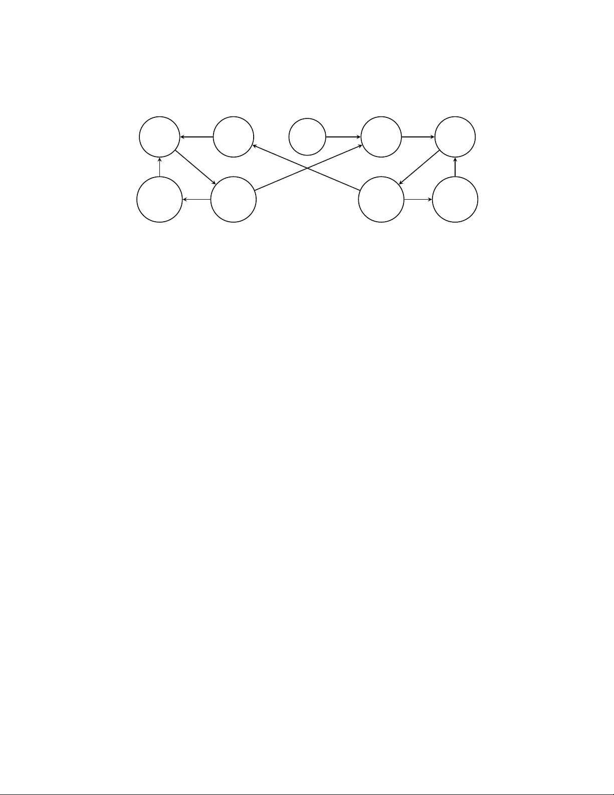
Fixed-delay Events i n Generalized Semi-Mark ov Pr ocesses Re visited ⋆ T omáš Brázdil, Jan Kr ˇ cál, Jan K ˇ retínský ⋆⋆ , and V ojt ˇ ech ˇ Rehák Faculty of Informatics, Masaryk Uni ve rsity , Brno, Czech Republic {brazdil, krcal, jan.kretinsk y , rehak}@ﬁ.muni.cz Abstract. W e study long run av erage b ehav ior of ge neralized semi-Mark ov pro - cesses with both ﬁx ed-delay e ven ts as well as v ariable-delay even ts. W e show that allowin g two ﬁ xed-d elay e vents and one v ariable-delay ev ent may cause an unsta- ble behavior of a GSMP . In particular , we show that a frequency of a given state may not be deﬁned for almost all runs (or more generally , an in variant measure may not exist). W e use this observation to disprove sev eral results from litera- ture. Next we study GSMP with at most one ﬁxed-delay ev ent combined with an arbitrary number of variab le-delay e vents. W e prove that such a GSMP alwa ys possesses an in variant measure which means that the frequencies of states are alway s well deﬁned and we provide algorithms for approximation of these fre- quencies. Additionally , we sho w that the positive results remain valid ev en if we allow an a rbitrary number of reasonably restricted ﬁxed-delay e vents. 1 Intr o duction Generalized semi-Ma rkov proce sses ( GSMP), introd uced by Matthes in [22], are a stan- dard model for d iscrete-event stochastic systems. Such a system operates in con tinuous time and reacts, by changing its state, to occurren ces of e vents. Each ev ent is assigned a random delay after wh ich it o ccurs; state tran sitions may b e ran domized as well. When- ev er the system r eacts to an event, new events may b e sch eduled and pendin g events may be discarded. T o get some intuition, imagine a simple commun ication model in wh ich a server sends messages to sev eral clients asking th em to rep ly . The reactio n of each client may be randomly delayed, e.g., due to latency of commun ication links. Whene ver a re- ply comes from a client, th e server c hanges its state (e.g., by upd ating its d atabase of aliv e clients o r b y send ing anoth er message to the client) a nd th en waits f or th e rest of the replies. Su ch a m odel is u sually extended by allowing the ser ver to time-ou t and to take an appr opriate action , e.g., demand replies from the remainin g clien ts in a mor e urgent w ay . Th e time-out can be seen as another e vent which has a ﬁxed delay . More f ormally , a GSMP con sists of a set S of states and a set E of events. Each state s is a ssigned a set E ( s ) of events scheduled in s . In tuiti vely , each event in E ( s ) is assigned a positive real nu mber r epresenting th e amoun t of time wh ich elapses befor e ⋆ The authors are supported by the Institute for T heoretical Computer Science, project No. 1M0545, the Czech Science Found ation, grant No. P202 / 10 / 1469 (T . Brázdil, V . ˇ Rehák) and No. 102 / 09 / H042 (J. Kr ˇ cál), and Brno PhD T alent Financial Aid (J. K ˇ retínský). ⋆⋆ On leav e at TU München , Boltzmannstr . 3, Garching, German y . the event o ccurs. Note th at se veral ev ents may occur at the same time. Onc e a set of ev ents E ⊆ E ( s ) occurs, th e system makes a transition to a new state s ′ . The state s ′ is rand omly chosen accor ding to a ﬁxed distrib ution which d epends only o n the state s and the set E . In s ′ , the old events of E ( s ) r E ( s ′ ) are discarded, each inherited event of ( E ( s ′ ) ∩ E ( s )) r E remains scheduled to the same point in the future, an d ea ch new event of ( E ( s ′ ) r E ( s )) ∪ ( E ( s ′ ) ∩ E ) is newly scheduled accord ing to its given pr obability distribution. In order to deal with GSMP in a r igorous way , o ne has to im pose some r estrictions on the distributions of delays. Standa rd mathem atical literature, such as [14,15], usually considers GSMP with c ontinuou sly distributed delays. This is certainly a limitation, as some systems with ﬁxed time delays ( such as time- outs o r pr ocessor ticks) cannot be faithfully mode led using only con tinuously distributed delay s. W e show some exam - ples where ﬁxed delays exhibit qualitatively d i ﬀ erent behavior than a ny con tinuously distributed approximation. In this paper we consider t he following tw o types of e vents: – variable-d elay : th e delay o f the e vent is randomly distributed ac cording to a proba- bility den sity function which is continu ous an d positiv e either on a bounded inter val [ ℓ, u ] or on an unbou nded interval [ ℓ, ∞ ); – ﬁxed-d elay : the delay is set to a ﬁxed v alue with probability one. The desired behavior o f systems modeled using GSMP can be speciﬁed by various means. One is often interested in long- run behavior such as mean response time, f re- quency of error s, etc. (see, e.g., [1]). For examp le, in the above commun ication model, one may b e interested in av erage response time o f clients or in average time in whic h all clients e ventually reply . Several model indepen dent forma lisms hav e bee n devised for expressing such properties of co ntinuou s time systems. For examp le, a well k nown temporal logic CSL contain s a steady state op erator expressing f requency o f states satisfying a giv en subfor mula. In [9], we pr oposed to specify long- run behavior of a continuo us-time process using a timed autom aton wh ich o bserves run s o f the p rocess, and measure the frequen cy o f locations of the automaton. In this p aper we consider a standard perfo rmance measure , the freq uency of states of the GSMP . T o be more speciﬁc, let us ﬁx a state ˚ s ∈ S . W e d eﬁne a random variable d which to every run assigns the (discre te) frequ ency of visits to ˚ s on the r un, i.e. the ratio of the nu mber of tr ansitions entering ˚ s to the n umber of all transitions. W e also deﬁne a r andom v ariable c which gives timed frequency of ˚ s , i.e. the ratio of the amo unt of time spent in ˚ s to th e a mount of time spent in all states. T e chnically , b oth variables d and c are deﬁned as limits o f the co rrespond ing ra tios on preﬁxes of the r un that are p rolong ed ad inﬁn itum. Note that the limits may n ot b e deﬁne d fo r some r uns. For example, con sider a run which alternates b etween ˚ s and an other state s ; it spen ds 2 time unit in ˚ s , then 4 in s , then 8 in ˚ s , then 16 in s , etc. Such a ru n does no t h av e a limit ratio between time sp ent in ˚ s a nd in s . W e say that d (or c ) is well-deﬁn ed for a run if the limit r atios exist for this run . Our goal is to characterize stable system s that have the variables d and c well-deﬁned for almost a ll run s, and to analyze th e p robability distributions of d and c on these stable systems. As a working example of GSMP with ﬁxed-delay ev ents, we present a simpliﬁed protoco l for time synchron ization. Using the variable c , we sho w how to measure relia- bility of the p rotocol. V ia m essage exchange, the protocol sets and keeps a client clock 2 Init { query , stable _ d } Q-sent { re s pon se , round tr i p _ d , stable _ d } R-recvd { sync } Idle { stable _ d , polling _ d } Init’ { query } Q-sent’ { re s pon se , round tr i p _ d } query re s pon se sync round tr i p _ d query re s pon se round tr i p _ d polling _ d stable _ d stable _ d Fig. 1. A GSMP model of a clock synchronization protocol. B elo w each state label, we list the set of scheduled e vents. W e only display transitions that c an tak e place with n on-zero p robability . su ﬃ ciently close to a server clo ck. Each message exchang e is initialized by the client asking th e ser ver for the cur rent time, i.e. sendin g a query message. Th e server adds a timestamp into th e message an d send s it b ack as a r espo nse . Th is q uery-r esponse ex- change provides a reliable data for synchr on ization a ction i f it is realized within a giv en r ound -trip delay . Otherwise, the client has to rep eat the procedu re. After a success, the client is considered to be synchro nized until a gi ven stable-time d elay elap ses. Since the aim is to keep the clo cks syn chronized all the time , the client r estarts the synchron iza- tion process soone r , i.e. after a given p olling delay that is shorter than the stable-time delay . Notice that the clien t gets desyn chronized whenever several unsuccessful syn - chroniza tions oc cur in a row . Our g oal is to measure the portion of the time wh en th e client clock is not synchro nized. Figure 1 shows a GSMP model of this protoco l. The delays speciﬁed in the proto - col ar e modeled using ﬁxed-d elay events ro und tr i p _ d , st able _ d , and p olling _ d while actions are mod eled b y variable-delay events quer y , r e s pon se , and sync . No te that if the stable-time runs out before a fast enoug h respon se arrives, the systems moves into primed states denoting it is not synchron ized at the moment. Thus, c ( Init’ ) + c ( Q-sent’ ) expresses the portion of the time when the client clock is not synchronized . Our contrib ut ion. So far, GSMP were mostly stud ied with v ar iable-delay e vents o nly . There ar e a fe w e x ceptions such as [4,3,8,2] but they often co ntain erro neous statements due to pr esence of ﬁ xed-delay events. Our g oal is to study the e ﬀ ect of mix ing a number of ﬁxed-delay e vents with an arbitrary amoun t of variable-delay ev ents. At the beginn ing we give a n example of a GSMP with two ﬁxed-d elay ev ents fo r which it is not true that the variables d and c are well-deﬁned fo r almost all runs. W e also d isprove some crucial statemen ts of [ 3,4]. In particular, we show an example of a GSMP which rea ches on e of its states with pro bability less than one ev en thou gh the algo rithms o f [3,4] retu rn the p robability one. The mistake of these alg orithms is fundam ental as they neglect th e possibility of unstable behavior of GSMP . Concernin g positi ve results, we show that if ther e is at most on e ﬁxed-d elay e vent, then bo th d an d c ar e almo st surely well-deﬁn ed. This is true even if we allow an a rbi- trary number of reasonably restricted ﬁxed-d elay events. W e also sho w h ow to approx i- 3 mate distribution functio ns of d and c . T o be more speciﬁc, we show th at for GSMP with at most one unrestricted and a n a rbitrary numbe r of restricted ﬁxed-delay events, both variables d and c ha ve ﬁnite ranges { d 1 , . . . , d n } and { c 1 , . . . , c n } . Moreover , all v alue s d i and c i and probabilities P ( d = d i ) and P ( c = c i ) can be e ﬀ ectively approxim ated. Related work. Ther e are two m ain ap proaches to the analysis o f GSMP . On e is to r e- strict the amount of events or typ es of their distributions an d to solve the pr oblems using symbolic metho ds [ 8,2,20]. The other is to estimate the values of interest using simu- lation [26,14,15]. Concern ing the ﬁrst appro ach, time-bo unded reachab ility has bee n studied in [2] where the authors restricted the delays of events to so c alled expo lyno- mial d istributions. T he same autho rs also studie d reach ability probab ilities o f GSMP where in each transition at most on e event is in herited [ 8]. Fu rther, the wid ely studied formalisms o f semi-M arkov p rocesses (see, e .g., [19,9]) and continu ous-time Markov chains (see, e.g., [6,7]) are both subclasses of GSMP . As for the second app roach, GSMP are studied by mathematician s as a stan- dard mod el fo r discrete event simulatio n an d Markov ch ains Monte Carlo (see, e.g., [13,16,24]). Our work is stron gly related to [1 4,15] wh ere the long -run average be havior of GSMP with variable-delay events is studied. Under re lati vely standar d assumption s the stochastic p rocess gene rated b y a GSMP is shown to be ir reducible and to possess an in variant measure . In such a case, the variables d an d c are almost surely co nstant. Be- side the theoretical results, there exist tools that employ simulation for model checking (see, e.g., [26,10]). In addition, GSMP ar e a p roper subset of stochastic automata, a m odel of co ncur- rent systems (see, e.g., [11]). Further, as shown in [15], GSMP have the same modeling power as stochastic Petri nets [21]. The formalism of determ inistic and stochastic Petri nets (DSPN) intro duced by [20] adds deterministic transition s – a counterp art of ﬁxed- delay events. The author s restricted the model to at most one determin istic tr ansition enabled at a tim e and to expo nentially distributed timed transition s. For th is restricted model, the authors proved existence of a steady state distribution an d p rovided an al- gorithm for its computation . Howe ver, th e methods inherently rely o n the prope rties of the exponential distribution and cannot be extended to o ur setting wi th general variable delays. DSPN have been extended b y [12,18] to allow arbitrarily m any deterministic transitions. The au thors provide algorithm s f or steady-state analysis of DSPN that were implemented in the tool DSPNExpress [17], but do not discuss under which conditions the steady-state distributions e x ist. 2 Pr eliminaries In this p aper, the sets o f all p ositi ve integers, non-negative integers, real n umbers, pos- iti ve real nu mbers, and non-n egati ve real number s are d enoted b y N , N 0 , R , R > 0 , and R ≥ 0 , respectively . For a real number r ∈ R , int ( r ) denotes its integral part, i.e. the largest integer smaller than r , and fr ac( r ) d enotes its fractio nal pa rt, i. e. r − in t( r ) . L et A be a ﬁnite o r co untably inﬁnite s et. A pr o bability distribution on A is a function f : A → R ≥ 0 such that P a ∈ A f ( a ) = 1. The set of all distributions on A is den oted by D ( A ). 4 A σ -ﬁeld over a set Ω is a set F ⊆ 2 Ω that in cludes Ω an d is closed unde r comple- ment and co untable union. A measurable space is a pair ( Ω, F ) where Ω is a set called sample space an d F is a σ -ﬁeld over Ω whose elemen ts are called measurable sets . Giv en a measurable spac e ( Ω, F ), we say th at a fu nction f : Ω → R is a ran dom vari- able if the in verse image of any real interv al is a measurable set. A pr obab ility measur e over a mea surable space ( Ω, F ) is a function P : F → R ≥ 0 such that, for each c ountable collection { X i } i ∈ I of pairwise disjoin t ele ments of F , we h av e P ( S i ∈ I X i ) = P i ∈ I P ( X i ) and, m oreover , P ( Ω ) = 1. A pr obability space is a tr iple ( Ω, F , P ), where ( Ω, F ) is a measurable space an d P is a pro bability measure over ( Ω, F ). W e say that a proper ty A ⊆ Ω holds for almost all elements of a measurable set Y if P ( Y ) > 0 , A ∩ Y ∈ F , and P ( A ∩ Y | Y ) = 1 . Alternativ ely , we say that A h olds almost sur ely for Y . 2.1 Generalized semi-Marko v processes Let E b e a ﬁnite set of events . T o every e ∈ E we associate the lower b ound ℓ e ∈ N 0 and th e up per bou nd u e ∈ N ∪ {∞} of its delay . W e say that e is a ﬁxed -delay ev ent if ℓ e = u e , an d a variab le-delay event if ℓ e < u e . Fur thermore , we say that a variable- delay event e is b ounded if u e , ∞ , and u nboun ded , otherwise. T o each variable-delay ev ent e we a ssign a density functio n f e : R → R such that R u e ℓ e f e ( x ) dx = 1 . W e assume f e to be p ositi ve an d co ntinuou s on the w hole [ ℓ e , u e ] or [ ℓ e , ∞ ) if e is bo unded or unbou nded, respectiv ely , and ze ro else where. W e re quire th at f e have ﬁnite expected value, i.e. R u e ℓ e x · f e ( x ) dx < ∞ . Deﬁnition 1. A gener alized semi-Markov process is a tuple ( S , E , E , Succ , α 0 ) wher e – S is a ﬁnite set of states , – E is a ﬁnite set of events , – E : S → 2 E assigns to each state s a set of events E ( s ) , ∅ scheduled to occur in s, – Succ : S × 2 E → D ( S ) is the successor function, i.e. assign s a p r obab ility dis- tribution spec ifying the successor state to each state and set of events that occur simultaneou sly in this state, and – α 0 ∈ D ( S ) is the in itial distrib ution . A conﬁgu ration is a pair ( s , ν ) wh ere s ∈ S and ν is a valua tion which assigns to ev ery ev ent e ∈ E ( s ) the amou nt of time that elap sed since th e ev ent e was schedu led. 1 For c on venience, we deﬁne ν ( e ) = ⊥ whenever e < E ( s ), and we deno te by ν ( △ ) the amount of time spent in the previous conﬁgur ation (initially , we put ν ( △ ) = 0). When a set of events E o ccurs and the proce ss moves fro m s to a state s ′ , th e valuation of old events of E ( s ) r E ( s ′ ) is discard ed to ⊥ , the valuation of each in herited ev ent of ( E ( s ′ ) ∩ E ( s )) r E is increased by the time spen t in s , an d th e valuation of each new ev ent of ( E ( s ′ ) r E ( s )) ∪ ( E ( s ′ ) ∩ E ) is set to 0. W e illustrate the dynamics of GSMP on the examp le of Figu re 1. Let the bound s of the ﬁxed-delay events r ound t r i p _ d , polling _ d , an d stable _ d be 1 Usually , the valuation is deﬁned t o store the ti me left before the eve nt appears. Howe ver , our deﬁnition is equi valent and more con venient for the general setting where both bounded and unboun ded e vents app ear . 5 1, 90, and 100, respectively . W e start in the state Id le , i.e. in the conﬁgu- ration ( Id le , (( polling _ d , 0) , ( stable _ d , 0) , ( △ , 0) )) denoting that ν ( polling _ d ) = 0, ν ( st able _ d ) = 0 , ν ( △ ) = 0, and ⊥ is assigned to all other ev ents. After 90 time units, the event p olling _ d occ urs an d we move to ( Init , ( ( quer y , 0) , ( stable _ d , 90) , ( △ , 90))). Assume that the e vent query occurs in the state Init after 0 . 6 time units and we move to ( Q-sent , (( r e s pon se , 0) , ( r ound t ri p _ d , 0) , ( stab le _ d , 90 . 6) , ( △ , 0 . 6))) an d so forth. A for mal seman tics of GSMP is usually deﬁne d in ter ms of g eneral state-space Markov chains (GSSMC, see, e.g., [23]). A GSSMC is a stoch astic process Φ over a measurable state-spa ce ( Γ , G ) whose d ynamics is de termined by an in itial measure µ on ( Γ , G ) and a transition kernel P which speciﬁes on e-step transition prob abilities. 2 A given GSMP induc es a GSSMC whose state- space consists o f all conﬁgur ations, the initial measur e µ is ind uced by α 0 in a natura l way , an d th e tr ansition kernel is determined by the dynamics of GSMP described above. Formally , – Γ is the set o f all conﬁguratio ns, and G is a σ -ﬁeld over Γ ind uced by th e discre te topolog y over S and the Borel σ -ﬁeld over the s et of all v aluations; – the initial measure µ allows to start in c onﬁguratio ns with z ero valuation o nly , i.e. for A ∈ G we have µ ( A ) = P s ∈ Zer o ( A ) α 0 ( s ) wher e Zer o ( A ) = { s ∈ S | ( s , 0 ) ∈ A } ; – the transition kern el P ( z , A ) d escribing the pr obability to move in on e step fro m a conﬁg uration z = ( s , ν ) to any conﬁgura tion in a set A is deﬁned as f ollows. It su ﬃ ces to co nsider A of the for m { s ′ } × X where X is a measur able set of valuations. Let V and F be th e sets of variable-delay and ﬁxed-delay e vents, respectively , that are scheduled in s . Let F ′ ⊆ F be the set of ﬁxed-de lay events that can occur as ﬁrst among the ﬁxed-delay e vent enable d in z , i.e. that have in ν the m inimal remaining time u . Note th at two variable-d elay events occu r simultan eously with probab ility zero. Hence, we consider all combinatio ns of e ∈ V and t ∈ R ≥ 0 stating that P ( z , A ) =        P e ∈ V R ∞ 0 Hit( { e } , t ) · W in( { e } , t ) dt if F = ∅ P e ∈ V R u 0 Hit( { e } , t ) · W in( { e } , t ) dt + Hit( F ′ , u ) · W in( F ′ , u ) other wise, where the term Hit( E , t ) den otes the con ditional p robability o f h itting A u nder the condition tha t E o ccurs at time t and th e term W in( E , t ) deno tes the p robability (density) of E occur ring at time t . Forma lly , Hit( E , t ) = Su cc( s , E )( s ′ ) · 1 [ ν ′ ∈ X ] where 1 [ ν ′ ∈ X ] is the indicator function and ν ′ is the valuation after the transition, i.e. ν ′ ( e ) is ⊥ , o r ν ( e ) + t , or 0 for e ach o ld, or inher ited, o r new event e , respec- ti vely; and ν ′ ( △ ) = t . The most com plicated par t is the deﬁnition of Win( E , t ) which intuitively corr esponds to the prob ability that E is the set of ev ents “win ning” the competition am ong the events scheduled in s at time t . First, we deﬁne a “shifted” density function f e | ν ( e ) that takes into account t hat the time ν ( e ) has already elapsed . Formally , for a variable-delay e vent e and any elapsed time ν ( e ) < u e , we deﬁne f e | ν ( e ) ( x ) = f e ( x + ν ( e )) R ∞ ν ( e ) f e ( y ) dy if x ≥ 0. 2 Precisely , transition kernel is a function P : Γ × G → [0 , 1] such that P ( z , · ) is a probability measure ov er ( Γ , G ) for each z ∈ Γ ; and P ( · , A ) is a measurable function for each A ∈ G . 6 Otherwise, we d eﬁne f e | ν ( e ) ( x ) = 0. The denom inator scales the fu nction so that f e | ν ( e ) is again a density function . Finally , W in( E , t ) =              f e | ν ( e ) ( t ) · Q c ∈ V \ E R ∞ t f c | ν ( c ) ( y ) d y if E = { e } ⊆ V Q c ∈ V R ∞ t f c | ν ( c ) ( y ) d y if E = F ′ ⊆ F 0 otherwise. A run of the Markov ch ain is an inﬁnite sequ ence σ = z 0 z 1 z 2 · · · of con ﬁguration s. The Markov c hain is deﬁned on th e pr obability space ( Ω, F , P ) where Ω is the set of all runs, F is the pr oduct σ -ﬁeld N ∞ i = 0 G , and P is the un ique probability measure s uch that for ev ery ﬁnite sequence A 0 , · · · , A n ∈ G we have that P ( Φ 0 ∈ A 0 , · · · , Φ n ∈ A n ) = Z z 0 ∈ A 0 · · · Z z n − 1 ∈ A n − 1 µ ( dz 0 ) · P ( z 0 , dz 1 ) · · · P ( z n − 1 , A n ) where each Φ i is the i -th projection of an element in Ω ( the i -th conﬁguration of a run). Finally , we deﬁne an m -step tran sition kern el P m inductively as P 1 ( z , A ) = P ( z , A ) and P i + 1 ( z , A ) = R Γ P ( z , d y ) · P i ( y , A ). 2.2 Frequency measur es Our attention fo cuses on frequen cies of a ﬁxed state ˚ s ∈ S in the runs of the Markov chain. Let σ = ( s 0 , ν 0 ) ( s 1 , ν 1 ) · · · be a run . W e de ﬁne d ( σ ) = lim n →∞ P n i = 0 δ ( s i ) n c ( σ ) = lim n →∞ P n i = 0 δ ( s i ) · ν i + 1 ( △ ) P n i = 0 ν i + 1 ( △ ) where δ ( s i ) is eq ual to 1 when s i = ˚ s , and 0 otherwise. W e r ecall that ν i + 1 ( △ ) is the time spent in state s i before movin g to s i + 1 . W e say that the random variable d or c is well-deﬁned for a r un σ if the co rrespond ing limit e xists for σ . T hen, d cor respond s to the frequency of discrete visits to the state ˚ s and c co rrespond s to the ratio of ti me spent in the state ˚ s . 2.3 Region graph In ord er to state the results in a simp ler way , we in troduce the r e gio n gr aph , a standa rd notion from the area of timed automata [5]. It is a ﬁnite partition of the uncou ntable set of conﬁgur ations. F irst, we deﬁne the region relation ∼ . For a , b ∈ R , we say that a and b agree on inte gral part if int( a ) = int( b ) an d neither o r both a , b ar e integers. Further, we set the boun d B = ma x  { ℓ e , u e | e ∈ E} \ {∞}  . Finally , we put ( s 1 , ν 1 ) ∼ ( s 2 , ν 2 ) if – s 1 = s 2 ; – for all e ∈ E ( s 1 ) we h av e that ν 1 ( e ) and ν 2 ( e ) ag ree on integral parts o r are bo th greater than B ; – for all e , f ∈ E ( s 1 ) with ν 1 ( e ) ≤ B and ν 1 ( f ) ≤ B we have th at frac( ν 1 ( e )) ≤ frac( ν 1 ( f ) ) i ﬀ f rac( ν 2 ( e )) ≤ fr ac( ν 2 ( f ) ). 7 Init { p } 2 C-waiting { p , t } 2 Consuming { p , c } 2 Consuming T ransporting { p , t , c } 2 Bu ﬀ ering Consuming { p , c } 1 C-waiting { p , t } 1 Consuming { p , c } 1 Consuming T ransporting { p , t , c } 1 Bu ﬀ ering Consuming { p , c } p t p t c c t p t c c Fig. 2. A GSMP of a producer -consumer system. The ev ents p , t , and c model that a packet production, transport, and consumption i s ﬁ nished, respecti vely . Below each state label, t here is the set of scheduled ev ents. The ﬁxed-delay e vents p and c have l p = u p = l c = u c = 1 and the uniformly distributed v ariable-delay even t t has l t = 0 and u t = 1. Note that ∼ is a n equivalence with ﬁn ite index. The equiv alence classes of ∼ are called r egions . W e deﬁne a ﬁ nite r egion g raph G = ( V , E ) where the s et of vertices V is the set of re gions and fo r e very p air of regions R , R ′ there is an edge ( R , R ′ ) ∈ E i ﬀ P ( z , R ′ ) > 0 for some z ∈ R . The c onstruction is co rrect because all states in the same region have the same one-step qualitative behavior (for details, see Appendix B.1). 3 T wo ﬁxed-delay events Now , we explain in more detail what p roblems can be caused by ﬁxed-d elay events. W e start with an example o f a GSMP with two ﬁxed-delay events for which it is not true that the variables d an d c are well-d eﬁned for almost all runs. Then we sho w some other examples o f GSMP with ﬁxed-delay events th at disprove some results fr om litera ture. In the next section, we provide p ositiv e results when the n umber and type of ﬁxed-delay ev ents are limited. When the frequencies d and c are not well-deﬁned In Figure 2, we sh ow an example o f a GSMP with two ﬁxed-delay events a nd one variable-delay event for which it is not true th at th e variables d and c are well-deﬁned for almost all r uns. It mo dels the following pr oducer-consume r system. W e u se three compon ents – a produ cer , a tra nsporter and a consumer o f p ackets. The co mponen ts work in parallel but each compo nent can pr ocess (i.e. pr oduce, tran sport, or co nsume) at most one packet at a time. Consider the following time requ irements: each packet p roductio n takes exactly 1 time unit, each transpo rt takes at most 1 tim e unit, and each consump tion takes again exactly 1 time unit. As there a re no lim itations to block the producer, it is working for all the time a nd new packets are produ ced precisely each time unit. As the tran sport takes shorter time than the productio n, every n e w packet is im mediately taken by the trans- porter and no bu ﬀ er is needed at this place. When a p acket arri ves to the consumer, the consump tion is started immediately if the consum er is waiting; otherwise, the packet 8 Init { p } C-waiting { p , t , t ′ } Consuming { p , c } Consuming T ransporting { p , t , c } Bu ﬀ ering Consuming { p , c } Sink { p } p t ′ p t p t c c Fig. 3. A GS MP with t wo ﬁ xed-d elay ev ents p and c (with l p = u p = l c = u c = 1), a uniformly distributed v ariable-delay ev ents t , t ′ (with l t = l t ′ = 0 and u t = u t ′ = 1). is stored into a bu ﬀ er . When the co nsumption is ﬁn ished and the bu ﬀ er is empty , the consumer waits; otherwise, a new consumption starts immediately . In the GSMP in Figure 2, th e con sumer has two mod ules – o ne is in o peration and the o ther idles at a time – when th e con sumer enters the waiting state, it switches the modules. The labels 1 and 2 denote which module of the consumer is in operation . One can easily observe that the consumer enters the w a iting state (and switches the modules) if an d only if th e curren t tran sport takes more time th an it h as ev er ta ken. As the tran sport time is bound ed b y 1, it gets h arder and ha rder to break th e rec ord. As a result, the sy stem stays in the cu rrent modu le o n average f or longer time than in the p revious module. Therefor e, du e to the successively p rolong ing stay s in the mod - ules, the fr equencies for 1-states an d 2-states oscillate. For precise computatio ns, see Append ix A.1. W e co nclude the above o bservation by the following theorem. Theorem 1. There is a GSMP (with two ﬁxed -delay events and on e v ariable-dela y event) for which it is not true that the variables c and d ar e almost surely w ell-deﬁned . Counterexamples In [3,4] there are algorithms for GSMP model checkin g based on the region co nstruc- tion. They rely on tw o crucial statements of the papers: 1. Almost all runs e nd i n some o f the bottom strongly co nnected componen ts (BSCC) of the region graph. 2. Almost all runs entering a BSCC visit all regions of the compone nt inﬁn itely often. Both of these stateme nts are true for ﬁnite state Markov chains. In th e following, we show that neither of them has to be valid for region graphs of GSMP . Let us consider the GSMP depicted in Figu re 3. This is a p roducer-consu mer mo del similar to the previous example but we h av e only one module of the co nsumer here . Again, entering th e state C-waiting in dicates that the current transpor t takes more time than it has ev er taken. In the state C-waiting , an additional e vent t ′ can occur and move the system in to a state Sin k . One can in tuiti vely obser ve that we enter the state C-waiting less and less o ften and stay ther e for shorter an d sho rter time. Hence, the proba bility 9 that the e vent t ′ occurs in th e state C-waitin g is decreasing during th e r un. For precise computatio ns proving the follo wing claim, see Appendix A.2. Claim. The probab ility to reach Sink fro m Init is strictly less than 1. The above claim directly implies the following theorem thus disproving statement 1. Theorem 2. There is a GSMP (with two ﬁxed-d elay and two va riable d elay events) wher e th e pr obab ility to r each any BSCC of the r egion gr aph is strictly smaller than 1. Now co nsider in Figure 3 a tra nsition und er the event p f rom the state S ink to the state Init instead of the self-loop. T his turns the wh ole region grap h into a single BSCC. W e pr ove that the state S ink is almost surely visited on ly ﬁnitely often. I ndeed, let p < 1 be the o riginal proba bility to reach S ink g uaranteed by th e claim ab ove. The probab ility to reach Sink from S ink ag ain is also p as th e only tran sition leading fr om Sink enters th e initial conﬁgur ation. T herefor e, the prob ability to reach Sink inﬁnitely often is lim n →∞ p n = 0. This proves the f ollowing theo rem. Hence , the statem ent 2 of [3,4] is disproved, as well. Theorem 3. There is a GSMP (with two ﬁxed-d elay and two va riable d elay events) with str o ngly connecte d r egion graph a nd with a r e gio n th at is reac hed inﬁ nitely often with pr oba bility 0 . 4 Single-ticking GSMP First of all, moti vated by the previous c ounterexamp les, we identify the beha vior of the ﬁxed-delay ev ents that m ay cause d and c to be u ndeﬁned. The problem lies in ﬁxed- delay events that can im mediately schedu le themselves wh enev er they occur; such an ev ent can occur periodically like tickin g of clocks. In the example of Figure 3, ther e are two such e vents p and c . The phase di ﬀ er ence of their t icking gets smaller and smaller, causing the unstable behavior . For two ﬁxed-delay events e and e ′ , we say that e causes e ′ if there are states s , s ′ and a set of e vents E such that Succ( s , E )( s ′ ) > 0, e ∈ E , and e ′ is newly sched uled in s ′ . Deﬁnition 2. A GS MP is called sing le-ticking if either ther e is no ﬁxed -delay event or the r e is a strict total o r der < on ﬁxed- delay events with the least element e (called ticking event) such that whenever f causes g then either f < g or f = g = e. From now on we restrict to single-ticking GSMP and prove our main positive resu lt. Theorem 4. In single-ticking GS MP , th e random variables d and c ar e well-deﬁned for almost every run and a dmit on ly ﬁn itely man y va lues. Precisely , almost every run r eaches a BSCC of the r egion gr a ph and for each BSCC B ther e are values d , c ∈ [0 , 1 ] such that d ( σ ) = d and c ( σ ) = c for almo st all runs σ that r each the BSCC B. The rest of this section is devoted to the proof of Th eorem 4. Fir st, we show that almost all run s en d up trapp ed in som e BSCC of the r egion g raph. Seco nd, we solve the proble m while restricting to runs th at start in a BSCC (as the initial part of a r un outside of any BSCC is not relev ant for the long ru n a verage beh a vior). W e sho w that in a BSCC, the variables d and c ar e almost surely c onstant. The secon d part of th e proo f relies on several stan dard results from the theory of general state space Markov chains. Formally , the proo f follows from Propositions 1 and 2 stated below . 10 4.1 Reaching a BSCC Proposition 1. In single-ticking GSMP , almost every run r eaches a BSCC o f the r egion graph. The proof uses similar methods as the proof in [4]. By deﬁnition, the process moves along the ed ges of the region graph. From ev ery r egion, there is a m inimal path thr ough the r egion graph into a BSCC, let n be th e max imal length o f all such p aths. Hence, in at m ost n steps th e pro cess reach es a BSCC with p ositiv e probab ility from any conﬁg- uration. Observe that if this prob ability w as bound ed from below , we would e ventually reach a BSCC from any conﬁg uration almost surely . Howev er , this p robability can be arbitrarily small. Consider th e fo llowing example with ev ent e un iform on [0 , 1] and ev ent f u niform on [2 , 3]. In an intuitive notation, let R be the r egion [0 < e < f < 1 ]. What is the pro bability th at the ev ent e occurs after the elap sed tim e of f reaches 1 (i.e. that the r egion [ e = 0 ; 1 < f < 2] is r eached)? For a conﬁg uration in R with val- uation (( e , 0 . 2) , ( f , 0 . 7)) the pr obability is 0 . 5 but f or ano ther conﬁgu ration in R with (( e , 0 . 2) , ( f , 0 . 21) ) it is only 0 . 01. Notice th at the transition p robabilities depen d on the di ﬀ erence of the fr actional v alues of the cloc ks, we call this di ﬀ e rence separation . Ob- serve that in other situations, the separation of clocks from v alue 0 also matters. Deﬁnition 3. Let δ > 0 . W e say that a conﬁg uration ( s , ν ) is δ -separated if fo r every x , y ∈ { 0 } ∪ { ν ( e ) | e ∈ E ( s ) } , we h ave either | frac( x ) − frac( y ) | > δ or frac( x ) = frac( y ) . W e ﬁx a δ > 0 . T o ﬁnish the pro of using the concept o f δ -separation, we need two observations. First, from an y conﬁguration we reach in m s teps a δ -separated conﬁgura - tion with probab ility at least q > 0 . Second, the probability to reach a ﬁ xed re gion from any δ - separated co nﬁguratio n is b ounded from below by some p > 0. By repeatin g the two observations ad i nﬁnitum, we reach some BSCC almost sur ely . Let us state the claims. For proofs, see Appendix B.2. Lemma 1. Ther e is δ > 0 , m ∈ N and q > 0 such that fr om every co nﬁguration we r each a δ -sepa rated co nﬁguration in m steps with pr ob ability at least q. Lemma 2. F or e v ery δ > 0 and k ∈ N there is p > 0 such t hat for any pair of r e g ions R, R ′ connected b y a path of length k and for any δ -separated z ∈ R , we have P k ( z , R ′ ) > p. Lemma 2 ho lds even for unrestricted GSMP . Notice that Lemm a 1 does not. As in the example of Figure 3, the separation may be non-incre asing f or all runs. 4.2 Frequency in a BSCC From no w on, we deal with the bottom stro ngly connected compon ents that are r eached almost surely . Hence, we assum e that th e region graph G is stro ngly conn ected. W e have to allow an arbitrary initial conﬁgur ation z 0 = ( s , ν ); in p articular, ν do es not have to be a zero vector . 3 3 T echnically , the initial measure is µ ( A ) = 1 if z 0 ∈ A and µ ( A ) = 0, otherwise. 11 Proposition 2. In a single-ticking GSMP with str on gly co nnected r egion g raph, the r e ar e va lues d , c ∈ [0 , 1] such that for any initial conﬁg uration z 0 and for almost all run s σ sta rting fr o m z 0 , we have that d and c ar e well-deﬁ ned and d ( σ ) = d and c ( σ ) = c. W e a ssume th at the region g raph is ap eriodic in th e fo llowing sense. A p eriod p of a gr aph G is th e greatest comm on divisor of len gths of all cycles in G . Th e graph G is aperiodic if p = 1. Under this assumption 4 , the chain Φ is in som e sense stab le. Namely , (i) Φ has a uniq ue in variant measure that is independ ent of the initial measure and (ii) the strong law of large numbers (SLLN) holds for Φ . First, we show th at (i) an d (ii) imp ly the pr oposition. Le t u s r ecall th e n otions. W e say that a probab ility measure π o n ( Γ , G ) is in va riant if for all A ∈ G π ( A ) = Z Γ π ( dx ) P ( x , A ) . The SLLN states that if h : Γ → R satisﬁes E π [ h ] < ∞ , then almo st surely lim n →∞ P n i = 1 h ( Φ i ) n = E π [ h ] , (1) where E π [ h ] is the expected v alue of h according to the in variant measure π . W e set h as follows. For a run ( s 0 , ν 0 )( s 1 , ν 1 ) · · · , let h ( Φ i ) = 1 if s i = ˚ s and 0, otherwise. W e hav e E π [ h ] < ∞ since h ≤ 1 . From (1) we obtain that almost surely d = lim n →∞ P n i = 1 h ( Φ i ) n = E π [ h ] . As a r esult, d is well-deﬁned a nd e quals th e con stant value E π [ h ] for almost all ru ns. W e tr eat the variable c similarly . L et W (( s , ν )) de note the expected waiting time o f the GSMP in the con ﬁguration ( s , ν ). W e use a functio n τ (( s , ν )) = W (( s , ν )) if s = ˚ s an d 0, o therwise. Since all the events h av e ﬁnite expectatio n, we have E π [ W ] < ∞ and E π [ τ ] < ∞ . Further more, we show in A ppendix B.3 that almost surely c = lim n →∞ P n i = 1 τ ( Φ i ) P n i = 1 W ( Φ i ) = E π [ τ ] E π [ W ] . Therefo re, c is well-deﬁned and equals the constant E π [ τ ] / E π [ W ] for almost all runs. Second, we prove (i) an d (ii). A standard tech nique of general state space Markov chains (see, e .g., [23]) yield s (i) and ( ii) for chains th at satisfy th e following condition. Roughly speaking, we s earch for a set of conﬁgurations C that is visited inﬁnitely o ften and fo r some ℓ th e measures P ℓ ( x , · ) an d P ℓ ( y , · ) are very similar for any x , y ∈ C . This is formalized by the following lemma. Lemma 3. Ther e is a measurable set of conﬁ gurations C such that 1. th er e is k ∈ N and α > 0 such that for e v ery z ∈ Γ we ha ve P k ( z , C ) ≥ α , an d 4 If the region graph has period p > 1, we can employ the standard technique and decompose the region graph ( and the Markov chain) into p aperiodic components. The results for individual componen ts yield straightforwardly the results for the whole Mark ov chain, see, e.g., [9]. 12 2. th er e is ℓ ∈ N , β > 0 , a nd a p r obab ility mea sur e κ such that for every z ∈ C an d A ∈ G we ha ve P ℓ ( z , A ) ≥ β · κ ( A ) . Pr oof (Sketch). Le t e be the ticking event and R som e r eachable region wh ere e is the ev ent clo sest to its up per bo und. W e ﬁx a su ﬃ ciently small δ > 0 and choose C to be th e set of δ -separated conﬁgu rations of R . W e prove the ﬁrst part of the lemma similarly to Lemmata 1 and 2. As regards the second pa rt, we d eﬁne th e measur e κ unifo rmly on a hyperc ube X of co nﬁguratio ns ( s , ν ) that have ν ( e ) = 0 and ν ( f ) ∈ (0 , δ ), for f , e . First, assume that e is the only ﬁxed- delay event. W e ﬁx z = ( s ′ , ν ′ ) in R ; let d = u e − ν ′ ( e ) > δ be the time left in z before e occurs. For simplicity , we assume that each v ariable-delay ev ents can occur after an arbitr ary delay x ∈ ( d − δ , d ). Precisely , that it can occur in an ε -neigh borho od of x with p robability bounded f rom below by β · ε wh ere β is th e minimal density value of all E . Note that the variable-delay e vents can be “placed” this way arbitrarily in ( 0 , δ ) . Therefore, when e occu rs, it has value 0 an d all variable-delay ev ents can be in interval (0 , δ ). In other words, we have P ℓ ( z , A ) ≥ β · κ ( A ) fo r any measurable A ⊆ X and for ℓ = |E| . Allowing other ﬁxed-delay ev ents causes some tro uble because a ﬁxed- delay e vent f , e cann ot be “placed ” ar bitrarily . I n the total or der < , the event f can cause only strictly greater ﬁxed- delay events. The greatest ﬁxed-delay event can cause only variable-delay e vents that can be ﬁnally “placed” arbitrarily as described above. ⊓ ⊔ 5 Ap pr ox imations In the previous section we have proved that in single-tickin g GSMP , d and c a re al- most sur ely well- deﬁned an d fo r almost all runs they attain only ﬁnitely many values d 1 . . . , d k and c 1 , . . . , c k , r espectiv ely . In this section we sh ow how to ap proximate d i ’ s and c i ’ s a nd the probab ilities that d and c attain these values, r espectiv ely . Theorem 5. In a single-ticking GSMP , let d 1 , . . . , d k and c 1 , . . . , c k be the discr ete a nd timed fr equ encies, r espec tively , corresponding to BS CCs of the re g ion graph. F or all 1 ≤ i ≤ k , the n umbers d i and c i as well as th e pr ob abilities P ( d = d i ) and P ( c = c i ) can be appr o ximated up to any ε > 0 . Pr oof. Le t X 1 , . . . , X k denote the sets of conﬁgurations in individual BSCC s and d i and c i correspo nd t o X i . Since we reach a BSCC almost surely , we ha ve P ( d = d i ) = k X j = 1 P ( d = d i | Reach ( X j )) · P ( Reach ( X j )) = k X j = 1 1 [ d j = d i ] · P ( Reach ( X j )) where the secon d equality fo llows from the fact th at almost all runs in the j - th BSCC yield the discre te frequ ency d j . T herefore , P ( d = d i ) a nd d i can be app roximated as follows using the method s of [24]. Claim. Let X be a set of all conﬁgu rations in a BSCC B , X ˚ s ⊆ X the set of co nﬁg- urations with state ˚ s , and d the frequen cy correspon ding to B . Th ere are compu table constants n 1 , n 2 ∈ N and p 1 , p 2 > 0 such th at for e very i ∈ N a nd z X ∈ X we ha ve |P ( Reach ( X )) − P i ( z 0 , X ) | ≤ (1 − p 1 ) ⌊ i / n 1 ⌋ | d − P i ( z X , X ˚ s ) | ≤ (1 − p 2 ) ⌊ i / n 2 ⌋ 13 Further, we want to approx imate c i = E π [ τ ] / E π [ W ], where π is the inv arian t m easure on X i . In o ther words, we need to approximate R X i τ ( x ) π ( d x ) and R X i W ( x ) π ( d x ). An n -th approx imation w n of E π [ W ] can b e ga ined by discretizing th e p art o f the state space { ( s , ν ) ∈ Γ | ∀ e ∈ E ( s ) : ν ( e ) ≤ n } into, e.g., 1 / n - large hypercubes, where th e inv ar iant measure π is approx imated using P n . This app roximatio n conv erges to E π [ W ] since W is continuo us and E π [ W ] is ﬁnite. For the details of the following claim, see Appendix C. Claim. On each region, W is continuou s, and E π [ W ] is ﬁnite. This concludes th e proof as τ o nly di ﬀ ers fr om W in being identically zero on some regions; thus, E π [ τ ] can be appro ximated analogou sly . 6 Conclusions, futur e work W e have studied long ru n average p roperties of gen eralized semi-Markov pro cesses with b oth ﬁxed-delay and variable-d elay e vents. W e have sho wn that two o r mo re (un- restricted) ﬁxed-delay events lead to conside rable complicatio ns regardin g stability of GSMP . In particular , we ha ve sho wn that the frequency of states o f a GS MP may n ot be well-deﬁned and that bottom stro ngly co nnected co mponen ts of the region graph may not be reach able with p robability on e. This leads to counterexam ples d isproving sev- eral results from literatu re. On the other hand, for single-ticking GSMP we have pr oved that the frequ encies of states are well-d eﬁned for almost all runs. Moreover, we have shown that almost every r un has one of ﬁnitely many po ssible frequ encies that can be e ﬀ ectively appro ximated (to gether with the ir prob abilities) up to a gi ven error to lerance. In addition, th e freque ncy measur es can be easily extended in to th e me an p ayo ﬀ setting. Consider assigning real rew ards to states . The mean payo ﬀ then corresp onds to the frequen cy weig hted by the re wards. Concernin g futur e work, the main issue is e ﬃ ciency o f algorithm s for co mputing perfor mance m easures f or GSMP . W e plan to work on both b etter an alytical m ethods as well as pr acticable a pproach es to M onte Carlo simu lation. One m ay also c onsider extensions of our positi ve results to contro lled GSMP and games on GSMP . Refer ences 1. de Alfaro, L.: How to specify and verify the l ong-run average beha vior of probabilistic sys- tems. In: Proceedings of LICS’98. pp. 454–46 5. IEEE Computer Society Press (1998) 2. Alur , R., Bernadsky , M.: Bound ed model ch ecking for GSMP models of stochastic real-time systems. In: Proceedings of 9th International W orkshop Hybrid Systems: Computation and Control (HSCC). Lecture Notes in Computer Science, vol. 3927, pp . 19–33 . Springer (2006) 3. Alur , R., Courcoubetis, C., Dill, D.: Model-checking for probabilistic real-time systems. In: P roceedings of ICALP’91. Lecture Notes in Computer Science, vol. 510, pp. 115–136. Springer (1991) 4. Alur , R., Courcoubetis, C., Di ll, D.: V erifying automata speciﬁcations of probabilistic real- time systems. I n: Real-T i me: Theory in Practice. Lecture Notes in Computer Science, vol. 600, pp. 28–44 . Springer (1992) 5. Alur , R., Dill, D.: A theory of timed automata. Theoretical Computer Science 126(2), 183– 235 (1994) 14 6. Baier , C., Haverk ort, B., Hermanns, H., Katoen, J. P .: Model-checking algorithms for continuous-time Marko v chains. IEEE T ransactions on Software E ngineering 29(6), 524– 541 (2003) 7. Barbot, B., Chen, T ., Han, T ., Katoen, J., Mereacre, A.: E ﬃ cient CTMC model checking of linear real-time objecti ves. T ools and Algorithms for the Construction and Analysis of Systems pp. 128–142 (2011) 8. Bernadsky , M., Alur, R.: S ymbolic analysis for GSMP models with one stateful clock. In: Proceedings of 10th International W orkshop Hybrid Systems: Computation and Control (HSCC). Lecture Notes in Computer Science, vol. 441 6, pp. 90–103. Springer (2007) 9. Brázdil, T ., Kr ˇ cál, J., K ˇ retínský, J., Ku ˇ cera, A., ˇ Rehák, V .: Measuring performance of continuous-time stochastic processes using timed automata. In: Proceedings of 14th Inter- national Conference on Hybrid S ystems: Computation and Control (HSCC’ 11). pp. 33–42 . A CM P ress (201 1) 10. Ciardo, G., Jones III, R., Miner , A. , Siminiceanu, R.: Logic and stochastic modeling with SMAR T. Performance Evaluation 6 3(6), 578–60 8 (2006) 11. D’Argenio, P ., Katoen, J.: A theory of stochastic systems Part I: Stochastic automata. Infor- mation and computation 203(1), 1–38 (2005) 12. German, R., L indemann, C. : Analysis of stochastic Petri nets by t he method of supplemen- tary v ariables. Performance Ev aluation 20(1-3), 317–33 5 (1994) 13. Glynn, P .: A GSMP formalism for discrete even t systems. Proceedings of the IEEE 77, 14–23 (1989) 14. Haas, P . : On simulation output analysis for generalized semi-markov processes. Commun. Statist. Stochastic Models 15, 53–80 (1999) 15. Haas, P .: St ochastic Petri Nets: Modelling, Stabili ty , Simulation. Springer Series in Opera- tions Research and Financial Engineering, Springer (2010) 16. Haas, P ., Shedler , G.: Regen erativ e generalized semi-Marko v processes. Stochastic Models 3(3), 409–438 (1987) 17. Lindemann, C., Reuys, A., Thummler, A.: The DS PNexpress 2.000 performance and de- pendability modeling env ironment. In: Fault-T olerant Computing, 1999. Di gest of Papers. T wenty-Ninth Annual International Symposium on. pp. 228–2 31. IE EE Computer Society Press (1999) 18. Lindemann, C., Shedler , G. : Numerical analysis of deterministic and stochastic Petri nets with concurren t deterministic transitions. Performance Ev aluation 27, 565–5 82 (1996) 19. López, G., Hermanns, H., Katoen, J.: Beyond memoryless distributions: Model checking semi-Marko v chains. P rocess Algebra and Probabilistic Methods. P erformance Modelling and V eriﬁcati on pp . 57–70 (2001) 20. Marsan, M., Chiola, G.: On Petri nets with deterministic and expo nentially distributed ﬁring times. Adv ances in Petri Nets 1987 pp. 132–14 5 ( 1987) 21. Marsan, M., Balbo, G., Conte, G., Donatelli, S., Franceschinis, G.: Modelling with General- ized Stochastic Petri Nets. W i ley (1995) 22. Matthes, K.: Zur Theorie der Bedienungsproze sse. Transac tions of the Third P rague Con fer- ence on In formation Theory , Statistical Decision Functions, Random Process es pp. 5 13–528 (1962) 23. Meyn, S., T weedie, R.: Marko v Chains and Stochastic Stability . Camb ridge Uni versity Press (2009) 24. Roberts, G., Rosenthal, J.: Gen eral state space Marko v chains and M CMC algorithms. Prob- ability Survey s 1, 20–71 (2004) 25. Rosenthal, J.: A ﬁrst look at rigorous probability theory . W orld Scientiﬁc Publishing (2006) 26. Y ounes, H., S immons, R .: Probabilistic veriﬁcation of discrete even t systems using accep- tance sampling. In: Computer Aided V eriﬁcation. pp. 23–39. Springer (2002) 15 A Details on counter examples Deﬁnition 4. A distance of two events e and f ( in this or der) in a conﬁguration ( s , ν ) is frac( ν ( f ) − ν ( e )) . A.1 When the frequencies d and c are not well-deﬁned: Proo f of Theorem 1 In the following, we prove that in o ur exam ple d an d c are not well-deﬁn ed for almost all ru ns. Namely , that th ere is a set of ru ns with positive measure such th at for the se runs the partial sums oscillate. After setting th e initial distanc e of events p and c , ev ery run stays in the 1-states (labeled with 1 ) until the distance is lessen ed in the state 2 C-waiting . This sojour n in the 1-states is called the ﬁrst pha se . The n the run co ntinues with the second ph ase now in the 2-states until the distance is lessened again and it moves back to 1-states and b egins the third ph ase etc. Each p hase consists of repe ating several attempts , i.e. runnin g through the cycle o f length three. In ea ch attem pt the distance gets smaller with pro bability d (where d is the curre nt distance) and stay s the sam e with probab ility 1 − d d ue to the u niform distribution of t . This behavior correspo nds to the geom etric d istribution. The density on th e new d istance is un iform on the wh ole d . A phase is called str ong if the n ewly gene rated d istance is at most h alf of the old on e. Fur ther , we deﬁne a half-life to be a m aximum contin uous sequence of p hases whe re exactly the last one is strong. Every r un can th us b e uniqu ely decom posed into a sequen ce of h alf-liv es. The random variable stating th e distance at the beginning of the j -th ph ase of the i -th h alf- life is denoted D i , j . Den oting the number of p hases in th e i -th half-life by L ( i ) we get D n − 1 , L ( i ) ≥ 2 D n , 1 . Thus by induction , we have fo r all n , i ∈ N and j ≤ L ( n − i ), D n − i , j ≥ 2 i · D n , 1 (2) Further, let S i , j be the numb er o f attempts in the j -th ph ase o f the i -th h alf-life, i.e. a length o f this p hase. W e ca n now prove the following lemma. Rough ly speaking, there are run s (of overall positi ve m easure) where so me phase is longer than th e overall len gth of all phases u p to that p oint. Note that the precise statement of the lemma implies moreover that this happens e ven inﬁnitely often on runs of ov erall positi ve measure. Lemma 4. Ther e ar e α > 0 a nd m > 0 , such that for every n > 1 there is a set R n of measur e at least m of runs satisfying S n , 1 ≥ α X i = 1 .. n − 1 j = 1 .. L ( i ) S i , j Pr oof. W e set α = 2 / (3 · (6 + 2 · 3)) = 1 / 1 8 and m = 1 / 4 and let n > 1 b e arbitrary . W e deﬁne the set R n to be the set of all runs σ such that the following conditions hold: 1. S n , 1 > 1 / ( 2 D n , 1 ), (the length of the “last” phase is above i ts expecation), 2. f or all 1 ≤ i < n , L ( i ) ≤ ( n − i ) + 3, (previous half-lives h a ve no more phases than n + 2 , n + 1 , . . . , 5 , 4, respectiv ely), 16 3. f or all 1 ≤ i < n and 1 ≤ j ≤ L ( i ), S i , j ≤ 3 ( n − i ) / D i , j , (all phases in previous half-li ves are short w .r .t their expectations). Denote D : = D n , 1 W e ﬁrstly prove tha t S n , 1 ≥ α P i = 1 .. n − 1 , j = 1 .. L ( i ) S i , j for all runs in R n . Due t o the in equality (2) and requiremen ts 2. and 3., we can bo und the overall length of all previous phases by X i = 1 .. n − 1 j = 1 .. L ( i ) S i , j ≤ n − 1 X i = 1 ( i + 3) · 3 i 2 i · D ≤ ∞ X i = 1 ( i + 3) · 3 i 2 i · D = 3(6 + 2 · 3 ) D = 1 2 α D and conclud e by the requiremen t 1. It remain s to prove th at measure o f R n is at lea st m . W e inv estigate the measures of the ru ns described by req uirements 1.–3 . Firstly , th e pr obability that S n , 1 > 1 2 D n , 1 is (1 − D n , 1 ) 1 / 2 D n , 1 , wh ich app roaches 1 / √ e as n a pproach es inﬁnity and is thus greater than 1 / 2 f or D n , 1 ≤ 1 / 2 , i.e. for n ≥ 2. Out of th is set of runs o f measu re 1 / 2 we need to cut o ﬀ all ru ns th at do no t satisfy requir ements 2. or 3. As for 2. , the pro bability of i -th half-life failing to satisfy 2. is (1 / 2) ( n − i ) + 3 correspo nding to at least ( n − i ) + 3 successiv e no n-strong phases. Ther efore, 2. cuts o ﬀ P n − 1 i = 1 1 / 2 ( n − i ) + 3 = P n − 1 i = 1 1 / 2 i + 3 ≤ P ∞ i = 1 1 / 2 i + 3 = 1 / 2 3 . From the remainin g ru ns we n eed to cut o ﬀ all runs violating 3 . Since th e p robability of each S i , j failing is (1 − D i , j ) 3( n − i ) / D i , j , th e overall pro bability of all violating runs is due to 2 at most n − 1 X i = 1 L ( i ) X j = 1 (1 − D i , j ) 3( n − i ) / D i , j = n − 1 X i = 1 L ( n − i ) X j = 1 (1 − D n − i , j ) 3 i / D n − i , j ≤ n − 1 X i = 1 L ( n − i ) X j = 1 (1 − 2 i D ) 3 i / 2 i D ≤ n − 1 X i = 1 ( i + 3)(1 − 2 i D ) 3 i / 2 i D ≤ ∞ X i = 1 ( i + 3)(1 / e ) 3 i = 4 e 3 − 3 ( e 3 − 1) 2 < 1 / 4 Altogether the measure of R n is at least m = 1 / 2 − 1 / 8 − 1 / 4 = 1 / 8. ⊓ ⊔ Due to the p revious lemma, mor eover , there is a set R o f runs of po siti ve measure such that each run of R is contained in inﬁnitely many R n ’ s. Let us measure the frequency o f 1-states (we s lightly abuse the notation and denote by d ( σ ) and c ( σ ) the sum of frequ encies of all 1-states instead o f o ne sing le state ˚ s ) . W e p rove that neither d ( σ ) n or c ( σ ) is well- deﬁned on any σ ∈ R . Since attempts last for on e time unit, non- existence of d ( σ ) im plies no n-existence of c ( σ ). Thus, assume for a contradiction that d ( σ ) is well-deﬁned. Denote s i the n umber of attempts in th e i -th phase. Because 1-states are visited exactly in odd phases, we ha ve d ( σ ) = lim n →∞ P n i = 1 s i · od d ( i ) P n i = 1 s i where od d ( i ) = 1 if i is odd and 0 oth erwise. By the d eﬁnition of limit, fo r e very ε > 0 there is n 0 such that for all n > n 0       P n i = 1 s i · od d ( i ) P n i = 1 s i − P n − 1 i = 1 s i · od d ( i ) P n − 1 i = 1 s i       < ε (3) 17 Due to the lemm a, s n ≥ α P i = 1 .. n − 1 s i happen s for in ﬁnitely many both od d and even phases n on σ ∈ R . Now let d ( σ ) ≤ 1 / 2, the oth er case is handled symmetr ically . L et ε b e such th at α ≥ ε 1 − 2 ε − d ( σ ) , an d we choose an odd n > n 0 satisfying s n ≥ α P n − 1 i = 1 s i ≥ ε 1 − 2 ε − d ( σ ) P n − 1 i = 1 s i . Denoting A = P n − 1 i = 1 s i and O = P n − 1 i = 1 s i · od d ( i ) we get from (3) that O + s n A + s n − O A ≥ O + ε 1 − 2 ε − d ( σ ) A A + ε 1 − 2 ε − d ( σ ) A − O A ( ∗ ) = ε 1 − d ( σ ) − ε ·  1 − O A  ( ∗∗ ) ≥ ε 1 − d ( σ ) − ε · (1 − d ( σ ) − ε ) = ε which is a contr adiction with (3). No tice that we omitted the absolute value from (3) because fo r an odd n the term is n on-negative. Th e equality ( ∗ ) is a straightfo rward manipulatio n. In ( ∗∗ ) we use, similarly to (3), that | O A − d ( σ ) | < ε . A.2 Counterexamples: Proof o f Claim In the following, we prove that the probability to reach the state Sink is strictly l ess than 1. Similarly as in the proo f of Theo rem 1, we introd uce p hases and ha lf-liv es an d proceed with similar b ut somewhat simpler arguments. Let d be t he d istance of e vents p and c . Note that 1 − d is th e max imum length of tran sportation so far . The initial distance is g enerated in th e state C-waiting with a unif orm distribution on (0 , 1 ). Af ter that, the distance gets smaller and smaller over the time (if we ig nore the states where th e distance is not deﬁned) whenever we enter the state C-waiting . Each sequence between two successi ve visits of C-waiting o n a run is called a p hase of this ru n. After each phase the cu rrent distanc e is lessened. Th e de nsity on the new d istance is unif orm on the whole d . A p hase is called str o ng if the newly generated d istance is at mo st half of the old o ne. Furthe r , we deﬁne a ha lf-life to be a maximu m continu ous sequence of phases w here exactly the last one is strong . Every r un can thu s b e un iquely d ecomposed into a seq uence of h alf-liv es (with the last segment being possibly inﬁnite if C-waiting is never re ached ag ain). The random variable stating the distance at the beginning of th e i -th half- life is denoted b y D i . By d eﬁnition, D i ≤ D i − 1 / 2 and b y inductio n, f or every run with at least i half-lives D i ≤ 1 / 2 i . (4) Denoting the n umber of p hases in the i -th half-life b y L ( i ), we can prove the following lemma. Lemma 5. Ther e is m > 0 such that for every n > 1 the set R n of runs σ satisfying 1. σ do es not visit Sink during the ﬁrst n half-lives, and 2. fo r every 1 ≤ i ≤ n no t e xc eeding the number of half-lives of σ , L ( i ) ( σ ) ≤ 2 · i has measur e at least m. This lem ma co ncludes th e pro of, as there is a set of r uns o f m easure at least m t hat n ev er reach the state Sink . W e now prove th e lemma. 18 Firstly , for every n we bou nd th e measure o f runs satisfying the second condition . The proba bility that 2 i con secutiv e phases are not strong, i.e. L ( i ) > 2 i , is 1 / 2 2 i as t is distributed uniformly . The refore, the p robability that there is i ≤ n with L ( i ) > 2 i is less than P n i = 1 1 / 2 2 i . This probability is thus for all n ∈ N le ss than P ∞ i = 1 1 / 2 2 i = 1 / 3. Hence, for each n at least 2 / 3 of runs satisfy the second condition. Secondly , we prove that at least m ′ of run s satify ing the secon d condition also satisfy the ﬁrst c ondition. Th is co ncludes the pro of of the lem ma a s m ′ is indepen dent of n (a precise compu tation reveals that m ′ > 0 . 009) . Recall that D i ≤ 1 / 2 i and we assume that L ( i ) ≤ 2 i . Ther efore, the probab ility that Sink is not reached during th e i -th half-life is at least (1 − 1 / 2 i ) 2 i as t ′ is distributed uni- formly and th e distance can only get sm aller during the h alf-life. Hence, the probability that in none of the ﬁrst n half-lives S ink is reached is at least n Y i = 1 (1 − 1 / 2 i ) 2 i Thus, for e very n , the prob ability is greater than Q ∞ i = 1 (1 − 1 / 2 i ) 2 i = : m ′ . It remains to show that m ′ > 0. T his is eq uiv alen t to P ∞ i = 1 ln(1 − 1 / 2 i ) 2 i > −∞ , which in tu rn can be rewritten as 2 ∞ X i = 1 i ln 2 i 2 i − 1 ! < ∞ Since P ∞ i = 1 1 / i 2 conv erges, it is su ﬃ cien t to prove that ln 2 i 2 i − 1 ! ∈ O (1 / i 3 ) . W e get the r esult by r e writing the term in the form of an approxim ation o f the de riv ative of ln in 2 i − 1 which is smaller than the deriv ative of ln in 2 i − 1 because ln is concave ln 2 i 2 i − 1 ! = ln(2 i ) − ln(2 i − 1) 1 ≤ ln ′ (2 i − 1) = 1 2 i − 1 ∈ O (1 / i 3 ) . ⊓ ⊔ B Proofs of Sect ion 4 In this section, by saying va lue o f an event e , we m ean the fraction al part frac( ν ( e )) when the v aluatio n ν is clear from context. Fu rthermor e, b y M we denote the sum of u e of all ﬁxed-delay e vents. B.1 Correctness of the region graph construction The correctness of the re gion graph construction is based on the fact that conﬁgur ations in one region can qualitativ ely reach the same regions in one step. Lemma 6. Let z ∼ z ′ be conﬁ gurations and R be a r egion. W e have P ( z , R ) > 0 i ﬀ P ( z ′ , R ) > 0 . 19 Pr oof. For th e sake of contradiction , let us ﬁx a region R a nd a pa ir of co nﬁguration s z ∼ z ′ such that P ( z , R ) > 0 an d P ( z ′ , R ) = 0. Let z = ( s , ν ) and z ′ = ( s , ν ′ ). First, let us deal with the ﬁxed-delay events. Let us assum e th at the part o f P ( z , R ) contributed by the variable-delay events V is zero, i.e. P e ∈ V R ∞ 0 Hit( { e } , t ) · W in( { e } , t ) dt = 0 . Then the set E of ﬁxed-d elay ev ents schedu led with the minimal remaining time in z must be non- empty , i.e. so me e ∈ E . W e h av e P ( z , R ) = Succ( s , E )( s ′ ) · 1 [ ¯ ν ∈ R ] · Y c ∈ V Z ∞ ν ( e ) f c | ν ( c ) ( y ) dy > 0 P ( z ′ , R ) = Succ( s , E )( s ′ ) · 1 [ ¯ ν ′ ∈ R ] · Y c ∈ V Z ∞ ν ( e ) f c | ν ′ ( c ) ( y ) d y = 0 where s ′ is the con trol state o f the region R and ¯ ν and ¯ ν ′ are the valuations after th e transitions fro m z and z ′ , respectively . I t is e asy to see that fr om z ∼ z ′ we ge t that ¯ ν ∈ R i ﬀ ¯ ν ′ ∈ R . Hence, P ( z , R ) and P ( z ′ , R ) can only di ﬀ er in th e big p roduct. Let u s ﬁx any c ∈ V . W e show that R ∞ ν ( e ) f c | ν ′ ( c ) ( y ) d y is positive. Recall that the density function f c can qu alitati vely chan ge only on in tegral values. Both z and z ′ have the same order of ev ents’ values. Hence, the integral is po siti ve for ν ′ i ﬀ it is p ositi ve for ν . W e g et P ( z ′ , R ) > 0 which is a contrad iction. On the other hand, let us as sume that there is a v ariab le-delay e vent e ∈ V such that Z ∞ 0 Succ( s , { e } )( s ′ ) · 1 [ ν t ∈ R ] · f e | ν ( e ) ( t ) · Y c ∈ V \ { e } Z ∞ t f c | ν ( c ) ( y ) d y dt > 0 where ν t is the valuation after th e tra nsition f rom z with waiting time t . There must be an interval I such th at for every t ∈ I we have that f e | ν ( e ) ( t ) is positiv e, 1 [ ν t ∈ R ] = 1, and R ∞ t f c | ν ( c ) ( y ) dy > 0 for a ny c ∈ V \ { e } . From the deﬁnition of the r egion relatio n, this interval I corr esponds to an interv a l b etween two a djacent e ven ts in ν . Since z ∼ z ′ , there must b e also an inter val I ′ such that fo r every t ∈ I ′ we have that f e | ν ′ ( e ) ( t ) is positive, 1 [ ν ′ t ∈ R ] = 1, and R ∞ t f c | ν ′ ( c ) ( y ) d y > 0 for any c ∈ V \ { e } . Hence, P ( z ′ , R ) > 0, contradictio n. ⊓ ⊔ B.2 Proof of Pr oposition 1 Lemma 1. There is δ > 0, m ∈ N and q > 0 such that f rom ev ery conﬁg uration we reach a δ -separated conﬁgu ration in m steps with probability at least q . Pr oof. W e di vid e the [0 , 1 ] lin e segment into 3 · |E| + 1 slots of equal leng th δ . Each value of a scheduled ev ent lies in some s lot. W e show ho w to r each a conﬁguration where the values are s eparated by empty slots. As the time ﬂows, the values shift along th e slots. When an event occurs, values of all the newly scheduled events are p laced to 0 . The variable-delay e vents ca n be ea sily separated if we g uarantee that variable-delay events o ccur in an interval of time when the ﬁrst and the last slots of the line segment are empty . 20 W e let the alread y sch eduled variable-delay events oc cur a rbitrarily . For each ne wly scheduled variable-d elay ev ent we place a token at the end o f an empty slot with its left and righ t neighbour slots empty as well (i.e . there is no clock’ s value nor any other token in these th ree slots). Such slot must always exist since there are mo re slots th at 3 · |E| . As th e time ﬂows we move the tokens along with the ev ents’ values. Whenever a token reach es 1 on the [0 , 1] line segment, we do th e following. If the valuation of its associated ev ent is not between its lower and upp er bou nd, we move the token to 0 and wait on e more time u nit. Other wise, we let th e associated event o ccur from n ow up to time δ . Indeed, for any mom ent in this in terval, the ﬁrst an d the last slots of the line segment are emp ty . Th e pr obability that all variable-d elay events occur in these prescribed interv als is bounded from belo w because ev e nts’ d ensities are bound ed f rom below . The ﬁxed-delay events cause mo re trou ble be cause they o ccur at a ﬁxed moment; possibly in an occup ied slot. If a ﬁxed-delay event always schedules itself (or ther e is a cycle of ﬁx ed-delay e vents that schedule each other), its v alue can never be separated from another such ﬁxed-delay e vent. Theref ore, we have limited ou rselves to at most one tickin g event e . Observe that every other event h as its lif etime – the len gth of the chain of ﬁxed-delay events that schedule each oth er . T he lifetime of any ﬁxed-delay ev ent is obviously bounded by M which is the sum of delay of all ﬁxed-delay e vents in the system . After time M , all the o ld no n-ticking events “die”, all th e newly scheduled non-tick ing events are separate d because they ar e initially sched uled by a variable-delay ev ent. Therefor e, we let the variable-d elay e vents occur as expla ined above f or m steps such that it takes more tha n M time units in total. W e set m = ⌈ M /δ ⌉ since each step takes at least δ time . ⊓ ⊔ Lemma 2. F or e very δ > 0 and k ∈ N there is p > 0 such th at for any pair of regions R , R ′ connected by a path of l ength k and fo r any δ -separated z ∈ R , we have P k ( z , R ′ ) > p . Furthermo re, P k ( z , X ) > p wher e X ⊆ R ′ is the set of ( δ/ 3 k )-separated conﬁguratio ns. Pr oof. Le t z ∈ R 0 , k ∈ N , and R 0 , R 1 , . . . , R k be a p ath in the region grap h to the region R = R k . W e can f ollow this path so that in each step we lose two thir ds of the separation . At last, we reach a ( δ/ 3 k )-separated conﬁg uration in the target region R k . W e get the overall bound on probab ilities from bounds on e very step. In each step eith er a variable-delay ev ent or a set of ﬁxed-delay events occu r . Let δ ′ be th e separa tion in the current step . T o follow the region path, a sp eciﬁed event must occur in an interval betwee n tw o speciﬁed values which are δ ′ -separated. A ﬁxed- delay event occurs in th is inter val for sure because it has been scheduled this way . For a variable-delay event, we divide th is interval in to thir ds and let the ev ent occur in the m iddle subinterval. T his hap pens with a probab ility b ounded f rom below becau se ev ents’ densities are bounde d from below . Furthermo re, to follow the path in the region graph, no other event ca n occurs sooner . Every other e vent has at least δ ′ / 3 to its uppe r bound ; the probab ility that it does not occur is aga in bounded from below . ⊓ ⊔ B.3 Proof of Pr oposition 2 21 Proposition 2. In a single- ticking GSMP with strongly c onnected r egion graph , there are values d , c ∈ [0 , 1] such that for any initial con ﬁguration z 0 and f or alm ost all run s σ star ting from z 0 , we have tha t d and c are well-deﬁned and d ( σ ) = d and c ( σ ) = c . Pr oof. First, we show using the following lemma that Φ has a un ique inv ar iant measure and that the Strong Law of L arge Nu mbers ho lds for Φ . W e prove the lem ma later in this subsection. Lemma 3. There is a measurab le set of conﬁguratio ns C such that 1. th ere is k ∈ N and α > 0 such that for ev ery z ∈ Γ we have P k ( z , C ) ≥ α , and 2. th ere is ℓ ∈ N , β > 0, an d a prob ability measure κ such that f or every z ∈ C and A ∈ G we have P ℓ ( z , A ) ≥ β · κ ( A ). A direct corollar y of Lemma 3 is that the set of conﬁguratio ns is small . Deﬁnition 5. Let n ∈ N , ε > 0 , and κ be a pr o bability measu r e on ( Γ , G ) . The set Γ is ( n , ε, κ ) - small if for all z ∈ Γ an d A ∈ G we ha ve that P m ( z , A ) ≥ ε · ν ( A ) . Indeed , we can set n = k + ℓ and ε = α + β an d we get the condition of the deﬁnition. Corollary 1. There is n ∈ N , ε > 0 , and κ such that Γ is ( n , ε, κ ) -sma ll. From the fact that the whole state space o f a Markov chain is small, we get the desired statemen t u sing standard r esults on Markov chains o n general state sp ace. W e get that Φ h as a un ique inv ar iant measur e π and that the SLLN holds for Φ , see [9, Theorem 3.6] . From the SLLN, we directly g et that d = E π [ δ ]. Now we show that c = E π [ τ ] E π [ W ] . Let us consider a run ( s 0 , ν 0 ) ( s 1 , ν 1 ) · · · . By t i we denote ν i + 1 ( △ ) – the time spent in th e i -th state. W e h av e c ( σ ) = lim n →∞ P n i = 0 δ ( s i ) · t i P n i = 0 t i = lim n →∞ P n i = 0 δ ( s i ) · t i n · n P n i = 0 t i = lim n →∞ ( P n i = 0 δ ( s i ) · t i ) / n lim n →∞ ( P n i = 0 t i ) / n = E π [ τ ] E π [ W ] The fact that c ( σ ) is well-deﬁned follows from the end which justiﬁes the manipulation s with the limits. I t remains to explain the last equ ality . First, let is divide the sp ace of conﬁgur ations into a gr id C δ . Each  ∈ C δ is a hyperc ube of conﬁgu rations of unit length δ . By z i , we denote the i -th conﬁguratio n of the run. W e ob tain lim n →∞ P n i = 0 t i n = lim n →∞ X  ∈ C δ P n i = 0 1 [ z i ∈  ] · t i n = X  ∈ C δ lim n →∞ P n i = 0 1 [ z i ∈  ] · t i P n i = 0 1 [ z i ∈  ] · lim n →∞ P n i = 0 1 [ z i ∈  ] n = ( ∗ ) The second limit equals by the SSLN to π (  ). By tak ing δ → 0 w e get t hat ( ∗ ) = E π [ W ]. 22 By similar arguments we also get that lim n →∞ P n i = 0 δ ( s i ) · t i n = E π [ τ ] ⊓ ⊔ For the proof of Lemma 3 we introduce se veral deﬁnition s and two auxiliary lemmata. Deﬁnition 6. A path ( s 0 , ν 0 ) · · · ( s n , ν n ) is δ -wide if for every 0 ≤ i ≤ n the conﬁ guration ( s i , ν i ) is δ -separated an d for every 0 ≤ i < n any every boun ded varia ble-delay event e ∈ E ( s i ) we have ν i ( e ) + ν i + 1 ( △ ) < u e − δ , i.e. no variable-delay e vent gets δ c lose to its upper bound. W e say th at a p ath ( s 0 , ν 0 ) · · · ( s n , ν n ) h as a trace ¯ s 0 E 1 ¯ s 1 E 1 · · · E n ¯ s n if ¯ s i = s i for every 0 ≤ i ≤ n a nd for every 0 < i ≤ n we can get fr om ( s i − 1 , ν i − 1 ) to ( s i , ν i ) via occurr ence of the set of events E i after time ν i ( △ ) . A path ( s 0 , ν 0 ) · · · ( s n , ν n ) has a total time t if t = P n i = 1 ν i ( △ ) . The idea is th at a δ -wide p ath can be ap proxim ately followed with positi ve probab il- ity . Fur thermore, as formalized by the next lemma, if we ha ve di ﬀ erent δ -wide paths to the same conﬁguratio n z ∗ that ha ve the same length and the same trace, we ha ve similar n -step behavior (on a s et of states speciﬁed by some measure κ ) . Lemma 7. F or an y δ > 0 , any n ∈ N , any co nﬁguration ( s n , ν n ) , and a ny trace s 0 E 1 · · · E n s n ther e is a pr ob ability measure κ a nd β > 0 such tha t the following ho lds. F or every δ - wide p ath ( s 0 , ν 0 ) · · · ( s n , ν n ) with trace T = s 0 E 1 · · · E n s n and total time t ≥ M and for every Y ∈ G we have P n (( s 0 , ν 0 ) , Y ) ≥ β · κ ( Y ) . Pr oof. Recall that B = max( { ℓ e , u e | e ∈ E} \ ∞ ). Notice that th e assumptions on the ev ents’ densities imply that all delay s’ den sities are boun ded by som e c > 0 in th e following sense. For every e ∈ E an d fo r all x ∈ [ 0 , B ], d ( x ) > c or eq uals 0. Similarly , R ∞ B d ( x ) d x > c or equals 0. W e will ﬁnd a set of conﬁgur ations Z “arou nd” the state z n = ( s n , ν n ) and deﬁne the p robability measure κ o n this set Z such that κ ( Z ) = 1. Then w e show for each measurable Y ⊆ Z the d esired property . Intuitively , con ﬁgurations around z n are of the form ( s n , ν ′ ) wh ere each ν ′ ( e ) is either exactly ν ( e ) o r in a small inter val arou nd ν n ( e ). W e now discuss wh ich c ase applies to which event e fo r a ﬁxed trace T . All the following notion s are d eﬁned with respect to T . W e say that the ticking e vent g is active until the i-th step if g ∈ E ( s 0 ) ∩ · · · ∩ E ( s i − 1 ). W e say tha t an ev ent e ∈ E ( s n ) ∪ E n ∪ { △ } is o riginally s cheduled in the i-th step by f if – either f = g and g is acti ve until the i -th step or f is a variable-delay ev ent; and – there is k ≥ 1 and a chain o f events e 1 ∈ E c 1 , . . . , e k ∈ E c k such that e 1 = f , c 1 = i , all e 2 , . . . , e k are ﬁxed-delay events, occu rence of each E c i newly schedules e i + 1 , occuren ce of E c k newly schedules e , an d e ∈ E ( s c k ) ∩ · · · ∩ E ( s n − 2 ) ∩ ( E ( s n − 1 ) ∪ { △ } ). Recall that the special valuation symbol △ denoting the lenght of the last step is also part of the state s pace. Notice that in the pre v ious deﬁnition, we treat △ as an e vent that is sch eduled only in th e state s n − 1 . W e say that the last step is va riable if E n is eith er a 23 singleton o f a variable-d elay e vent or all the events in E n are orig inally scheduled by a variable-delay e vent. Otherwise, we say that the last step is ﬁxed . Intuitively , we cannot alter the value of an e vent e on th e trace T (i.e., ν ′ ( e ) = ν ( e )) if the last step is ﬁxed and e is o riginally scheduled by the tick ing ev ent. In all other cases, th e value of e can be altered suc h that ν ′ ( e ) lies in a small inter val around ν n ( e ). The rest of the proo f is di vided in two cases. The last step is ﬁxed Let us di vide the e ven ts e ∈ E ( s n ) ∪ { △ } into three sets as follows e ∈ A if e is originally scheduled by a v ar iable-delay e vent and frac( ν n ( e )) , 0; e ∈ B if e is originally scheduled by a v ar iable-delay e vent and frac( ν n ( e )) = 0; e ∈ C if e is orig inally scheduled by the ticking e vent. Let a 1 , . . . , a d be th e disctin ct fractio nal values of the e vents A in the valuation ν n or- dered increasingly by th e step in wh ich th e correspon ding e vents were originally sched - uled. Th is d eﬁnition is correct b ecause two events with th e same fractional value must be originally scheduled b y the same e vent in the same step. Furthermore , let F 1 , . . . , F d be the co rrespond ing sets of events, i.e. f rac( ν n ( e i )) = a i for any e i ∈ F i . W e call a conﬁgur ation z ∼ z n such that all events e ∈ ( B ∪ C ) h a ve the same value in z an d z n a tar get co nﬁguration and treat it as a d -dimension al vector describing the distinct values for the sets F 1 , . . . , F d . A δ -n eighbor hood of a target conﬁg uration z is the set of con- ﬁguration { z + C | C ∈ ( − δ , δ ) d } . Observe that the δ - neighbo rhood is a d - dimensional space. W e set Z to be the ( δ/ 4 )-neigh borho od of z n ( th e reason f or dividing δ by 4 is technical an d will becom e clear in th e course of this pro of). Let κ d denote the standard Lebesgue measure on the d -d imensional a ﬃ ne space and set κ ( Y ) : = κ d ( Y ) /κ d ( Z ) f or any any measurable Y ⊆ Z . In order to pr ove the probab ility bou nd f or any measurable Y ⊆ Z , it su ﬃ ces to prove it for the generators of Z , i.e. for d - dimensiona l hyp ercubes centered around some state in Z . Let us ﬁx an arbitr ary z ∈ Z and γ < δ/ 4. W e set Y to be the γ -neigh borho od of z . In the rest of the proof w e wil l show how to reach the s et Y fro m the initial state ( s 0 , ν 0 ) in n steps with high enough probab ility . W e show it by altering the original δ -wide path σ = ( s 0 , ν 0 ) · · · ( s n , ν n ). Let t 1 , . . . , t n be the waiting times such that t i = ν i ( △ ). In th e ﬁrst phase, we reach the ﬁxed z instead of the con ﬁguration z n . W e ﬁnd waiting times t ′ 1 , . . . , t ′ n that induce a path σ ′ = ( s 0 , ν 0 ) ( s 1 , ν ′ 1 ) . . . ( s n , ν ′ n ) with trace T such that ( s n , ν ′ n ) = z and t ′ i = ν ′ i ( △ ). In the second p hase, we deﬁn e using σ ′ a set of paths to Y . W e allow f or intervals I 1 , . . . , I n such that f or any ch oice ¯ t 1 ∈ I 1 , . . . , ¯ t n ∈ I n we get a path ¯ σ = ( s 0 , ν 0 ) ( s 1 , ¯ ν 1 ) . . . ( s n , ¯ ν n ) such that ( s n , ¯ ν n ) ∈ Y an d ¯ t i = ¯ ν i ( △ ). From the size of the intervals f or variable-d elay ev ents and from the bound on densities c we get the ov e rall bound on probabilities. Let us start with the ﬁrst step. Let v 1 , . . . , v d be the d istinct values of the target conﬁguration z . Recall that | v i − a i | < δ/ 4 f or each i . Let r (1) , . . . , r ( d ) be the indices suc h th at all e vents in F i are originally scheduled in the step r ( i ). Notice that each E r ( i ) is a singleton of a v ar iable-delay e vent. 24 z 0 z 1 z 2 z 3 z 4 z 5 z 6 t 1 t 2 t 3 t 4 t 5 t 6 F 1 : = 0 r (1) = 2 F 2 : = 0 r (2) = 3 F 3 : = 0 r (3) = 5 v 1 v 2 v 3 path σ values in z 6 and z path σ ′ paths ¯ σ z 0 z ′ 1 z ′ 2 z ′ 3 z ′ 4 z ′ 5 z ′ 6 = z t ′ 1 t ′ 2 : = t 2 + a 1 − v 1 t ′ 3 : = t 3 + t 2 − t ′ 2 + a 2 − v 2 t ′ 4 t ′ 5 : = t 5 + a 3 − v 3 t ′ 6 z 0 ¯ z 1 ¯ z 2 ¯ z 3 ¯ z 4 ¯ z 5 ¯ z 6 ∈ Y ¯ t 1 : = t ′ 1 ± δ/ 4 ¯ t 2 : = t ′ 1 − ¯ t 1 + t ′ 2 ± γ/ 2 ¯ t 3 : = t ′ 1 − ¯ t 1 + t ′ 2 − ¯ t 2 + t ′ 3 ± γ/ 2 ¯ t 4 : = t ′ 1 − ¯ t 1 + t ′ 2 − ¯ t 2 + t ′ 3 − ¯ t 3 + t ′ 4 ± δ/ 4 ¯ t 5 : = t ′ 1 − ¯ t 1 + · · · + t ′ 4 − ¯ t 4 + t ′ 5 ± γ/ 2 ¯ t 6 : = t ′ 1 − ¯ t 1 + · · · + t ′ 5 − ¯ t 5 + t ′ 6 Fig. 4. Illustration of paths leading to the set Y . The original path σ is in t he ﬁrst phase altered to reach the target state z ( its values v 1 , v 2 , and v 3 are depicted between σ and σ ′ ). In the second phase, a set of paths that reach Y is constructed by allo wing imprecision in the waiting times – the t ransition times are r andomly chosen inside the hatched areas. Notice that at most d smaller interv als of size γ/ 2 can be used to get constant probability bound with respect t o the size of the d -dimensional hypercub e Y . T ransitions with ﬁxed-delay are omitted fro m the illustration (except for the last transition). As illustrated in Figure 4, we set for each 1 ≤ i ≤ m t ′ i =              ℓ e − ν i − 1 ( e ) if e ∈ E i is ﬁxed-delay , t i + P i − 1 k = 1 ( t k − t ′ k ) + a j − v j if i = r ( j ) for 1 ≤ j ≤ d , t i + P i − 1 k = 1 ( t k − t ′ k ) otherwise. Intuitively , we adjust the variable-delays in the steps pr eceding the or iginal scheduling of sets F 1 , . . . , F d whereas the remain ing variable-d elay steps are kept in sy nc with the origin al path σ . The absolu te time of any tran sition in σ ′ (i.e. th e position of a line depicting a conﬁgur ation in Figure 4) is not shifted by more than δ/ 4 since | v i − a i | < δ/ 4 for any i . Thus, the di ﬀ eren ce o f any two absolu te times is not changed by mo re than δ/ 2. Th is di ﬀ ere nce bou nds the d i ﬀ erence o f | ν i ( e ) − ν ′ i ( e ) | for any i and e ∈ E . He nce, σ ′ is ( δ/ 2)-wid e because σ is δ -wide. Furthermo re, σ ′ goes through the s ame re g ions as σ and perfo rms the same sequence o f e vents sch eduling. Build ing on that, the desired proper ty z ′ n = z is ea sy to sho w . Next we allow imp recision in the waiting times of σ ′ so that we g et a set of paths of measure lin ear in γ d . In eac h step we comp ensate fo r the imprecision o f the previous 25 path σ ′ paths ¯ σ the imprecision ± δ/ 6 is not com- pensated for after the events E r (1) z 0 z ′ 1 z ′ 2 z ′ 3 z ′ 4 z ′ 5 z ′ 6 = z t ′ 1 t ′ 2 t ′ 3 t ′ 4 t ′ 5 t ′ 6 z 0 ¯ z 1 ¯ z 2 ¯ z 3 ¯ z 4 ¯ z 5 ¯ z 6 ∈ Y ¯ t 1 : = t ′ 1 ± δ/ 6 ¯ t 2 : = t ′ 1 − ¯ t 1 + t ′ 2 ± γ/ 2 ¯ t 3 : = t ′ 1 − ¯ t 1 + t ′ 2 − ¯ t 2 + t ′ 3 ± γ/ 2 ¯ t 4 : = t ′ 1 − ¯ t 1 + t ′ 2 − ¯ t 2 + t ′ 3 − ¯ t 3 + t ′ 4 ± δ/ 6 ¯ t 5 : = t ′ 1 − ¯ t 1 + · · · + t ′ 4 − ¯ t 4 + t ′ 5 ± γ/ 2 ¯ t 6 : = t ′ 1 − ¯ t 1 + · · · + t ′ 5 − ¯ t 5 + t ′ 6 ± γ/ 2 Fig. 5. Illustration o f construction of ¯ σ for the empty set C and the last step v ariable. step. Formally , let T i denote t ′ i + P i − 1 k = 1 ( t ′ k − ¯ t k ). For each 1 ≤ i ≤ m we co ntraint ¯ t i ∈              [ T i , T i ] if E i are ﬁxed-delay e vents, ( T i − γ 2 , T i + γ 2 ) if i = r ( j ) for 1 ≤ j ≤ d , ( T i − δ 4 , T i + δ 4 ) otherwise. The di ﬀ e rence to σ ′ of any two absolute times is no t ch anged by mo re than δ/ 2 because th e im precision of any step is bou nded by δ/ 4 . Because σ ′ is ( δ/ 2)- wide, any path ¯ σ go es th rough the same regions as σ ′ . The di ﬀ e rence of the value of events in any F i in the state ¯ z n from the state z is at most γ/ 2 b ecause it is only inﬂuenced by the imprecision of the step preceding its original scheduling . Hence, ¯ z n ∈ Y . By v we den ote th e number of variable-delay singletons among E 1 , . . . , E n . From the deﬁnition of P , it is easy to prove by that P n ( z 0 , Y ) ≥ p n min · ( c · γ ) d · ( c · δ/ 2 ) v − d ≥ ( p min · c / 2) n · γ d · δ n − d Since κ d ( Y ) = (2 · γ ) d and κ d ( Z ) = (2 · δ / 4) d , we have κ ( Y ) = κ d ( Y ) /κ d ( Z ) = (4 γ/ δ ) d . W e get P n ( z 0 , Y ) ≥ κ ( Y ) · ( δ · p min · c / 8 ) n and conclude the proof of this case by setting ε = ( δ · p min · c / 8) n . The last step is variable Th e rest o f the pro of p roceeds in a similar fashio n as pre- viously , we reuse th e same notio ns and the same notation. W e only redeﬁn e the d i ﬀ er- ences: the neighbou rhood and the way the paths are altered. W e call ( s , ν ) ∼ z n a tar get co nﬁguration if there is y ∈ R su ch that f or a ll events e ∈ C we have ν ( e ) − ν n ( e ) = y and fo r all events e ∈ B we have ν ( e ) = ν n ( e ). W e set g = d + 1 if C is n on-emp ty , a nd g = d , other wise. W e treat a target co nﬁguratio n as a g -d imensional vector d escribing the distinct values for th e sets F 1 , . . . , F d and the value y , if nece ssary . Again , a δ -neig hborho od of a target co nﬁguration z is th e set of conﬁgur ation { z + C | C ∈ ( − δ , δ ) g } . W e set Z to be the ( δ/ 4)-neigh borhood o f z n and set κ ( Y ) : = κ g ( Y ) /κ g ( Z ) fo r any any measurable Y ⊆ Z . W e ﬁx Y to be a γ -neighbor hood of a ﬁxed z ∈ Z . 26 The path σ ′ is obtained fro m the σ in the same way as b efore. W e need to allow imprecision in the waiting times of σ ′ so that we get a set o f paths of measure linear in γ g . – For the case g = d + 1 it is straigh tforward as we m ake the last step also with imprecision ± γ/ 2 . Precisely ¯ t i ∈              [ T i , T i ] if E i are ﬁxed-delay e vents, ( T i − γ 2 , T i + γ 2 ) if i = r ( j ) for 1 ≤ j ≤ d or i = m , ( T i − δ 4 , T i + δ 4 ) otherwise where E n are originally scheduled in the m -th step if E n are ﬁxed-delay e vents, and m equ als n , oth erwise. The d i ﬀ erence of th e value of events in any F i in the state ¯ z n from the state z is at mo st γ because it is inﬂuen ced by the imprecisio n of the step preced ing its o riginal sch eduling and also by the imp recision o f the last step. Events in C h av e the di ﬀ eren ce of the value at most γ / 2 b ecause of the last step . Hence, ¯ z n ∈ Y . Again, we get that P n ( z 0 , Y ) ≥ κ ( Y ) · ( δ · p min · c / 8) n and conclud e the proof by setting ε = ( δ · p min · c / 8) n . – For the case g = d it is somewhat tricky since on ly at most d ch oices of waiting times can h av e their precision dep endent on γ . In each step we comp ensate for the imprecision of the previous step. On ly th e imp recision o f th e step preceding th e ﬁrst schedu ling E 1 is not comp ensated for . Otherwise, it would inﬂuenc e the value of events E 1 in ¯ z n . Let T a i denote t ′ i + P i − 1 k = a ( t ′ k − ¯ t k ). As illustrated in Figure 5, we contraint ¯ t i ∈                    [ T 1 i , T 1 i ] if E i are ﬁxed-delay e vents, ( T 1 i − δ 6 , T 1 i + δ 6 ) if i ≤ r (1) , ( T r (1) + 1 i − γ 2 , T r (1) + 1 i + γ 2 ) if i = r ( j ) for 2 ≤ j ≤ d or i = m , ( T r (1) + 1 i − δ 6 , T r (1) + 1 i + δ 6 ) otherwise. The di ﬀ erence to σ ′ of any two absolute times is n ot ch anged by more than 3 · δ/ 6 = δ/ 2 because the impr ecision of any step is bo unded by δ / 6. Because σ ′ is ( δ/ 2) - wide, any path ¯ σ goes throu gh th e same regions as σ ′ . The d i ﬀ erence of the value o f ev ents E 1 in the state ¯ z n from the state z is at most γ/ 2 because it is only inﬂuenced by the imprecision of th e last step. The di ﬀ erence of a ny other ev ent e is at most 2 · γ/ 2 because it is inﬂuenced b y the imp recision of the step preceding the original scheduling of e , as well. Hence, ¯ z n ∈ Y . Now , we get that P n ( z 0 , Y ) ≥ κ ( Y ) · ( δ · p min · c / 12) n and co nclude the pr oof by setting ε = ( δ · p min · c / 12) n . ⊓ ⊔ Lemma 8. Let δ > 0 and R be a r egion such that the ticking event e is either not scheduled or h as the gr eatest value among a ll events scheduled in R. Ther e is n ∈ N , δ ′ > 0 , a con ﬁguration z ∗ , a nd a trace s 0 E 1 · · · E n s n such tha t fr om an y δ -sepa rated z ∈ R, the r e is a δ ′ -wide path to z ∗ with trace s 0 E 1 · · · E n s n and total time t ≥ M . 27 Pr oof. W e use a similar concep t a s in the proo f of L emma 1. Let us ﬁx a δ -separated z ∈ R . Let a b e the gr eatest value of all event scheduled in z . Observe, that n o value is in the interval ( a , a + δ ). When we build the δ -wide path step by step, we use a variable s denoting start o f this in terval of in terest wh ich ﬂows w ith time . Befo re th e ﬁr st step, we have s : = a . After each step, which takes t time, we set s : = frac( s + t ). In the interval [ s , s + δ ] we make a grid of 3 · |E| + 1 points that we shift along with s , and set δ ′ = δ / (3 · |E| + 1). On this grid, a procedure similar to the δ -separation tak es place. W e build th e δ ′ -wide path by ch oosing sets of ev ents E i to occur , w a iting times t i of the individual transitions, and tar get states z i after each transition so that – ev ery variable-delay event occurs exactly at an empty p oint of the gr id (i.e. at a time when an empty point has value 0), and – the built path is “ feasible”, i.e. all the speciﬁed events can occur af ter th e spec i- ﬁed waiting time, and upo n each occurren ce of a sp eciﬁed event we m ove to the speciﬁed target state with positi ve probab ility , These rules guarantee that the path we create is δ ′ -wide. In deed, the in itial con ﬁguration is δ -separated for δ > δ ′ , upon every n e w transition, the δ ′ -neighb orhoo d of 0 is empty , and e very variable-delay event occu rs at a point d i ﬀ erent form its current p oint, whence it occu rs at least δ ′ prior to its u pper boun d. It is ea sy to see that such ch oices are possible since there are only E e vents, b ut 3 · |E| + 1 po ints. Now we show that this p rocedu re lasts only a ﬁxed am ount of steps bef ore all the scheduled e vents lie on the grid. Notice that if the ticking e vent is scheduled in R , it lies at a point of the grid from the very beginning because we deﬁne the grid adjacent to its value. If it is not scheduled , it can get scheduled only by a variable-delay event which occurs already at a point of th e grid. V alues o f any oth er sched uled ﬁxed-d elay e vent gets eventually placed at a p oint of a grid. Indeed, every such event gets sch eduled by a variable-delay ev ent next time, since we assume a single-ticking GSMP . W e now that after time M , all th e non-tickin g ﬁxed-delay events are either n ot scheduled or lie on the g rid. Each step takes at least δ ′ time. I n total, a fter n = ⌈ M /δ ′ ⌉ + 1 steps with trace E 1 , . . . , E n , we can set z ∗ : = z n . It remain s to show th at from any oth er δ ′ -separated co nﬁguration z ′ ∈ R , we ca n build a δ ′ -wide path o f len gth n , with trace E 1 , . . . , E n that en ds in z ∗ . W e start in the same region. From the d eﬁnition of the region relation and fr om the fact that all events occur in the e mpty in terval ( a , a + δ ) we g et th e f ollowing. By ap propr iately adjusting the waiting times so that the events o ccur at the same points o f the gr id as b efore, we can follow the same trace and the same control states (going through the same regions) and build a pa th z ′ 0 . . . z ′ n such that z ′ n = z n . I ndeed, all sch eduled events h av e the same value in z ′ n as in z n because they lie on the same points of the grid. In fact, this holds for z ′ n − 1 and z n − 1 as well (b ecause the ﬁrst n − 1 steps take m ore than M tim e units) except for th e value of △ . Finally , also △ ha s the same value in z ′ n as in z n because there is no need to alter the waiting time in the last step . By th e same arguments as before, the built path is also δ ′ -wide. ⊓ ⊔ Lemma 3. There is a measurab le set of conﬁguratio ns C such that 1. there is k ∈ N and α > 0 su ch that for e very z ∈ Γ we h a ve P k ( z , C ) ≥ α , and 28 2. there is ℓ ∈ N , β > 0, and a p robability measu re κ such th at fo r every z ∈ C and A ∈ G we have P ℓ ( z , A ) ≥ β · κ ( A ). Pr oof. W e ch oose some reachable region R suc h that the tick ing e vent e is either not scheduled in R or e h as the greatest fr actional part amo ng all th e scheduled ev ents. There clearly is such a r egion. W e ﬁx a su ﬃ ciently small δ > 0 an d choo se C to b e the set of δ -separated conﬁguratio ns in R . Now , we sho w how we ﬁx this δ . It is a standard result from the theor y of Markov chains, see e.g. [25, Lemma 8. 3.9], that in ev e ry ergodic Markov chain there is n such that between any two states there is a p ath o f length exactly n . The same result holds for th e ape riodic region graph G . From Le mma 1, we reach in m steps fro m any z ∈ Γ a δ ′ -separated co nﬁguration z ′ with p robability at least q . From z ′ , we have a pa th of length n to the region R . From Lemma 2, we h av e p > 0 such that we reach R f rom z ′ in n step s with p robability at least p . Fu rthermor e, we en d up in a ( δ ′ / 3 n )-separated conﬁg uration o f the region R . Hence, we set δ = δ ′ / 3 n and obtain the ﬁrst part of the lemma. The second part of the lemma is directly by connecting Lemmata 8 and 7. C Proof of Theor em 5 It only remains to prove the two Claims. Claim. Let X be a set of all conﬁgu rations in a BSCC B , X ˚ s ⊆ X the set of co nﬁg- urations with state ˚ s , and d the frequen cy correspon ding to B . Th ere are compu table constants n 1 , n 2 ∈ N and p 1 , p 2 > 0 such th at for e very i ∈ N a nd z X ∈ X we ha ve |P ( Reach ( X )) − P i ( z 0 , X ) | ≤ (1 − p 1 ) ⌊ i / n 1 ⌋ | d − P i ( z X , X ˚ s ) | ≤ (1 − p 2 ) ⌊ i / n 2 ⌋ Pr oof. Le t Y denote the union o f regions fro m wh ich the BSCC B is reach able. By Lemmata 1 and 2 we hav e p , q > 0 and m ∈ N an d k < | V | suc h that from any z ∈ Y we reach X in m + k steps with probab ility at least p · q . W e g et the ﬁrst part by setting n 1 = m + k and p 1 = p · q . Indeed, if the process stays in Y after n 1 steps, it h as the same chance to reach X again, if the pro cess reaches X , it n ev e r leaves it, an d if th e p rocess reaches Γ \ ( X ∪ Y ), it h as no chance to reach X any more. By Corollary 1 in Appendix B.3, Γ is ( n , ε, κ )-small. B y Theor em 8 of [24] we thus obtain that for all x ∈ Γ and all i ∈ N , sup A ∈G | P i ( x , A ) − π ( A ) | ≤ (1 − ε ) ⌊ i / n ⌋ which yields the seco nd part by setting A = { ( s , ν ) ∈ Γ | s = ˚ s } and o bserving d = π ( A ) and A ∈ G ⊓ ⊔ Claim. On each region, W is continuou s, and E π [ W ] is ﬁnite. 29 Pr oof. Le t ( s , ν ) be a conﬁguratio n, C and D the set of variable-delay and ﬁxed-d elay ev ents sch eduled in s , re spectiv ely . For n onemp ty D let T = m in d ∈ D ( ℓ d − ν ( d )) be the time the ﬁrst ﬁxed-delay e vent can occur; for D = ∅ we set T = ∞ . The probability that the transition from ( s , ν ) occurs within time t is F ( t ) =        1 − Q c ∈ C R ∞ t f c | ν ( c ) ( x ) d x for 0 < t < T , 1 for t ≥ T as non -occurr ences o f variable-dela y events are mu tually indep endent. Ob serve that F ( t ) is piece-wise d i ﬀ erentiable on th e interval (0 , T ), we den ote by f ( t ) its piece-wise deriv a ti ve. T he expected w aiting time in ( s , ν ) is W (( s , ν )) =        R T 0 t · f ( t ) dt + T · (1 − F ( T )) for T < ∞ , R ∞ 0 t · f ( t ) d t for T = ∞ . (5) Recall that for each v ariable-de lay event e , the density f e is continuo us and bounded as it is d eﬁned on a closed interval. Therefo re, f e | t are also co ntinuou s, hence F and f are also co ntinuous with resp ect to ν and with respect to t on (0 , T ). Th us W is contin uous for T bo th ﬁn ite and inﬁnite. Moreover, for ﬁnite T , W is bou nded by T wh ich is for any ( s , ν ) smaller th an max d ∈E f ℓ d . Hence, E π [ W ] is ﬁnite. For T = ∞ , E π [ W ] is ﬁnite due to the assumption that each f e has ﬁnite expected v alue . ⊓ ⊔ 30

Fixed-delay Events in Generalized Semi-Markov Processes Revisited

Original Paper

Comments & Academic Discussion

Leave a Comment

Original Paper

Related Papers

Comments & Academic Discussion

Leave a Comment