Sparse Partitioning: Nonlinear regression with binary or tertiary predictors, with application to association studies

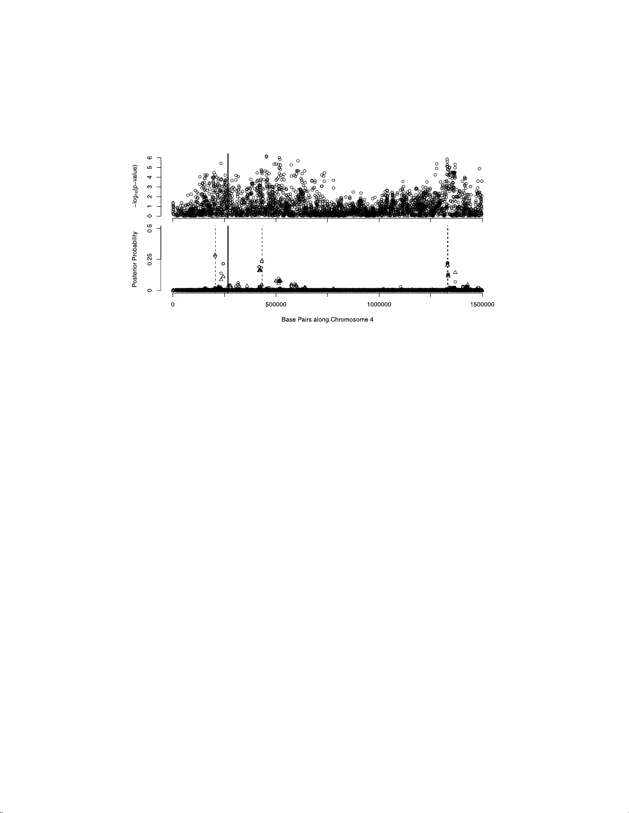
The Annals of Applie d Statistics 2011, V ol. 5, No. 2A, 873–893 DOI: 10.1214 /10-A OAS411 c  Institute of Mathematical Statistics , 2 011 SP ARSE P AR TITIONING: NONLINEAR REGRES SION WITH BINAR Y OR TER TIAR Y PREDICTORS, WITH APPLICA TION TO ASSOCIA TION STUDIES By Doug Spee d 1 and Simon T a v ar ´ e 2 University of Cambridge This pap er presents Sp arse Part itioning , a Bay esian method for identif ying predictors that either individually or in combination with others affect a response v ariable. The metho d is designed for regres- sion problems inv olving binary or tertiary p redictors and allo ws the num b er of predictors to exceed the size of the sample, tw o prop erties whic h make it we ll suited for asso ciation studies. Sp arse Partitioning differs from other regression metho ds by plac- ing no restrictions on how the predictors may influence the resp onse. T o comp ensate for th is generalit y , Sp arse Partitioning implements a nov el wa y of exploring the model space. It searches for h igh p oste- rior probability partitions of th e predictor set, where eac h p artition defines groups of p redictors that join tly influence th e resp onse. The result is a robust metho d that requ ires no prior k now ledge of the t rue predictor–response relationship. T esting on sim u lated data suggests Sp arse Partitioning will typically match the p erformance of an ex isting metho d on a data set whic h ob eys the existing meth od ’s mod el assumptions. When these assumpt ions are viol ated, Sp arse Partitioning will generally offer sup erior p erformance. In tro d uction. In recent y ears association stu dies ha ve sur ged in p opular- it y , driven b y the abilit y to in terrogate the genome in ever-increasing d etail [McCarth y et al. ( 2008 )]. The common aim of these studies is to detect ge- nomic v arian ts th at are link ed with a particular ph en ot yp e. It is hop ed that detecting suc h v arian ts will bring us closer to understanding the biological pro cesses at w ork. Received December 2009; revised Octob er 2010. 1 Supp orted by an EPSRC do ctoral fello wship. 2 Supp orted in part b y NIH ENDGAME Grant U01 HL084706 and NIH Gran t P50 HG02790. Key wor ds and phr ases. Sparse Ba yesian mo deling, nonlinear regress ion, ass ociation studies, large p small n problems. This is an electronic r e print of the or iginal article published by the Institute of Mathematical Statistics in The Annals of Applie d Statistics , 2011, V ol. 5, No. 2 A, 873–89 3 . This reprint differs fr o m the or iginal in pagination and t ypo graphic detail. 1 2 D. SPEED AND S. T A V AR ´ E So far th ese studies ha ve had m ixed r esults. While v ariants with strong effects are pic k ed u p fairly readily [e.g., Th e W ellcome T rus t C ase Control Consortium ( 2007 )], there is sp eculation that more sub tle asso cia tions are b eing missed [Cord ell ( 2009 )]. This suggests the need to dev elop more s o- phisticated tools that are able to explore b ey ond the obvious [Stephens and Balding ( 200 9 )]. F ormally , an asso ciation study can b e view ed as a regression problem consisting of n data p oin ts (the samples) an d N pr edictors (the v arian ts). In th is pap er w e consider the case when eac h p redictor takes either t wo or three unique v alues. T his is common i n asso ciation studies. F or example, a predictor migh t record presence or absen ce of a muta tion, or whether a v arian t is in a neutral, amplified or deleted state. W e also allo w f or “large p , small n problems” in whic h the num b er of predictors exceeds the sample size. Again, this is often the case with asso ciation studies, o w in g to the abund ance of genetic v arian ts a v ailable to examine. Currently a v ailable regression to ols can b e c haracterized b y h ow they p er- mit predictors to influ ence the resp onse. F or example, man y fi t an additiv e mo del, wh ic h o v er lo oks the p ossibilit y th at in teractions b et we en pred ictors migh t affect the resp onse. T he m etho ds whic h p er m it interac tions will gen- erally sp ecify the t yp e of in teractio ns they allo w. A ke y factor affecting p erforman ce is whether the data set b eing examined conforms to the re- strictions the metho d imp oses. Sp arse Partitioning tries to a void placing restrictions on the u nderlying mo del relationship. This sh ould enable it to main tain p o wer in scenarios where other metho ds migh t fail. Section 1 describ es some of the existing metho ds suitable for pr o cessing high-dimensional data. Sections 2 and 3 briefly outline the Sp arse Partition- ing metho dology . S ections 4 and 5 test the p erformance of Sp arse Partition- ing compared to existing m etho ds, wh ile Section 6 concludes the pap er. Ad - ditional details are pro vided in the App end ix and su pplement ary material . 1. Existing metho ds. The task of a regression metho d is to infer how the predictors influ en ce th e resp onse. Let the ve ctor Y (size n × 1) conta in the resp onse v alues and the matrix X (size n × N ) con tain the pred ictors. F or the i th data p oin t, Y i denotes its resp onse, wh ile X i, 1 , . . . , X i,g , . . . , X i,N denote its pr edictor v alues. If we write the regression mo del as l ( E ( Y )) = f ( X ), where l is a sp ecified link function, the aim is to deduce prop erties of f ( X ), the “u n derlying r elationship.” In particular, we wish to identify the subset of predictors that con tribute to ward f ( X ). Consider writing the u nderlying relationship as f ( X ) = f 1 ( X G 1 , 1 , . . . , X G 1 ,s 1 ) + · · · + f K ( X G K, 1 , . . . , X G K,s K ) . Under this representat ion, f ( X ) is infl uenced by additiv e con tributions from groups of in teracting predictors. f k describ es the con trib ution of predictors G k , 1 , . . . , G k ,j , . . . , G k ,s k to f ( X ). In this pap er , add itivit y is not considered SP A RSE P A R TITIONING 3 ONE GROUP MUL TIPLE GR O UPS OF PREDICTORS OF PREDICTORS NO INTERA CTIONS Y = α + β X g e.g., Single Y = α + P N 1 β g X g e.g., SSS INTERA CTIONS Y = f ( X G 1 , . . . , X G s ) e.g., Pairs , CAR T , RF Y = f 1 ( X G 1 , 1 , . . . , X G 1 ,s 1 ) + · · · + f K ( X G K, 1 , . . . , X G K,s K ) e.g., L o gic , M ARS , Sp arse Partitioning Fig. 1. R e gr ession metho ds c an b e c ate gorize d ac c or ding to two fe atur es of their under- lying r elationship. This table shows the four p ossibil ities, for the c ase of binary pr e dictors and a c ontinuous r esp onse. Explanations of the existing metho ds, Single, Pai rs, CAR T, RF, SSS, L o gic and MARS, ar e pr ovide d in the main text. an in teraction. T herefore, the p redictors in eac h group are said to interac t with eac h other, b ut not to interact with a p redictor in a differen t group. F or the most general r elationship, all pred ictors feature in one group. In practice, ho wev er, we su sp ect f ( X ) is far simpler. W e hav e distinguished existing metho ds b ased on tw o features of their underlying relationships: w hether they p ermit more than one group of pr e- dictors to con trib ute to f ( X ) and whether they p ermit in teractions b et ween con tribu ting predictors. Figure 1 demonstrates the four p ossibilities, using the case when the p redictors are binary and the resp onse is con tin u ou s . 1.1. One gr oup, maximum gr oup size one. f ( X ) = f 1 ( X G 1 , 1 ) . The simplest assump tion supp oses the resp onse is influ en ced by only one predictor. Most metho ds in this category are equ iv alent to p erforming a max- im u m lik eliho o d test comparin g a null h y p othesis, f ( X ) = constant , with an alternativ e, f ( X ) = f 1 ( X g ). Single is our imp lemen tation of suc h a metho d. Considering that these metho ds can only detect an asso ciated p redictor b y its marginal effect, they are sur prisingly successful. They are also extremely fast to run and th erefore v ery p op u lar [e.g., Stranger et al. ( 2007 )]. Ba y esian alternativ es are p ossib le [e.g ., Balding ( 2006 )] and u seful if cer- tain pr edictors are though t a priori more likel y to b e asso ciated. Otherwise they will generally pro duce the same results as classical metho ds . 1.2. One gr oup, maximum gr oup size gr e ater than one. f ( X ) = f 1 ( X G 1 , 1 , . . . , X G 1 ,s 1 ) . Ev en for v ery h igh-dimensional problems ( > 500,000 predictors) it is p ossible to test exhaustiv ely all pairwise mo d els [cf. Marchini, Donnelly and Cardon ( 2005 )]. The metho d Pairs is our extension of Single , p er f orming a max- im u m likeli ho o d test for eac h pair of predictors. While the m etho d could b e extended furth er to consider three or four w a y in teractions, this is often infeasible due to computation time. 4 D. SPEED AND S. T A V AR ´ E A second metho d in this category is CA R T [Classification and Regression T rees; Breiman et al. ( 1984 )]. CAR T differs from Pairs in not insisting on the full interact ion mo del for asso cia ted p r edictors. F or example, a CAR T mo del con taining t wo asso ciated p redictors migh t hav e only 3 degrees of free- dom, ev en though there are 4 un ique vecto r v alues p r esen t. Random F orest [Breiman ( 2004 )] offers a sto c hastic in terp retation of this metho d, construct- ing a large num b er of trees in a quasi-random fashion and summarizing their prop erties. 1.3. Mor e than one gr oup, maximum gr oup size one. f ( X ) = f 1 ( X G 1 , 1 ) + · · · + f K ( X G K, 1 ) . This underlying relationship allo ws more than one predictor to b e causal, but restricts the causal pred ictors to con trib uting additive ly . When there are more p redictors th an samp les, the s tand ard multiple regression mo d el will b ecome o ve r-saturated and fail. The classica l solution, adopted by V ariable Subset Selection, Lasso and Ridge Regression [describ ed in Hastie, Tibs h irani and F riedman ( 2001 )], is to introdu ce a p enalt y term that limits the num b er of con trib uting predic- tors. Ho w eve r, this p en alt y term can app ear quite arbitrary . An alternativ e is offered by Ba y esian metho ds [W ang et al. ( 2005 ); Zh ang et al. ( 2005 ); Hoggart et al. ( 2008 )]. These metho ds all o w our preference for sparse m o d- els to b e reflected in the prior distribu tion. W e pic k ed Shotgun Stochastic Searc h [Hans, Dobra and W est ( 2007 )] to represen t this category of m etho ds in the sim ulation studies. 1.4. Mor e than one gr oup, maximum gr oup size gr e ater than one. f ( X ) = f 1 ( X G 1 , 1 , . . . , X G 1 ,s 1 ) + · · · + f K ( X G K, 1 , . . . , X G K,s K ) . Allo wing b oth int eractions and multiple group s of p redictors to con tribu te to the u nderlying relationship has the p otent ial of most accurately describing the tru e mo del. Ho w ev er, b oth decisions in crease the size of the mo del s pace and so the d ifficult y of id entifying the tru e mod el. Logic Regression [Ruczinski, Ko op erb erg and LeBlanc ( 200 3 )] and Mul- tiv ariate Adaptiv e R egression Splin es are t wo of the f ew metho ds in this class. Both metho d s p lace restrictions on the p ermitted fu nctions w h ic h re- duce the size of the mo d el space; L o gic ins ists on Boolean op erators, while MARS uses pro du cts of hinge f u nctions. Sp arse Partitioning falls into this catego ry , b ut places no restriction on the types of functions allo we d. 2. F orm ulating the regression as a partitioning. In order to d escrib e Sp arse Partitioning ’s m etho dology , it is conv enien t to form u late the regres- sion problem as a searc h for h igh s coring partitions. Consider h o w the un- derlying relationship groups predictors: f ( X ) = f 1 ( X G 1 , 1 , . . . , X G 1 ,s 1 ) + · · · + f K ( X G K, 1 , . . . , X G K,s K ) = f 1 ( X G 1 ) + · · · + f K ( X G K ) . SP A RSE P A R TITIONING 5 I = ( G 1 z}|{ 11 G 0 z}|{ 00 G 2 z}|{ 2 ) f ( X ) = f 1 ( X 1 , X 2 ) + f 2 ( X 5 ) ⇒ F or b inary predictors and a contin uous resp onse: Y = α 0 + α 1 , 1 X 1 (1 − X 2 ) + α 1 , 2 (1 − X 1 ) X 2 + α 1 , 3 X 1 X 2 + α 2 , 1 X 5 Fig. 2. An example of a p artitioning for a pr oblem c ontaining five binary pr e dictors (e ach value d 0 or 1) and a c ontinuous r esp onse. The disj oin t s ets G 1 , G 2 , . . . , G K index groups of asso ciated predictors. I f we let G 0 index the “null group”—the group of p r edictors in no w a y associated with the resp onse—then G = { G 0 , G 1 , G 2 , . . . , G K } defin es a partitioning of { 1 , 2 , . . . , N } . In the r epresen tation ab o ve, p redictors are not allo we d to feature in more than one nonn u ll group. T o av oid this restriction, wh ile at th e same time main taining a partitioning, the pr edictor set is expand ed to cont ain C copies of eac h predictor and N is increased accordingly . F or the remainder of this pap er, we describ e the metho d supp osing C = 1, then explain the c hanges required when this is not the case. A partition can also b e describ ed by the vecto r I = ( I 1 , I 2 , . . . , I N ), w here I g indicates to which group predictor g b elongs. This n otation will b e useful later on and also r eminds us that the order in g within groups is not imp or- tan t. Figure 2 giv es an example of a simp le partitioning and the un d erlying relationship to whic h it refers. The fo cus of Sp arse Partitioning is to determine prop erties of the parti- tioning defin ed by the u nderlying r elationship. Ou r main desir e is to iden tify whic h predictors are n ot in the n u ll group. Ho wev er, it is also useful to kno w whether predictors feature in the same nonnull group, indicating in terac- tions. Th e adv antag e of formulat ing the problem in terms of p artitions is that th e mo d el space is lik ely to o v ast to hop e to detect accurately the explicit u nderlying r elationship (i.e., determine f = { f 1 , f 2 , . . . , f K } as we ll as G ). F ortunately , we are us u ally more in terested in detecti ng w h ic h p r e- dictors are inv olv ed, rather than exactly ho w th ey contribute (the latter can b e sa ved for follo w-up analysis). 3. Sparse Parti tioning m etho dology . Sp arse Partitioning is a Ba y esian metho dology , so it follo ws the usual steps of deciding a p rior, calculating th e lik eliho o d , then computing the p osterior d istribution of mo dels through use of Ba y es formula: P (Mo del | Data) ∝ P (Mo d el) × P (Data | Mo d el) . Eac h mo del is defin ed by { G , f } , a p artition and a corresp ond ing set of f u nc- tions. Ho w ever, f is considered a n u isance parameter, so w e are in terested in determining the marginal p osterior P ( G | Data). 6 D. SPEED AND S. T A V AR ´ E 3.1. Prior. P (Mo del) = P ( G , f ) = P ( G ) × P ( f | G ) . The prior for the p artition is based on our b elie f in p g , the pr obabilit y that predictor g is asso ciated with the resp onse. Ther efore, P ( G ) = P ( I ) is constructed s uc h that P I : I g 6 =0 P ( I ) = p g . Two partitions con taining the same asso ciations are giv en equal w eigh t. When m u ltiple copies of eac h predictor are p ermitted, p g equals the probabilit y that at least one copy of pr ed ictor g is asso ciated. Sp arse Partitioning k eeps fi xed the v alues of p g , ho wev er, it is straigh tforward to allo w them to v ary if more detailed prior information is a v ailable. Giv en G k , the relev ant information of fu nction f k can b e describ ed by the v alues it assigns eac h n o de (unique v ector v alue) of X G k . F or th e example in Figure 2 , f ca n b e describ ed b y α = ( α 0 , α 1 , 1 , α 1 , 2 , α 1 , 3 , α 2 , 1 ). Therefore, the prior on f is equiv alen t to a prior on α , for wh ic h Sp arse Partitioning uses a m ultiv ariate normal distribu tion. 3.2. Likeliho o d. The like lih o o d is determined by the regression mo d el. When the r esp onse is conti n u ous (e.g. , a quan titativ e tr ait), Sp arse Parti- tioning supp oses the resid uals are n ormally distr ibuted. When the resp onse is b inary (e.g., a case-con trol exp eriment with affecte d and un affected p a- tien ts), Sp arse Partitioning uses a logit link fun ction. T he marginal lik eli- ho o d is obtained b y integ r ating across the function parameters: P (Data | G ) = Z f P (Data | f , G ) P ( f | G ) d f = Z α P (Data | α , G ) P ( α | G ) d α . 3.3. Posterior. Explicit calculation of P ( G | Data) wo uld require an ex- haustiv e searc h of th e space of partitions, whic h is infeasible eve n for rea- sonably sized problems. Therefore, Sp arse P artitioning uses Marko v Chain Mon te Carlo (MCMC) tec hn iques to estimate statistic s of this p osterior dis- tribution. Within eac h MCMC iteration, tw o samp lin g stages are used: the first prop oses, in tur n, a c h ange to eac h comp onen t of I ; th e second prop oses a c hange to one eleme n t of G . The b ulk of Sp arse Partitioning ’s pr o cessing time is sp ent sampling from the p osterior distribution. T herefore, it is con ve- nien t that the t w o stage s can b e p arallelized with an almost linear sp eed-up. F ull details of the metho dology are pr o vided in App end ix and Sections 1, 2 and 3 of the Su pplementa r y Material [Sp eed and T av ar´ e ( 2010 )]. 4. Sim u lation studies. In total, ten sim u lation studies w ere carried out, designed to test v arious asp ects of Sp arse Partitioning ’s p erformance and mak e comparisons with existing metho ds. This section pr esen ts resu lts from the fi r st study . F ur th er details of the metho ds used to simula te data and SP A RSE P A R TITIONING 7 T able 1 The first simulation study c onsider e d thr e e differ ent under lying r elationships Mod el Underlying relationship I Y = X 1 + 1 . 5 X 2 − 2 X 3 I I Y = 1 . 5 X 1 × X 2 + X 3 I I I Y = f ( X 1 , X 2 ) + X 3 ; f (0 , 0) = 0, f (1 , 0) = 1, f (0 , 1) = 2, f (1 , 1) = − 1 the results from the remaining n in e studies are pro vid ed in Section 4 of the Supp lemen tary Material [Sp eed and T a v ar ´ e ( 2010 )]. T yp ically , eac h sim ulated data set consisted of 100 s amp les, eac h of 1000 predictors, thr ee of w hic h w ere causal for the resp onse. Eac h regression metho d wa s ask ed to iden tify its top th ree associations and w as then scored b y ho w man y causal predictors it correctly iden tified. Emp irical estimates w ere obtained by av eraging o v er 100 data sets. The fir st study examined the case of (uncorr elated) binary pred ictors and a con tinuous resp onse. Eac h scenario concen trated on a particular underly- ing relationship (Mod els I, I I or I I I) for a particular frequency of the causal predictors (0.05, 0.1, 0.2, 0.4 or random). Th e first mo d el w as designed so that eac h causal predictor contributed additiv ely , the second featured a multiplica tiv e in teractio n, while the third in volv ed a “w eird” in teraction (see T able 1 ). Figure 3 presents results from the first stu dy . Eac h plot relate s to a differ- en t underlying relationship. Within eac h p lot, th e lines display the a v erage n u m b er of causal pr edictors correctly iden tified by eac h metho d for different frequencies of the causal p redictors. Figure 4 provi des an alternativ e in- terpretation of th ese results, r ep orting h o w often eac h metho d successfully detected 0, 1, 2 or 3 causal predictors for eac h scenario. Fig. 3. Each plot c onsiders a differ ent underlying r elationship (descr ib e d in the main text). Within e ach plot, the lines r ep ort the aver age numb er of c ausal pr e dictors c orr e ctly dete cte d by e ach metho d for differ ent c ausal pr e dictor fr e quencies (“?” denotes r andom). 8 D. SPEED AND S. T A V AR ´ E Fig. 4. Each gr oup of ei ght vertic al b ars c omp ar es the metho ds for a p articular underlying r elationship and c ausal pr e dictor fr e quency (“?” denot es r andom). Within e ach b ar, the lengths of the shade d se ctions (fr om top to b ottom) indic ate the pr op ortion of time the metho d c orr e ctly dete cte d 0, 1, 2 and 3 c ausal pr e dictors. F or example, the l engths of the darkest gr ay b ars show how often e ach metho d suc c essful ly identifie d al l thr e e c ausal pr e dictors. F or al l sc enarios, the or dering of metho ds is the same (fr om left to right): Single, P airs, CAR T, R F, SS S, Logic, MARS and Sparse P artitioning . Under Mod el I, SSS , L o gi c , MARS and Sp arse Partitioning were the four b est p erforming metho d s across differen t frequencies, p ulling clear of Single , Pairs an d RF as the causal pr edictor f requency increased. Und er Mo d el I I, this order w as essen tially main tained, with the exception of SSS , whic h dropp ed into the second tier of p erform er s . Ho wev er, un der Mo d el I I I, Sp arse Partitioning h as emerged on top, comprehensively b eating six of its riv als, with only Pairs coming close. Sp arse Partitioning h as p erformed b est in this sim u lation study , pro ving itself most robu s t across the differen t mo dels. It has triump hed un d er Mo- del II I, when th e underlying r elationship assump tions of all other metho ds ha ve b een violate d. Note that its generalit y h as not prev en ted it fr om at least matc hing the p erformance of th e existing metho d s u nder Mod els I and II . 5. Application to real d ata sets. W e applied Sp arse Partitioning to four previously analyzed association stud ies: the first looked at expression data for 109 ind ividuals in the HapMap pro ject ( h ttp://hapmap.n cbi.nlm.nih.go v ); the s econd an d third examined data sets from the “2010 Pro ject” ( h ttp:// w alnut.usc.edu/2010 ), a large-scale study of the plan t Ar abidops is tha liana ; the fourth used data p r o vided by the Flin t lab oratory at the Univ er s it y of Oxford ( h ttp://www.well.o x.ac.uk/flin t-2 ). Extended v ersions of all results are pro vided in Figures 12–16 of th e Su pplementa ry Material [Sp eed and T a v ar ´ e ( 2010 )]. 5.1. HapMap data. Dr. Antigo n e Dimas kindly p ro vided us with a sam- ple of 109 individuals, eac h t y p ed for 1,186 ,075 Sin gle Nucleot ide Po lymor- phisms (S NPs) and measured for expression lev els of 2682 genes [Dimas ( 2009 )]. W e applied Sp arse Partitioning to the four genes for whic h Dr. Di- mas foun d strongest evidence f or an in teraction, cop yin g her decision to SP A RSE P A R TITIONING 9 Fig. 5. Analysis of expr ession levels of MTHFR using HapMap data. The top plot shows r esults fr om Single , the b ottom plot shows r esults fr om two runs of S parse Partitioning . F ul l details ar e pr ovide d in the main text. consider only SNPs within one million base pairs (1 Mbp) of eac h gene. Figure 5 presents the results f or MTHFR , the third of these genes, lo cated appro ximately 11. 8 Mbp along C hromosome 1. F or eac h SNP in th e 2 Mbp region, the top plot d ispla ys the p -v alue ob tained by Single , while the b ottom plot rep orts th e p osterior probabilit y of asso ciation from Sp arse Partitioning (circles corresp ond to run one resu lt, triangles to run t wo). The solid ve rtical line marks the lo cation of the gene, while the t w o dashed v ertical lines mark the lo cations of the SNPs declared in teracting by Dr. Dimas. The dashed horizon tal lines p ro vid e estimates of the 5, 25 and 50% signifi cance thresholds for the top association of eac h method , calc u lated using p ermutation tests. Sp arse Partitioning f ou n d three promisin g SNPs, rs2286139 , rs26438 88 and rs2279703, with p osterior p r obabilities of asso ciation 0.57, 0.96 and 0.96, resp ectiv ely . It is no coincidence that the second and th ird hits ha ve matc h- ing pr obabilities. Before analysis, Sp arse Partitioning searc hes for h ighly correlated pr ed ictors, as is often the case with fine-scale genetic data. SNP rs264388 8 was foun d to b e highly correlated w ith SNP rs2279703, with matc hing v alues for 106 of the 109 individ uals. Therefore, the former SNP w as remo ved from analysis, and su bsequentl y giv en the same p osterior es- timates as th e latter. Sp arse P artitioning returned a p osterior probabilit y of in teraction of 0.42 b et we en SNPs rs2286139 and rs264388 8/rs2279 703 (indicated b y the h orizon tal arrows), offering some supp ort for Dr. Dimas’ findings of an in teraction. 5.2. 2010 pr oje c t: Pilot data. The pro ject’s pilot data set lo oke d at 95 accessions, genot y p ed for 5419 SNPs and measured for ten phen ot ypic traits. W e fo cused on the ten th p henot yp e, expression lev els of the FRIG IDA gene. 10 D. SPEED AND S. T A V AR ´ E Fig. 6. Analysis of expr ession levels of FRIGIDA for A r abidopsis thaliana. The top plot shows r esults fr om Single , the b ottom plot shows r esults fr om two runs of Sp arse Parti- tioning . F ul l details ar e pr ovi de d in the main text. W e decided to r emo ve eigh t acce ssions whose genot yp es w ere either almost iden tical to remaining accessions or w ere fl agged as suspicious b y principal comp onent analysis. Using metho d s similar to the original analysis [Zhao et al. ( 2007 )], we firs t adju sted the p henot yp e to correct for confound ing due to p opulation structure and relatedness of ac cessions. By con trast, w e c hose not to impu te missing v alues, m eanin g appro ximately 10% of the genot yp es w ere su pplied to Sp arse Partitioning as u nobserve d. Figure 6 compares the p -v alues obtained from Single to the p osterior probabilities of asso ciation of Sp arse Par titioning . Our metho d identified just one strong asso ciation, coinciding with the thir d strongest hit of Single and su ggesting that, in this case, the simp le under lyin g relationship of Single migh t b e appropriate. F or b oth metho d s the strong asso ciations la y v er y close to the FRIGIDA region, marked b y a solid v er tical line, suggesting the results are accurate. A p ossible concern is that Sp arse P artitioning ’s generalit y migh t lead to o verfitting on o cca s ions wh en simple mo d els are more app ropriate. Here that do es n ot app ear to b e the case, with Sp arse Partitioning declaring only one strong asso ciation. W e r ep eated the an alysis usin g imputed data, whic h allo w ed us to compare the pr ediction accuracy of eac h method via lea ve-o ne- out cross-v alidation. The linear mo del con taining only the top h it from Single explained 44% of the v ariance, agreeing closely with Sp arse Partitioning ’s estimate of 42% v ariance explained. 5.3. 2010 pr oje c t: R ele ase 3.04. W e examined ho w Sp arse Partitioning w ould deal with a problem encount ered in the 2010 pr o ject’s m ost recen t pap er [At w ell et al. ( 2010 )]. Th e expression level of the F LC gene is kno wn to SP A RSE P A R TITIONING 11 Fig. 7. A nal ysis of expr ession l evels of FLC for Ar abidopsis thaliana. The top pl ot shows r esults fr om Single , the b ottom plot, which has a trunc ate d y -axis, shows r esults fr om two runs of Sparse Partitioning . F ul l details ar e pr ovide d i n the main text. b e affected by p olymorphisms in the FR IGIDA region [Johans on et al. ( 2000 ); Shindo et al. ( 2005 )]. At w ell et al. p erformed a one-SNP-at-a-time asso cia- tion study using F LC expression as the r esp onse. Its analysis pro d uced resu lts similar to ou r analysis by Single , sho w n in the top plot of Figure 7 . Wh ile some S NPs within the F RIGIDA region (whic h is marked by a ve rtical line) ac hiev ed genome-wide significance, tw o stronger groups of asso ciations were detected app ro ximately 200 kb p and 1 Mbp to the right. Prior kn o wledge w ould suggest th ese do wnstream associations are spurious. When A t well et al. rep eat ed the an alysis, b ut this time in cluding in the r egression m o del t wo alleles of the FRIG IDA gene kno wn to affect FLC , the d o wns tream asso ci- ations v anished, increasing suspicion that they were false p ositiv es. F or th e rest of this section, we assume th is to b e the case. The pr o ject’s latest d ata release pro vides t yping for 214,553 SNPs across fiv e c hromosomes. W e pick ed the 3509 SNPs lo cated within th e fi r st 1.5 Mb p of Chromosome 4. As this subset w as a biased selecti on (e.g., it con tained o ve r t wo- thirds of those SNPs w ith marginal p -v alues less than 10 − 4 ), it w as necessary to reflect this when c h o osing the prior probabilit y of association for Sp arse Partitioning . In the even t, we settled up on a prior probability of 1 in 350 0. W e used imp uted data for this analysis, as the in creased SNP dens ity allo w ed missing v alues to b e inferr ed more r eliably . Similar to th e analysis of At w ell et al., we decided to correct only for relatedness, as d iscussions with memb ers of the Nordb org group con vin ced us that adjusting for p op- ulation structure risked removing to o m uch true signal. T he b otto m plot of Figure 7 sho ws the results of Sp arse Partitioning . The dashed v ertical lines 12 D. SPEED AND S. T A V AR ´ E indicate th e three regions where our method found most evidence of associ- ation. While t wo false p ositiv es r emained, Sp arse Partitioning gav e greatest recognition to the FRIGIDA region, id en tifying a p ossib le association appro x- imately 60 kbp upstream of th e gene. In this example, w e had kno wledge of the true causal region, allo wing us to id en tify the false asso ciations. The concern is that this example is one of man y , and that most times w e will not kno w the correct answ er. In these cases, th e b est we can hop e is that a m etho d ac knowledge s the tru e and false p ositiv es, but r ecognizes the u ncertain ty . Th is is w h at Sp arse Partitioning has done h ere. F urtherm ore, our metho d more pr ecisely identified p eaks th an Single whic h should sp eed up the v er ifi cation pro cess. 5.4. Mouse data. Jon Krohn, fr om P rofessor Jonathan Flin t’s group at the Unive r sit y of Oxford, kin d ly pro vided us with C D4 coun ts for 1274 “het- erogeneous stock” mice [Solb erg et al. ( 2006 )], along with genot ypic v alues for 770 S NPs co vering the length of Chromosome 5. Kr ohn h ad pr eviously analyzed this data set using Bagphenotyp e , soft wa r e d esigned b y Dr. William V aldar ( http://w ww.unc.e du/ ~ wvaldar/ bagpheno type.htm l ). The resp on- se v alues were con tinuous, while the predictors were tertiary . On ly a tiny prop ortion of genot y p es (0.1%) were missing, so we sa w no need to imp ute v alues and instead left them as u nobserved. In addition, we we re pro vided with the gender of eac h mouse, w h ic h w e co ded as a binary v ariable and included in the set of p redictors. As the c hromosomal region w as a su bsection of a genome-wide study , w e decided a prior probability of asso ciation of 1 in 10,000 w as appropri- ate for eac h SNP . There is o v erw helming pr ior kno w ledge that C D4 coun ts are link ed to gender [e.g ., Maini et al. ( 1996 )], so we decided up on a prior probabilit y of 0.5. W e run Sp arse Partitioning allo wing thr ee copies of eac h predictor ( C = 3). As Figure 8 demonstrates, the top hits from Single , SNPs CEL-5 10658 4673 and rs13478460, whic h d ue to link age disequilibrium are almost iden tical, p ersisted in Sp arse Partitioning . In add ition, our metho d declares asso ciat ed SNP rs1347815 6. As in d icated by the h orizon tal arro ws , Sp arse Partitioning found evidence of interact ions b et ween gender and the top SNPs. T o test the effect of our pr ior choi ces, we rep eated the analy- sis w ith p rior p robabilities { 10 − 4 , 0.1 } , { 10 − 3 , 0.5 } and { 10 − 3 , 0.1 } , and obtained v ery sim ilar r esults on eac h o ccasion (results not sho w n). Maxim um lik eliho o d tests offer justification f or w h y rs134781 56 wa s found b y Sp arse Partitioning , b ut largely o ve rlo ok ed by Single . Th e supp lemen tary material pro vides plots for t w o sets of tests. T h e first set compares, for eac h SNP , the pairwise in teraction with gender agai nst a n ull mo d el of no asso ciation. W e find that the top hits of Single remain the most significan t hits here. Ho wev er, these tests provi de only limited in formation ab out the strength of the inte r action terms. Th erefore, the second set compares th e SP A RSE P A R TITIONING 13 Fig. 8. Analysis of CD4 c ount in m ic e. The top plot shows r esults fr om Single , the b ottom plot shows r esults fr om two runs of Sp arse Pa rtitioning . F ul l details ar e pr ovide d in the main text. pairwise interact ion mo del aga inst the additiv e m o del for that SNP and gender. W e see that the int eraction b et w een rs13478156 and gender is highly significan t. Th is su pp orts Sp arse Partitioning ’s claim that th is SNP ac ts in a gender sp ecific wa y , whic h also agree s with find ings from Krohn’s analysis. This data set demonstrated the adv an tage of allo wing multiple copies of eac h predictor. When Sp arse Partitioning is ru n without this option (results for C = 1 are sho wn in the sup plemen tary material), the b est fitting partition features three asso ciated predictors in a single nonnull group . The p osterio r estimates of pairwise int eractions cannot b e tru sted b ecause the metho d is unable to distinguish b et wee n, sa y , a single three-wa y in teraction and a pair of t wo -wa y in teractions. Allo w ing m ultiple copies of p redictors requires only a small increase in compu tation time, so w e recommend this option is us ed . 6. Discussion. It is fairly easy to design a regression metho d that is finely tuned for a sp ecific u nderlying relationship and then demonstrate its sup erior p o wer on d ata sets whic h ob ey this mo d el. If one were presented only with the results of the Model I I I sim ulations, it would b e easy to think that Sp arse Partitioning is suc h a metho d. W e ha ve tried to sh o w this is not case. W e b eliev e th at Sp arse Partitioning offers a robust alternativ e to existing metho ds. It fares equ ally w ell u nder sim p le mo d els, bu t comes in to its o wn as the mo del b ecomes more complex. 6.1. Pr osp e cts for nonline ar r e gr ession. Nonlinear regression metho d s are comp eting o ve r a fairly small share of the mark et, b ounded on the one s id e by the p erformance of metho ds s u c h as Single and on the other b y the strength 14 D. SPEED AND S. T A V AR ´ E of signal present in the data. Despite these limitati ons, th ere remains a de- mand for suc h metho ds . There are many examples wh ere standard linear metho ds fail to explain a satisfactory p ercent of the v ariation, so it is quite p ossible th at n onadditiv e systems are at w ork. Sp arse Partitioning should not b e view ed as a s earch for in teractions, but rather as a r egression metho d whic h b ears in teractio ns in mind. Even for situations in w hic h it cannot pinp oin t an in teraction with certain ty , its detect ion p ow er should b enefit for ha ving considered their existence. 6.2. Gener ality. Sp arse P artitioning ’s strength deriv es fr om the gener- alit y of its und er lyin g r elationship. Therefore, it is p erhaps a surprise th at the metho d do es not app ear to suffer in situations w here this r elationship is o v erly complicated. The r esults in Section 4 su ggest th ere is no in h eren t disadv an tage to using suc h a general un d erlying relationship. While Sp arse Partitioning will almost certainly o v erfit the true mod el at some p oin ts in the MCMC s amp ling, its p osterior estimates are b ased on mo del a v er ages, rather th an the single h ighest scoring mo del v isited. F or this reason, it should not m atter if a nonasso ciated predictor is occasionally declared asso ciated, as these errors are like ly to b e spread thinly across the noncausal predic- tors. Additionally , as Sp arse Partitioning seeks only to estimate marginal p osterior probabilities, us in g an underlying relationship to o general should not upset the Ba y esian mec h anics. The p rior probabilit y that a predictor is asso ciated remains constan t (equal to p g ) regardless of the size of the mo del space. Ev en if excessive generalit y do es affect some asp ects of the p osterior distribution, the marginal p osterior probabilities should remain correct. 6.3. Diagnosis. The only wa y to calculate the p osterior d istribution ex- actly is through an exhaustive searc h of th e sp ace of partitions. Unfortu- nately , this is feasible for only the smallest data sets, so instead Sp arse Par- titioning is forced to explore the mo d el sp ace in a step wise fashion. In this resp ect, Sp arse Partitioning ’s searc h holds an adv an tage o v er deterministic algorithms. When deciding which mo del in th e neigh b orhoo d to visit n ext, Sp arse Partitioning is n ot forced to mov e to th e highest scoring mo del. In- stead it is able to try a lo wer scoring m o ve , in the hop e that this is a gatew a y to a higher scoring r egion. The drawbac k of this sto chastic it y is the v ariabilit y it in tro d uces in to Sp arse P artitioning ’s results. Th e analysis in Section 5 pro vides some tips for gauging Sp arse Partitioning ’s p erformance. It is sensible to compare the results with those of Single , as w e w ould exp ect v er y strong asso ciations to b e foun d by b oth metho ds. Rep eating the analysis w ith a n ew random seed will highligh t ob vious lac k of con v ergence, as should examination of trace plots. Add itionally , if time p ermits, rep eati ng the analysis with th e resp onse v alues p erm u ted will p ro vid e significance thresh olds u nder a mo d el of no true associations. SP A RSE P A R TITIONING 15 6.4. Limitations. The p ro cessing time required for eac h iteration s cales linearly with N . W e sp eculate that the n u m b er of iterations required for con verge n ce scales approxima tely with th e 1.5th p o wer of N (based on the step wise nature of Sp arse Partitioning ’s searc h) and exp onen tially with the n u m b er of true associations (based on the gro wth of the mo del space). As a rule of thum b, w e consider Sp arse Partitioning su itable for problems with no more than 20,000 predictors, or cases where N /n < 100. T his is not to sa y that Sp arse Partitioning cannot b e applied on, sa y , a genome- wide s cale, but it ma y b e necessary to filter th e pr edictors fir st. W e suggest pic king, f or example, the h ighest 10% of hits fr om Single . Of course, th is is not ideal. It is certainly p ossible that true asso ciations are concea led within the remainin g 90% of predictors. But considerin g standard practice in volv es pic king, p er h aps, the top 10 0 hits of Single for fur ther analysis, the abilit y to consider instead the top few thousan d hits should offer a significan t adv an tage. As w e exp erienced in Sectio n 5 , it is imp ortan t to realize when w e ha ve selected a biased sub s et of predictors and reflect this in the pr ior probabilit y of asso ciation. Th e easiest solution is to p ic k the p riors as if analyzing the complete set of predictors. W e ha v e id en tified situations in whic h Sp arse Partitioning will struggle. Examples w ere found in Simulatio n Stu d ies Fiv e and T en (see S upplemen- tary Mat erial). The latter was an almost una v oidable situation b ecause the true relationship h ea vily con tradicted our p rior b eliefs. The former demon- strated the drawbac k of treating tertiary p redictors as catego rical v ariables, when in fact their v alues h a ve a natural order in g. W e susp ect th at this problem can b e o ve rcome b y application of a Ba yesia n version of P ro jection Pursuit [describ ed in Hastie, Tibshirani and F riedman ( 2001 )] that we are no w d ev eloping. Additionally , consider the case in whic h the resp ons e is influenced b y an int eraction of t w o predictors, b u t the inclusion of neither p redictor on its o wn significan tly impr ov es the mo del fit. F or one of these predictors to ha ve a realistic chance of b eing included in a n onn ull group, th e impr o ve- men t in fit must offset the p enalt y of inclusion imp lied b y P ( G ). Because of the sin gle-step nature of Sp arse Partitioning ’s search, it is unlik ely that either p redictor will app ear in the current mod el, wh ic h is required f or the metho d to consider their interact ion. F or our metho d to b e su ccessful in this case, it w ould hav e to p er m it tw o-step m o ve s or resort to an exhaustive searc h. Sp arse Partitioning can b e used when the predictors are con tinuous, pro- vided a suitable transformation exists. F or example, we h av e applied our metho d to cop y n um b er v alues, b y first reducing eac h co n tinuous mea- surement to one of three classes (neutral, increased or decreased). In the same w a y , we hop e our metho d can b e applied to a whole range of prob- lems. 16 D. SPEED AND S. T A V AR ´ E APPENDIX: DET AILS OF BA YES IAN FRAMEW ORK The regression mo del is written as l ( E ( Y )) = f ( X ), where l is a sp eci - fied link function and f ( X ) is the “u n derlying relationship.” Without loss of generalit y , the und erlying r elationship can b e exp ressed as the sum of functions of groups of associated pr ed ictors: f ( X ) = f 1 ( X G 1 ) + f 2 ( X G 2 ) + · · · + f K ( X G K ) . The disjoint sets G 1 , G 2 , . . . , G K index groups of asso ciated predictors. Let G 0 , the “null group,” ind ex the p redictors n ot asso ciated. Therefore, G = { G 0 , G 1 , G 2 , . . . , G K } partitions { 1 , 2 , . . . , N } . Equ iv alent ly , the parti- tion can b e describ ed by the vecto r I = ( I 1 , I 2 , . . . , I N ), where I g indicates to whic h group the g th predictor b elongs. Only un iqu e partitions are con- sidered, so the ordering of elemen ts within group s is irrelev an t, as is the ordering of nonn ull groups. A sin gle mo del will b e { G , f } , a partition and a corresp onding set of func- tions { f 1 , f 2 , . . . , f K } . The mo del space will b e all suc h p ermissible pairs. If w e wish to allo w predictors to f eature in more than one group of asso cia- tions, the pr edictor set is expand ed to con tain C copies of eac h predictor. An alternativ e approac h is to ke ep one copy of eac h predictor, but r elax the con- dition on d isjoin t groups. Ho we ver, we felt this appr oac h created a great er amoun t of duplication within the space of underlying r elationships, making it more c hallenging to defi ne a prior. T he description of the metho d sup p oses C = 1, with the alternativ e case discussed when n ecessary . W e are in terested in the p osterior distribution of G and f , giv en the observ ed v alues for X and Y . T o b e fully Ba y esian, w e must also consider the distr ibution of the predictors, wh ic h can b e w r itten as P ( X | ε ), f or some parameter v ector ε : P ( G , f , ε | X , Y ) ∝ P ( G , f , | X , Y ) × P ( ε | G , f , X , Y ) . If w e assume ε is un affected b y G and f [Gelman et al. ( 2004 )], its p osterior can b e ignored in the calculation of P ( G , f | X , Y ) . Similarly , as we only wish to estimate p rop erties of the p oste rior d istribution of partitions, w e treat the functions as n uisance parameters: P ( G | X , Y ) ∝ P ( G | X ) × P ( Y | X , G ) = P ( G | X ) × Z f P ( Y | f , X , G ) P ( f | X , G ) d f , with P ( G | X ) reducing to P ( G ) , as we su pp ose the p r ior distribution of G do es not dep end on the obser ved v alues of the predictors. A.1. P artition p rior, P ( G ) . Th e p rior for th e partition is constructed so the prob ab ility that pred ictor g is asso ciated equ als p g . F or partition I , we can define the equiv alence class [ I ] con taining all partitions that declare SP A RSE P A R TITIONING 17 the same predictors asso ciated. T o ensure the marginal p robabilit y that predictor g is asso ciated equals p g , w e desire P ([ I ]) = X I ′ ∈ [ I ] P ( I ′ ) = Y j : I j =0 (1 − p j ) Y j : I j 6 =0 p j = Y j ∈ G 0 (1 − p j ) Y j / ∈ G 0 p j , b ecause then P ( I g 6 = 0) = X I : I g 6 =0 P ( I ) = X [ I ]: I g 6 =0  Y j : I j =0 (1 − p j ) Y j : I j 6 =0 p j  = p g Y j 6 = g [(1 − p j ) + p j ] , equaling p g , as required. Assigning equal w eigh ting to mem b ers of [ I ] , we can calculate P ( I ) explic- itly b y counting the s ize of eac h equiv alence class. If I d eclares s = N − | G 0 | predictors asso ciated, then th e size of [ I ] will b e the num b er of wa ys s ele- men ts can b e partitioned. Unrestricted, this w ould equal the s th Bell n u m- b er. I nstead, Sp arse Partitioning limits eac h partition to n o more than K nonnull groups, eac h con taining at most S elemen ts. These “trun cated” Bell n u m b ers, B ( s, K , S ), can b e calculated in a recursiv e fashion. Let a j denote the n u m b er of group s of size j f or j = 1 , 2 , . . . , S . Then B ( s, K , S | a 1 , a 2 , . . . , a S − 1 , a S ) = B ( s, K , S | a 1 − 1 , a 2 , . . . , a S − 1 , a S ) + B ( s, K , S | a 1 + 1 , a 2 − 1 , . . . , a S − 1 , a S )( a 1 + 1) + · · · + B ( s, K, S | a 1 , a 2 , . . . , a S − 1 + 1 , a S − 1)( a S − 1 + 1) , with b ound ary condition B (0 , K, S | a 1 , a 2 , . . . , a S − 1 , a S ) =  1 , if a j = 0 ∀ j , 0 , otherwise. Equally w eighting eac h member of [ I ] places a high pr obabilit y (1 − | [ I ] | − 1 ) on the existence of inte ractions, ev en though few interac tions hav e so far b een found and v er ifi ed. It wo u ld b e straight forw ard to alter the partition w eightings. F or example, w e could c ho ose to fav or partitions con taining fewer in teractions. How ev er, th e lac k of kno wn in teractions must largely b e du e to ho w hard they are to identify , coupled with h o w rarely they are s earc hed for. Therefore, w e are satisfied that a u n iform w eigh ting is a reasonable c h oice. Sp arse Partitioning requires that K and S are set in adv ance, to al- lo w su fficien t memory to b e allocated and pre-calculation of B ( s, K , S ) . Theoretically , K and S should b e no smaller than N , to ensur e the tw o most extreme u nderlying relatio nships are p ossible (either N groups of size 18 D. SPEED AND S. T A V AR ´ E one or one group of size N ). In practice, these v alues would require v ast amoun ts of unn ecessary computation. Th erefore, we suggest K and S are set to the smallest v alues p ossib le, without impacting th e direction of the MCMC c hain. The calculation of P ( I g 6 = 0) assumes K × S ≥ N , as the last summation supp oses all 2 N equiv alence classes are ac hiev able. When this condition do es not hold, th e error inv olv ed can b e calculated f or the case that all prior probabilities are equal: P ( I g 6 = 0) = p g K S − 1 X s =0  N − 1 s  p s g (1 − p g ) N − 1 − s  K S X s =0  N s  p s g (1 − p g ) N − s = p g P ( s ≤ K S − 1 | s ∼ B ( p g , N − 1)) / P ( s ≤ K S | s ∼ B ( p g , N )) . Using a n ormal appro ximation for eac h b inomially distributed v ariable, w e obtain P ( I g 6 = 0) = p g Φ  K S − 1 / 2 − ( N − 1) p g p p g (1 − p g )( N − 1)  Φ  K S + 1 / 2 − N p g p p g (1 − p g ) N  , where Φ is the cum u lativ e probab ility function for a standard normal. F or small p g , the v alue of P ( I g 6 = 0) is affected most by the pr ior mean, N p g . W e suggest setting K = 4 and S = 4. Entering these v alues into the equation ab o ve, we fin d that th e actual pr ior probability of asso ciation us ed by Sp arse Partitioning lies within 1% of the desired v alue, p g , ev en when the pr ior mean is as high as 9. When m ultiple copies of predictors are allo we d ( C > 1), the p rior proba- bilit y of association for eac h cop y of pr edictor g is set to 1 − C p (1 − p g ). Th is ensures the pr obabilit y that one or more copies of pred ictor g are asso ciated remains equal to p g . Allo wing multiple copies of predictors creates an ele- men t of duplication within the space of partitions. F or example, a partition in w hic h t wo copies of a pr edictor feature in the same nonnull group ef- fects the same underlying relationship as the partition obtained when one of these copies is remo v ed. As a result, the p rior w eigh ting for this underlyin g relationship is increased. Ho w ever, for small v alues of p g this effect will b e negligible. As with K and S , it is necessary to sp ecify C in adv ance. Its v alue has m inimal effect on compu tation time, so we recommend a conserv ativ e setting, suc h as C = 3 . A.2. F u nction p rior, P (f | G ) . T o ensure identifiabilit y of the fun ctions, one v alue of X G k is considered the base v alue and its mappin g is absorb ed in to the o v erall in tercept (d en oted b y α 0 ). Therefore, f k has degree of free- dom one less than d k , the num b er of uniqu e v alues (no d es) of X G k . Let SP A RSE P A R TITIONING 19 V k , 1 , V k , 2 , . . . , V k ,d k − 1 b e dummy bin ary v ariables that d istinguish the re- maining d k − 1 no d es; these map to α k , 1 , α k , 2 , . . . , α k ,d k − 1 , resp ectiv ely . The underlying relationship can b e written in standard regression form: f ( X ) = α 0 + ( α 1 , 1 V 1 , 1 + · · · + α 1 ,d 1 − 1 V 1 ,d 1 − 1 ) + · · · + ( α K, 1 V K, 1 + · · · + α K,d K − 1 V K,d K − 1 ) . All the relev an t information of the functions is con tained in the v ector α = { α 0 , α 1 , 1 , . . . , α 1 ,d 1 − 1 , . . . , α K, 1 , . . . , α K,d K − 1 } , of size D = 1 + P ( d k − 1). Sp arse Partitioning assigns indep enden t n ormal priors with mean 0 to eac h elemen t of α . These can b e viewe d as a p enalt y on smo othn ess, b ut one whic h accepts that with categorical predictors there is n o orderin g to the no des. This agrees with a b elief in p arsimon y , whic h pr efers simple functions to complicat ed ones. In the con tinuous resp onse case the v ariance of th ese n ormal priors is σ 2 /r ; in the b inary resp onse case the v ariance is 1 /r . In b oth cases, the c hoice of r con trols th e exten t by whic h smo othness is app lied. Typicall y we set r to 1. A.3. Lik eliho od, P (Y | f , X , G ) . When the resp onse is cont in u ous, the link function is the identit y and the residuals are assumed to b e in dep end en t dra w s from a normal distr ibution with mean zero and v ariance σ 2 : P ( Y | f , X , G ) = Z σ 2 P ( Y | σ 2 , f , X , G ) P ( σ 2 ) dσ 2 = Z σ 2 (2 π σ 2 ) − n/ 2 exp  − 1 2 σ 2 ( Y − f ( X )) T ( Y − f ( X ))  σ − 2 dσ 2 . This integ ral in corp orates a prior for σ 2 of the form σ − 2 , wh ich reflects a p reference f or smaller v ariances. It do es not matter that this prior is im- prop er as it is co mmon to all mo d els. When the r esp onse is binary , a logit link fun ction is used, l ( a ) = log ( a 1 − a ): P ( Y | f , X , G ) = Y i [ l − 1 f ( X i. )] Y i [1 − l − 1 f ( X i. )] (1 − Y i ) . A.4. Marginal lik eliho o d, P (Y | X , G ) . P ( Y | X , G ) = Z f P ( Y | f , X , G ) P ( f | X , G ) d f = Z α P ( Y | α , X , G ) P ( α | X , G ) d α . With a cont in u ous resp onse, P ( Y | X , G ) can b e calculated explicitly . When the resp onse is binary , Sp arse Partitioning uses a Laplace appro ximation. 20 D. SPEED AND S. T A V AR ´ E Let W ( α ) = P ( Y | α , X , G ) P ( α | X , G ) and w ( α ) = log( W ( α )): w ( α ) ≈ w ( α ′ ) + ( α − α ′ ) T dw ( α ′ ) d α + 1 2 ( α − α ′ ) T d 2 w ( α ′ ) d α 2 ( α − α ′ ) . If ˆ α is the maxim um like liho o d estimate of w ( α ) , then W ( α ) ≈ W ( ˆ α ) exp  − 1 2 ( α − ˆ α ) T  − d 2 w ( ˆ α ) d α 2  ( α − ˆ α )  . Therefore, P ( Y | X , G ) ≈ P ( Y | ˆ α , X , G ) P ( ˆ α | X , G )(2 π ) D / 2     − d 2 w ( ˆ α ) d α 2     − 1 / 2 . Alternativ ely , Sp arse Partitioning allo w s the user to select a pr obit link function, in wh ic h case a late n t v ariable repr esen tation of the like liho o d can b e used [Alb ert and Chib ( 1993 )]. Essential ly , eac h b inary resp onse is replaced by a conti n u ous “pseud o resp onse.” The regression mo d el is then treated as if it w er e linear, except the new resp onse v alues are resampled once p er iteration. When there are tw o or more fu nctions present , the marginal likelihoo d will b e affected (ve ry sligh tly) by whic h n o de is considered the base v alue for eac h function. F or consistency , the n o de remo v ed is c hosen acco rding to a defined rule (and is the zero vec tor of X G k if av ailable). In add ition, b efore analysis b egins, con tin uous resp onse v alues are transformed to ha ve mean 0 and v ariance 1 to redu ce v ariabilit y caused b y the c hoice of base v alue. Soft ware. Sp arse Partitioning has b een implemen ted and is a v ailable at http://w ww.compb io.group .cam.ac.uk/software.html . Ac kn o wledgment s. The auth ors thank An tigone Dimas, Keyan Zhao, Bjarni Vilhj´ almsson an d Jon Krohn for pr o viding data from their resp ectiv e lab oratories. W e thank Alexandr a Jauh iainen, T err y Sp eed, Mic hael Stein and an anonymous reviewe r for helpfu l suggestions on earlier v ersions of this article, and w e ac knowle dge the supp ort of The Unive rsit y of Cam bridge, Cancer Researc h UK and Hutc h ison Whamp oa Limited. SUPPLEMENT AR Y MA TERI AL Supp lemen t: Extra m aterial (DOI: 10.121 4/10-A OAS411 S UPP ; .p df ). Pro- vides additional details of Sp arse Partitioning ’s metho dology , full explana- tion of th e sim ulation s tudies an d extended results from applying the metho d to real data sets. SP A RSE P A R TITIONING 21 REFERENCES Alber t, J. and Chib, S . ( 1993). Bay esian analysis of binary and p olychotomous resp onse data. J. A mer. Statist. Asso c. 88 669–679. MR1224394 A twell, S., Huang , Y., Vilhj ´ almsson, B., W illems, G., Hor ton, M. and Li, Y. (2010). Genome-wide association study of 107 phenotypes in A r abidopsis thali ana in- bred lines. Natur e 465 627–631 . Balding, D. (2006). A tutorial on statistical metho ds for p opulation asso ciation studies. Nat. R ev. Genet. 7 781–791. Breiman, L. (2004). Random F orests. Machine L e arning 45 5–32. Breiman, L., Friedman, J., Olshen, R. and Stone, C. (1984). Classific ation and R e- gr ession T r e es . W adsworth, Belmon t, CA. MR0726392 Cordell, H. (2009). D et ectin g gene-gene interactio ns that und erlie human diseases. Nat. R ev. Genet. 10 392–404. Dimas, A. (2009 ) . The role of regulatory va riation in sculpting gene expression across human p op u lations and cell typ es. Ph.D. thesis, Darwin Coll ege, Univ. Cambridge. Gelman, A ., Carlin, J., Stern , H. and Rubin, D. (2004). Bayes ian Data Analysis . Chapman and Hall/CR C, Bo ca Raton, FL. MR2027492 Hans, C., Dobra, A . and West, M. (2007). Shotgun stochastic search for “large p ” regression. J. Amer. Statist. Asso c. 102 507–516. MR2370849 Hastie, T ., Tibshirani, R . and Friedman, J. (2001). The Elements of Statistic al L e arn- ing . Sp ringer, New Y ork. MR1851606 Hoggar t, C., Whitt a ker, J., D e Iorio, M. and Balding, D. (2008). Simultaneous analysis of all S NPs in genome-wide and re-sequencing association studies. PL oS Genet. 4 e10000130. Johanson, U., West, J., Lister, C., Michaels, S., Amasino, R . and Dean, C. (2000). Molecular analysis of FRIGIDA, a ma jor determinant of natural v ariation in Ar abidopsis flow ering time. Scienc e 290 344–34 7. Maini, M., Gilson, R., C h a vda, N. , Gill, S., F ako y a, A., Ro ss, E., Phillips, A. and W eller, I. (199 6). Reference ranges and sources of v ariabilit y of CD4 counts in HIV-seronegative wo men and men. Genitourin. Me d. 72 27–3 1. Marchini, J., Donnell y, P. and Cardon, L. (2005). Genome-wide strategi es for de- tecting multiple lo ci that influen ce complex diseases. Nat. Genet. 37 413–417. McCar thy, M., Abecasis, G., Cardon, L., Goldstein, D., Li ttle, J., Ioannidis, J. and Hirschh orn, J. (2008). Genome-wide association studies for complex traits: Con- sensus, uncertain ty and challenges. N at. R ev. Genet. 10 356–369 . Ruczinski, I., K ooperber g, C. and LeB lanc, M. ( 2003). Logic regression. J. Comput. Gr aph. Stat. 12 475–511. MR2002632 Shindo, C., Aranz ana, M., Lister, C., Baxter, C., Nicholls, C., Nordbor g, M. and Dean, C. (2005). R ole of FRIGIDA and FLOWERING LOCUS C in determining v ariation in flow ering time of A r abidopsis thaliana. Plant Physiol. 138 1163–1 173. Solber g, L., V aldar, W. , G auguier, D., Nune z, G. , T a ylor, A., Burnett, S., Arboled as-Hit a, C., H e rnandez -Plieg o, P., Da vi dson, S ., Burns, P., Bha t- t a cha r y a, S., Hough, T., Higgs, D., Klenerman, P., Cook son, W., Zhang, Y., Deacon, R., Ra wlins, J., M ott, R. and Flint, J. (2006). A proto col for high- throughput p henotyping, suitable for quantitative trait analysis in mice. Mamm. Genome 17 129– 146. Speed, D. and T a v ar ´ e, S. (2010). Supplement to “Sparse Partiti oning: Nonlinear regres- sion with b inary or tertiary p redictors with applicatio n to association studies.” D OI: 10.1214 /10-A OAS411SUPP . 22 D. SPEED AND S. T A V AR ´ E Stephens, M. and B alding, D . (2009). Bay esian statistical metho ds for genetic associ- ation stud ies. Nat. R ev. Genet. 10 681–690. Stranger, B., F orrest, M . , Du nning, M., Ingle, C ., Beazley, C. and Thorne, N. (2007). R elativ e impact of nucleotide and cop y n u mber v ariation on gene expression phenotypes. Scienc e 315 848–853. The Wellcome Trust Case Contr ol Consor ti um (2007). Genome-wide asso ciation study of 14,000 cases of seven common diseases and 3,000 shared controls. Natur e 447 661–678 . W ang, H., Zha n g, Y ., Li, X., Masinde, G., Mohan, S., Ba ylink, D. and Xu, S. (2005). Bay esian shrinka ge estimation of q uantitativ e trait loci parameters. Genetics 170 465–480. Zhang, M., Montooth, K., W e lls, M., Clark, A. and Zha ng, D. (2005). Mapping multiple q uantitativ e t rait loci by Ba yesi an classification. Genetics 169 2305– 2318. Zhao, K., Aranza na, M., Kim, S., Lister, C., Shindo, C., T ang, C., Toomajian, C., Zheng, H., Dean, C . , Marjoram, P. and Nordbor g, M. (2007). An Ar abidopsis example of association mapping in structured samples. PL oS Genet. 3 e4. Dep ar tment of Applied Ma ths and Theoretical Physics Centre for Ma them a tical Sciences University of Cam bridge Wilberforce Ro a d Cambridge CB3 O W A UK E-mail: doug.speed@ucl.ac.uk Dep ar tment of Oncology Li Ka Shing Centre University of Cam bridge R obinson W a y Cambridge CB2 ORE UK E-mail: st321@cam.ac.uk