Piecewise linear car-following modeling

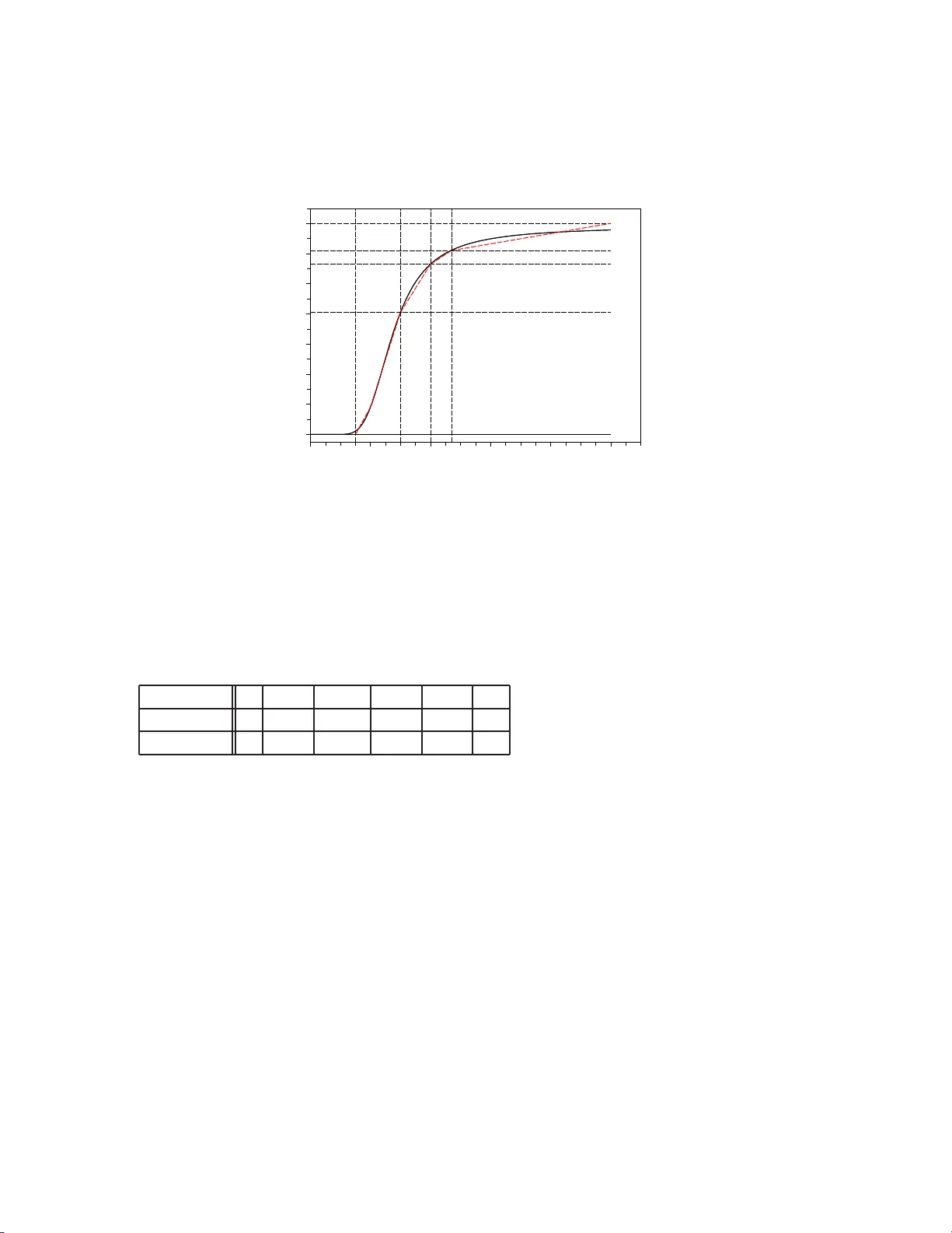
Piecewise linear car-following mo deling Nadir F arhi Universit´ e Paris-Est, IFSTT AR, GRETTIA, F-93166 N oisy-le-Gr and, F r anc e. Abstract W e presen t a traffic mo del that extends the linear car-following model as we ll as the min- plus traffic mo del (a mo del based on the min-plus a lgebra). A discrete-time car-dynamics describing the traffic on a 1- lane road without passing is interprete d a s a dynamic program- ming equation of a stochastic optimal con tro l problem of a Marko v c hain. This v ariatio na l form ulation p ermits to c haracterize the stability of the car-dynamics and to calculte the stationary regimes when the y ex ist. The model is based on a piecewis e linear appro ximation of the fundamen tal traffic diagr a m. Keywor ds: Car-follow ing mo deling, Optimal con t r ol, V ariational formulations. 1. In tro duction Car-follow ing mo dels are microscopic traffic mo dels tha t describe the car-dynamics with stim ulus-resp onse eq uations expressing the driv ers’ b eha vior. Eac h driv er resp onds, by c ho os- ing its sp eed or acceleration, to a giv en stim ulus that can b e comp osed of many f actors suc h as in ter-veh icular distances, relative v elo cities, instantaneous v elo cities, etc. W e presen t in this article a car-following mo del that extends t he linear car-following mo del [5, 21, 14, 13], as w ell as the min-plus traffic mo del [27]. The v ehicular traffic on a 1-lane road without passing is des crib ed b y discrete-time dy- namics, whic h are interpreted as dynamic prog ramming equations asso ciated to sto chastic optimal control problems of Mark ov c hains. The discrete-time v aria t io nal formulation w e mak e here is similar to the time-con tin uo us one used b y Da ganzo and Geroliminis [7] to sho w the existenc e of a conca v e macrosc opic fundamen tal diagram. W e are concerned in this article b y microscopic traffic mo deling with a Lag rangian de- scription of the traffic dynamics, where the function x ( n, t ), giving the p osition of car n at time t ( o r the cum ulated distance tra v eled b y a car n up to time t ), is used. In the macro- scopic kinematic traffic mo deling, Eulerian descriptions of the traffic dynamics are usually used, with the function n ( t, x ) giving the cum ulated n um b er of cars passing through p osition x up to time t (whic h coincides with the Mosco witz function [6] in the case of tr a ffic without passing). The com bination o f a conserv at io n law with an equilibrium la w giv es the we ll kno wn first order t r affic mo del of Lighthill, Whitham and Ric hards [26, 29]. Email addr ess: n adir.far hi@ifsttar.fr (Nadir F a rhi) In this in tro duction, we first notice that the same a pproac h used in macroscopic traffic mo deling, com bining a conserv ation la w with a n equilibrium law, can b e used to deriv e microscopic traffic mo dels. By this, w e intro duce car- follo wing mo dels and giv e a review on basic and most imp ortant existing ones. In particular, w e recall the linear and the min-plus car-followin g mo dels, whic h are particular cases of the mo del w e presen t here. Finally , we recall a theoretical result on non-expansiv e and connected dyn amic systems whic h w e need in our dev elopmen ts, and give the outline of this article. The first order partial deriv ativ e o f the function x ( n, t ) in time, denoted ˙ x ( n, t ) express es the v elo cit y v ( n, t ) of car n at t ime t . The first order differen tiation of x ( n, t ) in the car n um b ers ∆ x ( n, t ) expresses the in v erse of the inter-v ehicular distance y ( n, t ) = x ( n − 1 , t ) − x ( n, t ) b etw een cars n and n − 1 at time t . Th e equality of the se cond deriv ativ es ∆ ˙ x ( n, t ) and ˙ ∆ x ( n, t ) giv es then the following conserv ation law of distance. ˙ y ( n, t ) = − ∆ v ( n, t ) . (1) If w e assume that a fundamental diagram V e , giving the ve lo cit y v as a function of the in ter-v ehicular distance y ( v = V e ( y )) at the stationary traffic, exists, and that the diagram V e holds also on the transien t traffic, then w e ha ve ˙ y ( n, t ) = ˙ v ( n, t ) /V ′ e ( y ) , (2) where V ′ e ( y ) denotes the deriv ativ e of V e with resp ect to y . By com bining (1) and (2) w e obtain the mo del: ˙ v ( n, t ) = − V ′ e ( y ( n, t ))∆ v ( n, t ) . (3) (3) is a car- follo wing mo del that giv es the acceleration of car n at time t as a resp onse to a stim ulus comp osed of the relative sp eed ∆ v ( n, t ) and the term V ′ e ( y ( n, t )). F or example, if V e ( y ) = v 0 exp − a/y , where v 0 denotes the free (or desired) ve lo cit y , and a is a parameter, then V ′ ( y ) = aV ( y ) /y 2 and (3) giv es a particular case of the Gazis, Herman, and Rothery mo del [13]. The simplest car-follo wing mo del is the linear one, where the car dynamics are written ˙ x n ( t + T ) = a ( x n − 1 ( t ) − x n ( t )) + b, (4) where T is the reaction time, a is a s ensitivit y parameter, and b is a constant. That mo del can b e deriv ed from (3) with a linear fundamen tal diagram V e . The stabilit y of the linear car-followin g mo del (4) and the existence of a stationary regime hav e b een treated in [21]. Almost all car follow ing mo dels are based on the assumption of the existence of a b e- ha vioral law V e . The latter has b een tak en linear in [1 7, 21], logarithmic in [16], exp onen tia l in [2 8], and with more complicated fo rms in other w o rks. Bando et al. [3] used the sigmiudal function V e ( y ) = tanh ( y − h ) + tanh ( h ) , (5) where tanh denotes the hyperb olic tangent f unction, and h is a constan t. 2 Kerner and Konh¨ auser[24], Hermann and Kerner [22], and t hen Lenz et al.[25], a nd Ho ogendo orn et al. [23] hav e used the function V e ( y ) = v 0 (  1 + exp  1 , 000 γ · y − 10 2 . 1  − 1 − 5 . 34 · 10 − 9 ) , (6) where free v elo cit y v 0 and γ are parameters es timated from data. In [25], γ is tak en equal to 7 . 5. See also [1 9 , 20, 30]. The min-plus traffic mo del [27] is a microscopic discrete-time car- follo wing mo del based on the min- plus algebra [2]. It consists in the follow ing dynamics. x n ( t + 1) = min { x n ( t ) + v 0 , x n − 1 ( t ) − σ } , (7) where v 0 is the free velocity a nd σ is a safet y dis tance. The idea of the mo del (7) is that the car dy namics is linear in the min-plus algebra [2], where the addition is the op eration “min” and the pro duct is the standar d addition “+”. In [27], the dynamic syste m (7) is written in min-plus notations x ( t ) = A ⊗ x ( t − 1), where A is a min-plus matrix and ⊗ is the min-plus pro duct o f matrices. It is then pro v ed that the a v erage grow th rate ve ctor per time unit of the system, defined b y χ = lim t →∞ x ( t ) /t satisfies χ = ( ¯ v , ¯ v , · · · , ¯ v ), where ¯ v is the unique min-plus eigenv alue of the matrix A , inte rpreted as the stationary car-sp eed. The fundamen tal diag ram is then obtained ¯ v = min( v 0 , ¯ y − σ ) (8) ¯ q = min( v 0 ¯ ρ, 1 − σ ¯ ρ ) , (9) where ¯ y , ¯ q and ¯ ρ denote resp ectiv ely the equilibrium inter-v ehicular distance, car-flow and car-densit y . In (7), for t ≥ 0, if x n − 1 ( t ) − x n ( t ) > v 0 + σ , then the dynamics is x n ( t + 1) − x n ( t ) = v 0 . If x n − 1 ( t ) − x n ( t ) ≤ v 0 + σ then the dynamics is x n ( t + 1) − x n ( t ) = x n − 1 ( t ) − x n ( t ) − σ . Therefore, (7) is linear in b oth phases of free and congested tra ffic. The min-plus mo del (7) p ermits to distinguish tw o phases in whic h the traffic dynamics is linear, but with a sensitivit y parameter ( a in (4)) equals to 1 for eac h phase. The linear mo del (4) is not constrained in the sensitivit y parameter v alue, but it p ermits the modeling of o nly one traffic phase. The mo del w e presen t here extends (4 ) and (7) in a w a y that an arbitrary n um b er of t r affic phases can b e modeled, with flexibilit y in the sens itivit y parameter v alue on eac h phase. F or our mo del, w e apply a similar but more general appro a c h than the min-plus one used to analyze the dynamic system (7). In deed, the dynamics ( 7 ) is additive homog eneous of degree one 1 and is monotone 2 . It is then non expans iv e 3 [4]. The stability of the dynamic 1 A dyna mic system x ( t ) = f ( x ( t − 1)) is additive homogeneo us of degree 1 if f is so, tha t is if ∀ x ∈ R n , ∀ λ ∈ R , f ( λ + x ) = λ + f ( x ). 2 A dyna mic system x ( t ) = f ( x ( t − 1)) is monotone if f is so, that is if ∀ x 1 , x 2 ∈ R n , x 1 ≤ x 2 ⇒ f ( x 1 ) ≤ f ( x 2 ), where the order ≤ is p oint wise in R n . 3 A dynamic sys tem x ( t ) = f ( x ( t − 1)) is non expansive if f is so, that is if ther e exists a norm || · || in R n such that ∀ x 1 , x 2 ∈ R n , || f ( x 2 ) − f ( x 1 ) || ≤ || x 2 − x 1 || . 3 system (7) is th us guaran teed from its non expansiv eness. Moreov er, (7) is connected (or comm unicating) 4 [11, 12]. An imp orta nt result from [18, 11] (Theorem 1 b elo w) p ermits the analysis of non expansiv e and connected dynamic systems. Theorem 1. [18, 1 1] If a dynamic system x ( t ) = f ( x ( t − 1)) is non exp an sive and c onne cte d, then the additive eigenvalue pr oblem ¯ v + x = f ( x ) admits a solution ( ¯ v, x ) , wher e x is defin e d up to an addi tive c onstant, not ne c essarily in a unique way, an d ¯ v ∈ R n is unique. Mor e o v e r, the dyna m ic system admits an aver ag e gr ow th r ate ve ctor χ , wh i c h is unique (ind e p endent of t he initial c ondition) a n d given by χ ( f ) = t ( ¯ v , ¯ v , · · · , ¯ v ) . The model treated in this article can b e seen as an extension of the min-plus mo del (7) . In Section 2, we presen t the model. It is called pie c ewi s e line ar c ar-fo l lowi n g mo del b ecause it is based on a piecewise linear fundamen ta l diagram V e . The mo del describes the traffic of cars on a ring road of one lane without passing. The s tabilit y conditions of the dynamic system describing the traffic are determined. Under those conditions, the car- dynamics are in terpreted as a dynamic programming equation (DPE) asso ciated to a sto c hastic optimal con trol problem of a Mark o v c hain. The DPE is solve d analytically . W e sho w that t he individual b eha vior la w V e supp osed in the mo del is realized on the collectiv e stationary regime. F inally , the effect of t he stabilit y condition on the s hap e of the fundamen tal diagra m is sho wn. In section 3, w e giv e equiv a len t results of those given in section 2 for the traffic on an “op en” ro ad (a highw ay stretc h for example), and conclude with an example, where w e sim ula t e the transien t traffic, basing o n a piecewis e linear appro ximation of the diagram (6) . In App endix B, w e giv e more details on t he duality in traffic mo deling, of using the functions n ( t, x ) , x ( n, t ) and t ( n, x ), where t ( n, x ) denotes the time of passage o f the n th car b y p osition x . 2. Piecewise linear car follo wing mo del The b eha vioral law V e is an increasing curv e b ounded by the free sp eed v 0 . Moreo ve r, V e ( y ) = 0 for y ∈ [0 , y j ] where y j denotes the jam inter-v ehicular distance. W e prop ose here to appro ximate the curve V e with a piecewis e-linear curv e V e ( y ) = min u ∈U max w ∈W { α uw y + β uw } , (10) where U and W are t w o finite sets of indices . Since V e is increasing, we hav e α uw ≥ 0 , ∀ ( u, w ) ∈ U × W . W e are intere sted here on the disc rete-time first-or der dynamics x n ( t + 1) = x n ( t ) + min u ∈U { α u ( x n − 1 ( t ) − x n ( t )) + β u } , (11) 4 An a dditive homogeneous of degree 1 and monotone dynamic system x ( t ) = f ( x ( t − 1)) with x ∈ R n is connected if its as socia ted gr aph is strongly connected. The graph a sso ciated to that dynamic system is the graph with n no des and who s e arcs a re determined as follows. There exists a n arc from a no de i to a no de j if l im ν →∞ f j ( ν e i ) = ∞ , where e i denotes the i th vector of the canonic bas is of R n . 4 and x n ( t + 1) = x n ( t ) + min u ∈U max w ∈W { α uw ( x n − 1 ( t ) − x n ( t )) + β uw } . (12) It is clear that (12) extends (11). The model (12) is also an e xtension of b oth linear mo del (4) and min-plus mo del ( 7 ). In this article, w e c haracterize the stability of the dynamics (12), calculate the stationary regimes, s ho w tha t the fundamen tal diagrams a re effectiv ely realized at the stationary regime, and a na lyze the transien t traffic. W e will distinguish t w o cases : T r a ffic on a ring road and traffic on an “op en” road. 2.1. T r affic on a rin g r o ad W e follo w here the mo deling of [27]. L et us consider ν cars mo ving a one-lane ring road in one direction without passing. W e assume that the cars ha v e the same length that w e tak e here as the unity of distance. The road is assumed to b e of size µ ; that is, it can con ta in at most µ cars. The car densit y on the road is thus ρ = ν /µ . Sto chastic o p timal c ontr ol mo del W e consider here the car dynamics (1 1). That is to sa y that each car n maximizes its v elocity at time t under the constrain ts x n ( t + 1) ≤ x n ( t ) + α u ( x n − 1 ( t ) − x n ( t )) + β u , ∀ u ∈ U . (13) Eac h constrain t of (13) b ounds the v elo cit y x n ( t + 1) − x n ( t ) b y a sum of a fixed term β u and a term dep ending linearly on the in ter-v ehicular distance. Let us first not ice that (1 1), o n the ring road, is written x n ( t + 1) = x n ( t ) + min u ∈U { α u ( x n − 1 ( t ) − x n ( t )) + β u } , for n ≥ 2 , x 1 ( t + 1) = x 1 ( t ) + min u ∈U { α u ( x n ( t ) + µ − x 1 ( t )) + β u } , whic h can also b e written x n ( t + 1) = min u ∈U { (1 − α u ) x n ( t ) + α u x n − 1 ( t ) + β u } , for n ≥ 2 , x 1 ( t + 1) = min u ∈U { (1 − α u ) x 1 ( t ) + α u x n ( t ) + α u ν /ρ + β u } . Let us denote b y M u , u ∈ U the family of matrices defined b y M u =      1 − α u 0 · · · α u α u 1 − α u 0 . . . . . . . . . 0 0 α u 1 − α u      , and b y c u , u ∈ U , the family of v ectors de fined b y c u = t [ α u ν /ρ + β u , β u , · · · , β u ] . 5 The dynamics (11) are then written : x n ( t + 1) = min u ∈U { [ M u x ( t )] n + c u n } , 1 ≤ n ≤ ν . (14) The system (14) is additiv e homog eneous of degree 1 b y the definition of the matrices M u , u ∈ U . It is monotone under the condition that all the comp onen ts of M u , u ∈ U are non negativ e, whic h is equiv alent to α u ∈ [0 , 1] , ∀ u ∈ U . Henc e, under that condition, the system (14) is non expansiv e. Moreo v er, the matrices M u , u ∈ U are sto c hastic 5 . Those matrices can then be se en as transition matrices of a con tr o lled Mark ov chain, where the set of c on trols is U . The connect- edness of the sys tem (14), as defined in the previous section, is related to the irreducibilit y of the Mark o v chain with transition matrices M u , u ∈ U . It is easy to chec k that (1 4) is connected if and only if ∃ u ∈ U , α u ∈ (0 , 1]; see Appendix A for t he proo f . That condition is in terpreted in term of tra ffic by sa ying that ev ery car mo v es b y taking into accoun t the p osition of the car ahead. Consequen tly , under the condition ∀ u ∈ U , α u ∈ [0 , 1 ] and ∃ u ∈ U , α u ∈ (0 , 1 ], the dynamic sy stem (1 4) is no n expansiv e a nd is connected. Therefore, b y Theorem 1, w e conclude that the a dditiv e eigenv alue problem ¯ v + x n = min u ∈U { [ M u x ] n + c u n } , 1 ≤ n ≤ ν , (15) describing the stationary regime of the dynamic system (14), admits a solution ( ¯ v , x ), where x is defined up to a n additiv e constan t, not necessarily in a unique w a y , and ¯ v ∈ R n is unique. Moreo ver, the dynamic system admits a unique a ve rage gro wth rate p er time unit χ , whose comp onents are a ll equal and coincide with ¯ v . The a v erage gro wth rate p er time unit χ of the system (14) is in terpreted in t erm of traffic as the s tationary car- velocity . The additiv e eigen v ector x gives the asymptotic dis tribution of cars on the ring . x is giv en up to an additive constant, sinc e the car - dynamics ( 1 4) is additiv e homogeneous of degree 1. That is to say that if ( ¯ v , x ) is a solution of (15) then ( ¯ v , e + x ) is also a solution for (15), fo r ev ery constan t e ∈ R . Let us now g iv e an in terpretation of the mo del in term o f ergo dic sto c ha stic optimal con trol. Indeed, ( 1 5) can b e seen as a dynamic programming equation of an ergo dic sto c hastic optimal con trol problem of a Mark o v chain with tra nsition matrices M u , u ∈ U and costs c u , u ∈ U , and with a se t of states N = { 1 , 2 , · · · , ν } . The stochas tic optimal control problem of the c hain is written min s ∈S E ( lim T → + ∞ 1 T T X t =0 c u t n t ) , (16) where S is a set of feedbac k strategies on N . A strategy s ∈ S asso ciates t o ev ery state n ∈ N a control u ∈ U (that is u t = s ( n t )). The follo wing result giv es one solution ( ¯ v , x ) for the dynamic programming equation (15). 5 W e mean here M u ij ≥ 0 , ∀ i , j and P j M u ij = 1 , ∀ i . 6 Theorem 2. The system (15) admits a solution ( ¯ v , x ) give n by: ¯ v = min u ∈U { α u ¯ y + β u } , x = t [0 ¯ y 2 ¯ y · · · ( ν − 1) ¯ y ] . Pr o of. First, b ecause of the symmetry of the sy stem (1 5), it is na t ural that the asymptotic car-p ositions x n , 1 ≤ n ≤ ν are uniformly distributed o n the r ing , a nd that the optimal strategy is independen t of the state x . Let us pro ve it. Let ¯ u ∈ U b e defined by α ¯ u ¯ y + β ¯ u = min u ∈U { α u ¯ y + β u } = ¯ v . Let x b e the v ector giv en in Theorem 2. Then ∀ n ∈ { 1 , 2 , · · · , ν } we hav e [ M ¯ u x ] n + c ¯ u n = ( α ¯ u ¯ y + β ¯ u ) + x n = min u ∈U ( α u ¯ y + β u ) + x n = min u ∈U { [ M u x ] n + c u n } = ¯ v + x n . In term of traffic, T heorem 2 show s that the car- dynamics is stable under the condition α u ∈ [0 , 1], and the a v erage car sp eed is giv en b y the additive eigen v alue of the asymp- totic dynamics in the case where the syste m is connected. Moreo v er, it a ffirms that the fundamen tal diagram supposed in the mo del is realized at the stat io nary regime. ¯ v = min u ∈U { α u ¯ y + β u } , (17) ¯ q = min u ∈U { α u + β u ¯ ρ } . (18) It is imp ortan t to note here that, up to the assumption α u ∈ [0 , 1] , ∀ u ∈ U , ev ery concav e curv e V e or Q e can b e appro ximated with (17) or (18). Indeed, approx imating fundamen tal diagrams us ing those fo r mulas is nothing but computing F enc hel transforms; see [6 , 1]. More precisely , if w e denote b y V the set V = { β u , u ∈ U } and define the function g b y: g : V → R v = β u 7→ − α u , then q = Q e ( ρ ) = min v ∈V ( ρv − g ( v )) = g ∗ ( ρ ) , where g ∗ denotes the F enche l transform of g . Finally , w e note that the min-plus linear model is a particular case of the mo del presen ted in this se ction, where U = { u 1 , u 2 } with ( α 1 , β 1 ) = (0 , v ) a nd ( α 2 , β 2 ) = (1 , − σ ). In this case, the fundamen tal traffic diagram is approximated with a piece wise linear curv e with t w o segmen ts. 7 Sto chastic g a me mo del W e consid er in this section the car dy namics (12), again with the assumption ∀ ( u, w ) ∈ U × W , α uw ∈ [0 , 1] and ∃ ( u, w ) ∈ U × W , α uw ∈ (0 , 1]. The dynamic system (12) is in terpreted as a stochastic dynamic programming equ ation ass o ciated to a stochastic game problem on a con tro lled Mark ov c hain. As abov e, a generalized eigenv alue problem is solv ed. The extension w e ma ke here approximates non concav e fundamental diag rams. In term o f traffic, w e tak e in to account the drive rs’ b ehavior c hang ing from lo w densitie s to high ones. The difference b et w een these tw o situations is that in lo w densities, driv ers, mo ving, or b e ing able to move with high v elo cities, they try to lea ve large safety dis tances b et w een each other, so the safet y distance s are maximized; whilst in high densities, drivers , mo ving, or having to move with lo w v elo cities, they try to lea ve small safet y distances b et w een each other in order to a v o id jams; so they minimize safety distances. T o illustrate this idea, let us consider the follo wing tw o dynamics of a giv en car n . x n ( t + 1) = min { x n ( t ) + v , x n − 1 ( t ) − σ } , (19) x n ( t + 1) = min { x n ( t ) + v , max { x n − 1 ( t ) − σ, ( x n ( t ) + x n − 1 ( t )) / 2 }} . (20) The dynamics (19) is a min-plus dynamics whic h grossly tell that car s mo ve with t heir desired v elo cit y v at the fluid regime and they k eep a safet y distance σ at the congested regime. The dynamics (20) distinguishes t w o situations at the congested regime: • In a relative ly lo w densit y situation where the cars are separated b y a distance that equals at least to 2 σ w e ha ve max { x n − 1 ( t ) − σ, ( x n ( t ) + x n − 1 ( t )) / 2 } = x n − 1 ( t ) − σ. • In a high densit y situation, where the cars a re separated by distances less than 2 σ w e ha v e max { x n − 1 ( t ) − σ, ( x n ( t ) + x n − 1 ( t )) / 2 } = ( x n ( t ) + x n − 1 ( t )) / 2 . In this case, we accept the cars mo ving close r but b y redu cing the approac h sp eed in order to a void collisions. This is realistic. The situation w e ha v e considered in (20) is realistic and v ery simple, but, it cannot be obtained without in tro ducing a maximum op erator in the d ynamics (i.e. w ith only minim um op erators). Indeed, with only minim um op erators the approa c h is mec hanically reduced with t he incre asing of the car-densit y (in fa ct this is the concav eness of the fundamental diagram). Because of the realness of such sce narios, w e think that the fundamen tal traffic diagram should be comp osed of t wo pa r t s, a conca v e part at the fluid regime, and a conv ex part at the congested regime. The dynamics (1 2) g eneralizes this idea. The dynamics (12) can be written x n ( t + 1) = min u ∈U max w ∈W { [ M uw x ( t )] n + c uw n } , 1 ≤ n ≤ ν , (21) 8 where M uw =      1 − α uw 0 · · · α uw α uw 1 − α uw 0 . . . . . . . . . 0 0 α uw 1 − α uw      , and c u = t [ α uw ν /ρ + β uw , β uw , · · · , β uw ] . Similarly , w e can easily c heck that the dynamic system (21 ) is non expansiv e unde r t he condition α uw ∈ [0 , 1] , ∀ ( u, w ) ∈ U × W . Its stabilit y is thus gua r a n teed under that condition. If, in addition, ∃ ( u, w ) ∈ U × W , α uw ∈ (0 , 1], then the syste m is connected. In this case, w e get the same results as in Theorem 2. That is, the eigen v alue problem ¯ v + x n = min u ∈U max w ∈W { [ M uw x ] n + c uw n } , 1 ≤ n ≤ ν (22) admits a solution ( ¯ v, x ) giv en b y: ¯ v = min u ∈U max w ∈W { α uw ¯ y + β uw } , x = t [0 ¯ y 2 ¯ y · · · ( ν − 1) ¯ y ] . Moreo v er, the dynamic system (21) admits a unique a ve rage growth rate v ector χ , whose comp onen ts are all equal to ¯ v . The car-dynamics is then stable under the condition ∀ ( u, w ) ∈ U × W , α uw ∈ [0 , 1], a nd the a v erage car sp eed is giv en b y the additiv e eigen v alue o f the asymptotic dynamics in the case where the sys tem is connected (that is, if ∃ ( u, w ) ∈ U × W , α uw ∈ (0 , 1]) . The b ehavior la w supposed in the mo del is realized at the stationary regime. ¯ v = min u ∈U max w ∈W { α uw ¯ y + β uw } , (23) ¯ q = min u ∈U max w ∈W { α uw + β uw ¯ ρ } . (24) In term of sto c hastic optimal control, the system (22) can b e seen as a dynamic pro gram- ming equation asso ciated to a sto c hastic game, with t w o pla y ers, on a Mark o v c hain. The set of states of the chain is again N = { 1 , 2 , · · · , ν } . The chain is con trolled by t w o pla y ers, a minimizer o ne with a finite set U o f con tro ls, and a maximizer one with a finite set W of con trols. The transitions and the costs of the c hain are giv en b y the matrices M uw and the v ectors c uw , ( u, w ) ∈ U × W define d ab o v e. The sto c ha stic optimal control problem is min max | s ∈S E ( lim T → + ∞ 1 T T X t =0 c u t w t n ( t ) ) , (25) 9 where S is the set of strategies assoicating to ev ery state n ∈ N a couple of commands ( u, w ) ∈ U × W . It is a ssumed here that the maximizer kno ws at each step the decision of the minimizer. W e no w giv e a conse quence of the stability condition α uw ∈ [0 , 1] , ∀ ( u, w ) ∈ U × W , on the shap e of t he fundamen tal diagrams (23) and (24). As show n in Figure 1, where w e ha v e dra wn the fundamen tal diagram (6) (with v 0 = 14 meter b y half second, and γ = 7 . 5), the stabilit y condition puts the curv es (23) and (24) in sp ecific resp ectiv e regio ns in the plan. Indeed, for the diagram (23), if w e assume that V e is b ounded b y v 0 , V e ( y ) = 0 , ∀ y ∈ [0 , y j ], 0 20 40 60 80 100 0 5 10 15 Inter−vehicular distance (meter) Car−velocity (meter by half second) 0.0 0.1 0.2 0.3 0.4 0.5 0.6 0.7 0.8 0.9 1.0 0.0 0.1 0.2 0.3 0.4 0.5 0.6 0.7 0.8 0.9 1.0 car−density normalized car−flow Figure 1: The effect of the stability condition α uw ∈ [0 , 1] on the sha pe of the fundamental diagram. and that V e is con tin uous (and increasing), then starting by the po int ( y j , 0), one cannot join an y p oin t ab o v e the line passing by ( y j , 0) and having the slop e 1, with an y sequence of segmen ts of slop es α uw ∈ [0 , 1]. W e can write V e ( y ) ≤ max(0 , min( v 0 , y − y 0 )) . Similarly , o n the dia g ram (24), if w e assume that Q e is contin uous and Q e ( ρ ) = 0 , ∀ ρ ∈ [ ρ j , 1], then going bac k f rom the p oint ( ρ j , 0), one cannot attain an y point abov e the line passing b y ( ρ j , 0) and (0 , 1), with a sequence of segmen ts ha ving their ordinates at the origin ( α uw ) in [0 , 1]. W e can write Q e ( ρ ) ≤ max (0 , min( v 0 ρ, 1 − ρ/ρ j )) . 3. T raffic on an op en road W e study in this section the traffic on an op en road with one lane and without pass ing. W e are intere sted in the follo wing dynamic s. x 1 ( t + 1) = x 1 ( t ) + v 1 ( t ) , x n ( t + 1) = min u ∈U max w ∈W { x n ( t ) + α uw [ x n − 1 ( t ) − x n ( t )] + β uw } . (26) 10 If w e denote b y M uw the matrices M uw =      1 0 · · · 0 α uw 1 − α uw 0 . . . . . . . . . 0 0 α uw 1 − α uw      , and b y c uw ( t ) the v ectors c uw ( t ) = t [ v 1 ( t ) , β uw , · · · , β uw , β uw ] , for ( u, w ) ∈ U × W and t ∈ N , then the dynamic sys tem (26) is written x n ( t + 1) = min u ∈U max w ∈W { [ M uw x ( t )] n + c uw n } , 1 ≤ n ≤ ν . (27) It is easy to c hec k t ha t the dynamic system (27) is a dditiv e homogeneous of degree 1, and is monotone unde r the condition ∀ ( u, w ) ∈ U × W , α uw ∈ [0 , 1]. Therefore, under that condition, (27) is non exp ansiv e. How ev er, (27) is not connected for ev ery ( u, w ) ∈ U × W . W e will b e in terested here, in particular, in the stationary regime, where v 1 ( t ) reac hes a fixed v alue v 1 . F or this case, the eigen v a lue problem asso ciated to (2 6 ) is ¯ v + x 1 = x 1 + v 1 , ¯ v + x n = min u ∈U max w ∈W { x n + α uw [ x n − 1 − x n ] + β uw } . (28) The system (28) is also written ¯ v + x n = min u ∈U max w ∈W { [ M uw x ] n + c uw n } , 1 ≤ n ≤ ν , (29) where c uw = t [ v 1 , β uw , · · · , β uw , β uw ] . Then w e hav e the following result. Theorem 3. F or al l y ∈ R satisfying min u ∈U max w ∈W ( α uw y + β uw ) = v 1 , the c ouple ( ¯ v , x ) is a solution for the system ( 2 8), wher e ¯ v = v 1 and x is given up to a n additive c onstant by x = t [( n − 1) y , ( n − 2) y , · · · , y , 0] . (30) Pr o of. The pro of is similar to that of Theorem 2. Let y ∈ R satisfying min u ∈U max w ∈W ( α uw y + β uw ) = v 1 . Let ( ¯ u, ¯ w ) ∈ U × W suc h that α ¯ u ¯ w y + β ¯ u ¯ w = v 1 . Let x b e g iv en b y (30). Then ∀ n ∈ { 1 , 2 , · · · , ν } w e hav e [ M ¯ u ¯ w x ] n + c ¯ u ¯ w n = ( α ¯ u ¯ w y + β ¯ u ¯ w ) + x n = min u ∈U max w ∈W ( α uw y + β uw ) + x n = min u ∈U max w ∈W [ M uw x ] n + c uw n = v 1 + x n . 11 W e can easily che c k that for ( u, w ) ∈ U × W suc h tha t α uw = 0 and β uw = v 1 , ev ery in ter- v ehicu lar distance y ∈ R satisfies t he condition min u ∈U max w ∈W ( α uw y + β uw ) = v 1 . Th us, suc h couples ( u , w ) do not count for t ha t condition. Theorem (3) can then b e announced differen t ly . Let us denote by W u for u ∈ U the family of index sets W u = { w ∈ W , ( α uw , β uw ) 6 = (0 , v 1 ) } , and b y ˜ y the asymptotic a v erage car-inter-v ehicular distance: ˜ y = max u ∈U min w ∈W u v 1 − β uw α uw , (31) where w e use the con v ention a/ 0 = + ∞ if a > 0 and a/ 0 = −∞ if a < 0. Then Theorem 3 tells simply that if ˜ y ∈ R (i.e. −∞ < ˜ y < + ∞ ), then the dynamic system (28) admits a solution ( ¯ v , x ) where ¯ v = v 1 is unique, a nd where x is not necessarily unique and is giv en up to an additiv e constant b y x = t [( n − 1) ˜ y, ( n − 2) ˜ y , · · · , ˜ y , 0] . Non-uniform a symptotic car-distributions can also b e o bta ined. Let us clarify the follo w- ing three cases. • If ∃ u ∈ U , ∀ w ∈ W u , α uw = 0 and β uw < v 1 , then ˜ y = + ∞ . In this case, the distance b et w een the first car and the other cars increases o ve r time and go es to + ∞ . The asymptotic car-distribution on the road is no t uniform. • If ∀ u ∈ U , ∃ w ∈ W u , α uw = 0 a nd β uw > v 1 , then ˜ y = −∞ . In this case, the first car is passed b y all other cars, and the distance b et w een t he first c ar and the other cars increases o v er time and go es to + ∞ . The asymptotic car-distribution on the road is not uniform. • If ∀ u ∈ U , ∀ w ∈ W u , α uw = 0 and if min u ∈U max w ∈W u β uw = v 1 , then for all x ∈ R ν , ( v 1 , x ) is a solutio n for the system (2 8). In this case, ev ery distribution of the cars mo ving all with the constan t v elocity v 1 is stationary . The form ula (31) is the fundamental traffic diagram expressing the a ve rage inter-v ehicular distance as a function of the car sp eed at the stationary regime. In t he case where only a minimum op erator is used in (26), the form ula (31) is reduced to the con v ex fundamen t a l diagram y = max u ∈U v 1 − β u α u . (32) Example 1 . In order to understand t he tra nsien t t r a ffic, let us sim ulate the car-dynamics (26). W e tak e as the time unit half a second (1 /2 s), a nd as the distance unit 1 meter (m). The parameters of the mo del are determined by appro ximating the b eha vior law (6), with a free v elocity v 0 = 14 m/ 1/2s ( which is ab out 100 km/h) and γ = 7 . 5 as in [25]; see Figur e 2. 12 0 20 40 60 80 100 0 2 4 6 8 10 12 14 Inter−vehicular spacing (meter) Car−velocity (meter / half second) Figure 2: Approximation of the b ehavioral law (6 ) with a piecewise linear cur v e. The b eha vior la w is approxim ated b y the follow ing piecewis e linear curve of s ix segmen ts. ˜ V ( y ) = max { α 1 y + β 1 , min { α 2 y + β 2 , α 3 y + β 3 , α 4 y + β 4 , α 5 y + β 5 , α 6 y + β 6 }} , where the parameters α i and β i for i = 1 , 2 , · · · , 6 are giv en b y Segmen ts 1 2 3 4 5 6 α i 0 0.54 0.32 0.13 0.34 0 β i 0 - 8.1 -1.47 6.11 10.6 14 W e sim ulate the piecewise linear car-following mo del asso ciated to the appro ximation ab o v e. x 1 ( t ) = x 1 ( t − 1) + v 1 ( t ) , x n ( t ) = x n ( t − 1) + ˜ V ( x n − 1 ( t − 1) − x n ( t − 1 )) . (33) The v elo cit y of the first car v 1 ( t ) , t ≥ 0 is v aried in t he t ime interv al [0 , 1000], then fixe d to the free v elo city v 0 = 14 m/ 1/2s in the time in terv al [1 000 , 3000], and finally fixed on a v elo city t hat exceeds v 0 in the r emaining time [3000 , 7200]. The a ve rage in ter-v ehicular distance is then computed at ev ery time t , and the results are sho wn in Figure 3. The simple sim ulation w e made here p ermits to ha ve a n ide a of the traffic in the transien t regime. Figure 3 shows how the a v erage of the inter-v ehicular distance is c hanged due to a changing in the v elocity of the first car. In the righ t side of F igure 3, w e compare the fundamen tal la w assum ed in the mo del with the diagram giving the aver age inte r-v ehicular distance (with respect to the num b er of cars) function of the velocity of the first car (a kind of macroscopic fundamen tal diagram). W e observ e that lo ops are obtained on that diagram in t he tra nsien t traffic. The lo ops are in terpreted b y the fact t ha t once the v elo cit y of the first car is temp orarily stationary , the v elo cities of the follow ing cars, and th us also 13 0 1000 2000 3000 4000 5000 6000 7000 0 20 40 60 80 100 120 140 Time (1/2 s) 1st car vel. and aver. inter−car dist. 0 2 4 6 8 10 12 14 16 18 20 22 0 20 40 60 80 100 120 140 Velocity of the first car (m / 1/2 s) Average car inter−distance (m) Figure 3: Sim ulation r esults. On the left-side: the first car velo cit y (solid line), a nd the av erage inter-vehicular distance (dash line) functions of time. On the r igh t side: the approximation of the b ehavior law (6) (dash line), and the av erage in ter-vehicular distance obtained by sim ulation in function of the velo cit y of the first car (solid line). the a v erage v elo city of the cars, make some time to attain the first car v elo city . It can also b e in terpreted b y sa ying t hat ev en though the cars hav e, individually , t he same r esponse to a c hang ing in in t er- v ehicular distance; their collectiv e resp onse dep ends on whether the in ter-v ehicular distance is increasing or decreasing. The apparition of suc h lo ops is due to the reaction time o f driv ers. It can also b e related to the n um b er of an ticipation cars in case of m ulti-an ticipativ e mo deling. Ho w ev er, one ma y measure on a giv en section, different car-flo ws for the same car dens it y (or o ccupancy rate) dep ending on the traffic acceleration or decele ration, and interpre t it as the h ysteresis phe nomenon [8, 31, 32, 15 ]. 4. Conclusion W e propo sed in this a rticle a car - follo wing mo del whic h exte nds the linear car-f ollo wing mo del as w ell as the min-plus mo del. The stability and the stationary regimes of the mo del are characterized thanks to a v ar iational f o rm ulat io n of the car-dynamics. This formulation, although already made with con tinuous -time mo dels, it p ermits to clarify the stim ulus- resp onse pro cess in microscopic discrete-time traffic mo dels, a nd to inte rpret it in term of sto c hastic optimal con trol. Among the imp ortant questions to b e treated in the future, the impacts of heterogeneit y and an ticipation in driving, on t he transient and stationary traffic regimes, based on the mo del prop osed in this article. App endix A. Connectedness of system (14) Let x ∈ R ν . W e denote b y h : R ν → R ν the op erator defined b y h ( x ( t )) = x ( t + 1), where x n ( t + 1), for 1 ≤ n ≤ ν are giv en by the definition of the system (14). That is x n ( t + 1) = min u ∈U { [ M u x ( t )] n + c u n } , 1 ≤ n ≤ ν . 14 • If ∃ u ∈ U , suc h that α u ∈ (0 , 1], then for all n ∈ { 1 , 2 , · · · , ν } , there exists an a rc, on t he graph associated to h , going from n − 1 to n ( n being cyclic in { 1 , 2 , · · · , ν } ). Indeed, x n ( t + 1) = ( 1 − α u ) x n ( t ) + α u x n − 1 ( t ) + β u . Then since α u > 0, w e get: lim ν →∞ h n ( ν e n − 1 ) = lim ν →∞ [ α u ν + β u ] = ∞ . where e n − 1 denotes the ( n − 1 ) th v ector of the canonic basis o f R ν . The refore t he graph asso ciated to h is strongly connected. • If ∀ u ∈ U , α u = 0, then w e can easily c hec k that all arcs of the graph a ssociated to h are lo o ps. Hence that gra ph is not strongly connected. App endix B. Dualit y in traffic mo deling W e show in this app endix the dualit y in traffic mo deling of using the three functions • n ( t, x ): cum ulated n umber of cars passed t hrough p osition x from t ime 0 up to time t . • x ( n, t ): p osition of car n at time t (or cumulated tra v eled distance o f car n fro m time 0 up t o time t ). • t ( n, x ): the time that car n passes b y p o sition x . W e base on the Lagrangian traffic descriptions g iven in the in tro duction, and give the equiv- alen t traffic descriptions by using the functions n ( t, x ) a nd t ( n, x ), in b oth cases of discre te- time and con tinuous-time mo deling. 1. In Eulerian traffic descriptions, the function n ( t, x ) is used. The partial deriv a tiv e ∂ t n ( t, x ) expresses the car - flo w q ( t, x ) a t time t and p osition x , while − ∂ x n ( t, x ) ex- presses the car-densit y ρ ( t, x ) at t ime t a nd p osition x . The equality ∂ tx n ( t, x ) = ∂ xt n ( t, x ) giv es the car conserv ativ e law : ∂ t k ( t, x ) + ∂ x q ( t, x ) = 0 . (B.1) The first order traffic model L WR [2 6 , 29] supp oses the existence of a fundamen tal diagram of traffic giving the car-flo w q as a function o f the car-densit y ρ at the station- ary regime, through a function Q e , and that the diagram also holds for the tr a nsien t traffic : q ( t, x ) = Q e ( ρ ( t, x )) . (B.2) Then (B.1) and (B.2) give the w ell kno wn L WR mo del ∂ t ρ ( t, x ) + ∂ x ρ ( t, x ) Q ′ e ( ρ ) = 0 . (B.3) 15 Also discrete-time and -space Eule rian traffic mo dels exist. Those mo dels are in general deriv ed from P etri nets as in [2, 10, 9]. F o r example the traffic on a 1-lane r o ad without passing can be describ ed b y n ( t, x ) = min { a x + n ( t − τ x , x − δ x ) , ¯ a x + δ x + n ( t − ¯ τ x + δ x , x + δ x ) } , (B.4) where a x denotes the n umber of cars b eing in ( x − δ x, x ) at time zero. τ x denotes the free tra vel-time of a car from x − δ x to x . ¯ a x denotes the space non o ccupie d b y cars in ( x − δ x, x ) at time zero. If w e denote b y c x the maxim um n umber of cars that can b e in ( x − δ x, x ), then w e hav e simply ¯ a x = c x − a x . ¯ τ x denotes the reaction time of driv ers in ( x − δ x, x ). That is the time in terv a l b et w een the time when ( x − δ x, x ) is free of cars and the time when a car b eing in ( x − 2 δ x, x − δ x ) starts moving to ( x − δ x, x ). If w e denote by T x the tot a l tra v eling time (reaction time + mo ving time) of a car from ( x − 2 δ x, x − δ x ) to ( x − δ x, x ), then w e hav e simply ¯ τ x = T x − τ x . 2. By using the v a r iable t ( n, x ), the first order differentiation of t ( n, x ) with respect to n , denoted z is z ( n, x ) = − ( t ( n − 1 , x ) − t ( n, x )), while the deriv ativ e of t ( n, x ) in x , denoted r is r ( n, x ) = ∂ x t ( n, x ). W e no tice here that z and r are interpre ted resp ectiv ely as the inv erse flow and the in v erse ve lo cit y of v ehicles. A conserv ation la w (of time) is then written ∂ x z ( n, x ) + r ( n, x ) − r ( n − 1 , x ) = 0 . (B.5) The la w (B.5 ) com bined w ith the fundamen tal diagram r = R e ( z ) giv es the mo del ∂ x r ( n, x ) = R ′ ( z ( n, x ))∆ r ( n, x ) , (B.6) where ∆ r ( n, x ) = r ( n − 1 , x ) − r ( n, x ). Note that, ha ving a fundamen tal diagram v = V e ( q ) giving the stationary v elo cit y as a function of the statio na ry flow, the diagram R e is nothing but R e ( z ) = 1 /V e (1 /z ). Discrete-time-and-space mo deling with the function t ( n, x ) a lso exist. The models are also inspired from P etri net, a nd dual dynamics to (B.4) are obtained. F or example, using the same no tations as in (B.4), the traffic on a 1- la ne r o ad without passing can b e described by t ( n, x ) = max { τ x + t ( n − a x , x − δ x ) , ¯ τ x + δ x + t ( n + ¯ a x + δ x , x + δ x ) } . (B.7) Note here that a m a x op erato r is used rather than a min one. F or mor e details on the dualit y of (B.4) and (B.7) and the meanings in term of P etri nets, ev ent graphs and min-plus or max-plus algebras, see [2 ]. 16 References [1] Jean-Pierre Aubin, Alexandre M . Ba yen , and Patric k Sain t-Pierre. Dirichlet problems for some hamilton- j acobi equations with inequality constraints. Siam Journal on Contr ol and Optimiz a tion , 47:1218 – 1222, 200 9. [2] F. Baccelli, G. Cohen, G.-J. Olsder, a nd J.-P . Quadrat. Synchr onization and Line arity . Wiley , 1992 . [3] M. Bando, K. Haseb e, A. Nak ay ama, A. Shibata, and Y. Sugiyama. Dynamical mo del of traffic congestion a nd n umerical sim ulation. Physic a l R evie w E , 51(2 ), 199 5. [4] M.G. Candrall and L. T artar. Some relatio ns b et w een no nexpansiv e and order preserving mappings. Pr o c e e dings of the A meric an Mathema tic al So c i e ty , 78 ( 3 ):385–390, 19 8 0. [5] R. E. Chandler, R. Herman, and E. W. Montroll. T raffic dynamics: Studies in car follo wing. Op er ations R ese ar ch , 6:165– 1 84, 1958. [6] Carlos F. Daganzo. On the v ariatio nal theory of traffic flo w: w ell-p osedness, duality and applications, net works and heterog eneous media 1(4, 200 6 . [7] Carlos F. Daganzo and Nik olas G eroliminis. An analytical a ppro ximation for the macro- scopic fundamen tal diagram of urban traffic. T r ansp ortation R ese ar c h Pa rt B: Metho d- olo gic a l , 42(9):77 1 –781, No v ember 2008. [8] Leslie C. Edie. Car- F o llo wing and Steady-State The ory for Noncongested T raffic. Op- er ations R ese ar ch , 9(1):66–76 , 1961. [9] N. F arhi, M. Goursat, and J.-P . Quadrat. The traffic phases of road net w orks. T r an s - p ortation R ese ar ch Part C , 19( 1 ):85–102, 2011 . [10] Nadir F a r hi. Mo d´ eli s ation Minplus et C ommande du T r afic de Vil les R´ eguli` er es . PhD thesis, Univ ersit´ e P aris 1 P anth ´ eon-Sorb onne, 20 08. [11] S. Gaub ert a nd J. Gunaw ardena. A non-linear hierarc h y for discrete ev ent dynamical systems . In Pr o c e e d ings of WOD ES ’ 98, Cagliari, Italia , 199 8. [12] S. Gaub ert and J. Gunaw ardena. Existence o f eigen vec tors for monoto ne homogeneous functions. Hew lett-Packar d T e chnic al R ep ort , pages HPL–BRIMS–99– 08, 1 999. [13] D C Gazis, R Herman, a nd R W Rothery . Nonlinear follow-the-leader mo dels of traffic flo w. Op er ations R ese ar ch , 9( 4 ):545–567, 1961. [14] Denos C. Gazis, Rob ert Herman, and Renfrey B. P otts. Car-F ollowing Theory o f Steady- State T raffic Flow . Op er ations R ese ar ch , 7(4 ) :499–505, 195 9 . 17 [15] Nik o la s Geroliminis and Jie Sun. Hysteresis phenomena of a ma cro scopic fundamen tal diagram in freew ay net works . T r a n sp ortation R ese ar ch Part A: Polic y and Pr actic e , 2011. [16] H. G reen b er. An analysis of traffic flo w. Op er ations r ese ar ch , 7, 1959. [17] B. D. G reenshie lds. A study of tr affic capacit y . Pr o c. Highway R es. B o a r d , 14:448– 477, 1935. [18] J. Gunaw ardena a nd M. K eane. On the existence of cycle times for some nonexpansiv e maps. Hew lett-Packar d T e chnic al R ep ort , pages HPL–BRIMS–95– 003, 1995. [19] W. Helly . Sim ulat io n of b o ttlenec ks in single lane traffic flo w. In International Symp o- sium on the The ory of T r affic Flow , 195 9 . [20] W. Helly . Sim ulation of b ottlenec ks in single lane traffic flow. in theory of traffic flow . Elsevier Publishin g Co. , pages 207–238, 1 961. [21] R Herman, E W Montroll, R B P otts, and R W Ro thery . T raffic dynamics: Analysis of stabilit y in car following. Op er ations R ese a r ch , 7(1):86 –106, 195 9. [22] M HERRMANN and B KERNER. L o cal cluster effe ct in differe n t t r a ffic flo w mo dels. Physic a A-statistic a l Me chanics and Its Appl i c ations , 2 55:163–188, 1 998. [23] Serge P Ho ogendo orn, Saskia Ossen, and M Sc hreuder. Empirics of multian ticipative car-followin g behavior. T r ansp ortation R ese ar c h R e c or d , 1965:11 2 –120, 2006. [24] B. S. Kerner and P . K o nh¨ auser. Cluster effect in initially homog eneous traffic flo w. Phys. R ev. E , 48(4):R2335– R2338, Oct 1993. [25] H. Lenz, C. K. W agner, and R. Solla cher. Multi-an ticipative car- follo wing mo del. Eu- r op e an Physic al Journal B , 7:331–335, 1999. [26] J. Lighthill and J. B. Whitham. A min-plus deriv atio n of the fundamen tal car-tra ffic la w. Pr o c . R oyal So ciety , A229:281–345, 1955. [27] P a blo Lotito, Elina Mancinelli, and Jean-Pierre Quadrat. A min-plus deriv atio n of the fundamen t a l car-traffic la w. IEEE T r an sactions on A utomatic Contr ol , 50:699–705, 2005. [28] G. F. New ell. Nonlinear effects in the dynamics of car follo wing. Op er ations r ese ar ch , 9(2):209–2 29, 1961. [29] P . I. Ric hards. Sho c k w av es on the highw a y . Op er ations R ese ar ch , 4:42–51, 1956. [30] Martin T reib er, Ansgar Hennec ke, and D irk Helbing. Congested traffic states in em- pirical observ atio ns and microscopic sim ulations. PHYSICAL REVIEW E , 62:1805, 2000. 18 [31] J. T reiterer and J.A. My ers. The h ystere sis phenomena in traffic flo w. In Pr o c e e d ings of the sixth symp os ium on tr ansp ortation and tr affic the ory , pages 13–38 , 197 4. [32] H. M. Zhang. A mathematical theory of traffic h ysteresis. T r ansp ortation R ese ar ch Part B: Metho do lo g ic a l , 33(1):1–2 3, F ebruary 1999. 19