Quantum feedback for rapid state preparation in the presence of control imperfections

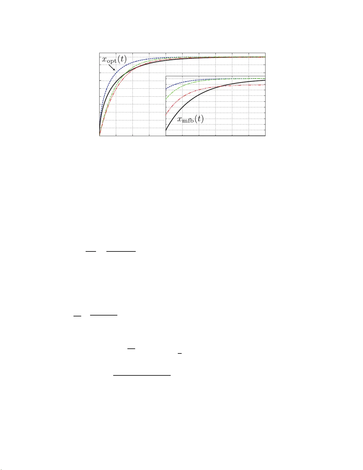
Quan tum feedbac k for rapi d state prep aration in the pres ence of con trol imp erfection s Josh ua Com b es Cent r e for Quantum Computation and Communication T echnology (Australian Research Council), Cen tre for Quantum D yna mics, Griffith University , Brisbane, Queensland 411 1, Australia School of Engineer ing, Australian National University , Can b erra , A CT 020 0 , Australia Cent er for Quantum Information and Control, Univ ersity of New Mexico, Albuquerque, NM 871 31-0 001, USA Ho wa rd M. Wiseman Cent r e for Quantum Computatio n and Communication T echnology (Austra lian Research Council), Cent r e fo r Quantum Dynamics, Griffith University , Brisbane, Queensland 411 1, Austra lia Abstract. Quantum feedback control protoco ls can improv e the oper ation of quantum devices. Here we exa mine the per formance of a purifica tion pr oto col when there are imp erfections in the controls. The ideal feedback protoc o l pro duces an x eigenstate from a mixed state in the minimum time, and is known as rapid state preparatio n. The imp erfections we examine include time delays in the feedback lo op, finite strength f eedba ck, calibra tion error s, and inefficient detec tio n. W e ana ly se these imp erfections us ing the Wiseman-Milburn feedback master equation and re lated formalism. W e find that the proto co l is most sensitive to time delays in the feedba ck lo op. F or systems with slow dynamics, how ever, our analys is sugg e s ts that inefficient detection would b e the bigge r problem. W e also show how system imperfectio ns, such as dephasing and damping, can be included in mo del via the feedback master equation. P ACS num b ers: 03.67.a , 02 .30.Yy , 02.50.r, 89.70.a Keywor ds : quan tum feedbac k, quan tum con trol, imp erfections, rapid state preparation, purification Quantum fe e db ack f o r r apid state pr ep ar a tion in the pr es e n c e of c ontr ol imp erfe ctions 2 1. Motiv ation It is w ell kno wn that imp erfections in feedbac k con trol proto cols— suc h as finite strength feedbac k, inefficien t detection, and lo op dela ys — sev erely degra de the con trollability of some systems [1 , 2, 3, 4]. In this pap er w e are in terested in these types of control imp erfections, as w ell as imp erfect op erations and non-negligible damping. In the in terest of k eeping this analysis manageable w e restrict ourselv es to a single, v ery simple measuremen t model, whic h w e no w describ e. Measuremen t-based quan tum feedbac k proto cols often consider a system (we will examine a qbit) that has an interaction with a prob e (a curren t or field) that results in a con tin uous quan tum non-demolition (QND) [4 ] meas uremen t ‡ of the system. The c hange to the system state ρ during con tin uous measurem ent of a n observ able X is dρ = dt L c [ X ] ρ ≡ 2 γ d t D [ X ] ρ + p 2 γ η dW ( t ) H [ X ] ρ. (1) The first term, D [ A ] ρ ≡ AρA † − 1 2 ( A † Aρ + ρA † A ), describ es the measuremen t bac k action on the state. The final term, H [ A ] ρ ≡ Aρ + ρA † − T r  ( A † + A ) ρ  ρ , represen ts the refinemen t to the observ er’s state of kno wledge due to the measurem ent process [6, 4]. The p ositiv e co efficien t η is the measuremen t efficiency . An efficien t measuremen t corresp onds to η = 1 , while an inefficien t measuremen t corresp onds to η < 1. The measuremen t result in the interv al [ t, t + dt ) is d R ( t ) = √ 4 γ dt h X i + dW ( t ) / √ η , where dW ( t ) is the Wiener pro cess a pp earing in Eq. (1) [7]. The inte gra ted curren t is giv en b y R ( t ) = R t 0 dR ( s ). In this situation the most general feedbac k strategy consists of a pplying a conditional Hamiltonian (which ma y b e a functional of the en tire record up to tha t time) to the system to effect the desired o utcome. An imp orta nt class of feedbac k strategies are those where the f unctional of the record is also a function of t he b est estimate of the system state. These strategies are called Bay esian [8] or state-based feedbac k [9]. In general, implemen ting feedbac k inv olv es engineering driv en Hamiltonian terms of the form P k − idtα k ( t )[ H k , ρ ] to Eq. (1). It is common to a ssume that the controls a v ailable are sufficien tly strong and fast that one ma y consider directly con trolling the state or measuremen t basis through a unitary U . (Note that this do es not break a n y rotating w a ve approximations as w e only require | α | ≫ | γ | .) In this case the conditional state after the measuremen t and feedbac k is ρ ( t + dt ) = ρ + dt L c  ˇ X  ρ in the Heisen b erg picture with res p ect to the con trol unitary , where ˇ X = U † ( t ) X U ( t ). Another imp or t an t class of feedbac k control strategies can b e describ ed b y the Wiseman-Milburn Marko vian feedbac k master equation (FBME) [1 0, 11, 4 ]: ˙ ρ = L [ ρ ] ≡ − i ~  ~ √ 2 γ 2 ( X F + F X ) , ρ  + 2 γ D  X − iF √ 2 γ  ρ ‡ A simplified definition o f a QND measurement is one wher e the measured obser v able commutes with the time evolution o pe rator of the combined pr ob e field and sys tem, i.e. [ U, X ] = 0 . See Refs. [4, 5] for a tho ug h treatment. Here we do not consider the control unitary to b e included in this U — its action (after the mea surement) certa inly do es not commute with X , as we will see. Quantum fe e db ack f o r r apid state pr ep ar a tion in the pr es e n c e of c ontr ol imp erfe ctions 3 + 1 − η η D [ F ] ρ. (2) This can b e deriv ed b y considering instan taneous feedbac k of the current via the feedbac k Hamiltonian H fb ( t ) = F dR ( t ) /d t , and a v eraging ov er the measuremen t noise to obtain a deterministic equation [1 1, 4]. Here F is a Hermitian o p erator, heuristically c hosen to effect the desired outcome. Mark o vian feedbac k is not as p o we rful as Bay esian feedbac k; it do es how ev er ha ve the adv an tage that it is exp erimentally and theoretically simpler. In this ar t icle w e systematically examine the effect of imp erfections in quantum feedbac k pro to cols with a sp ecific example – rapid state preparation (which is v ery closely related to Ja cobs’ rapid purification of a qbit [12, 13, 14]). W e ha v e c hosen this proto col for a n um b er of reasons. Firstly , rapid state preparation (RSP) has a ll of the ingredien ts of more complicated con trol pro t o cols and exp erience sho ws that analysis of RSP often admits analytical solutions. Secondly RSP , as w e shall so on see, is a highly quan tum proto col as it requires con tin ually creating (or stabilizing) a state that is a sup erp osition of the p ointer b asis [15] — what w ould, for a larger system, b e called a Schr¨ odinger cat state. Consequen tly studying the effects of imp erfections on quantum control prot o cols will help delineating in what regimes control will b e of practical imp orta nce. Finally , m uc h of the excitemen t ab out quan tum information theory stems from the sp eed-ups ov er classical proto cols. The RSP pro t o col is one quan tum con trol proto col that offers suc h a speed-up. In the ideal limit, the RSP proto col can b e ac hiev ed with Marko vian feedbac k. T o main tain analytic results, in this article w e w ork within the framew ork of Marko vian feedbac k; if w e had work ed in the Bay esian feedbac k fr a mew ork we w ould ha v e b een forced to rely on nume rics to o btain any results. There is also the p ossibilit y of using risk sensitiv e or r o bust quan tum con trol [16] to examine the problems, but suc h analysis is also likely to b e more complicated than the analysis we presen t. This ar ticle is organized as follo ws. In Sec. 2 w e presen t a proto col f or state preparation that minimises the use of feedbac k control to the application o f one conditional unitary . In Sec. 3 we presen t t he general theory for RSP allow ing fo r con tin uous mo dulation of a feedback Hamiltonian under ideal conditions. Then eac h of these imp erfections described ab o ve are examined in turn in Sec. 4. Finally w e conclude b y comparing the relativ e detrimental effects of each imp erfection. 2. State preparation with one conditional unitary W e b egin b y presen ting the simplest state preparation prot o col for pro ducing a qbit in an x eigenstate, based on con tinuous monitoring of the z comp onent of a ngular momen tum i.e. J z . (W e c ho o se to use J z rather tha n the P auli op erators as it will make comparing our results to other results in t he literature easy . This is b ecause m uc h of the w ork in the literature is for qudits.) It is o bvious that this measuremen t in isola t ion will only pro duce eigens tat es of J z . Th us, to pro duce an x eigenstate at time t f w e a ssume that Quantum fe e db ack f o r r apid state pr ep ar a tion in the pr es e n c e of c ontr ol imp erfe ctions 4 it is p ossible to p erform an instantaneous conditional unita ry at that time to rotate the Blo c h vec tor to the desired x eigenstate. This is the obvious metho d for minimising the use of feedback con trol. W e a ssume here (and in all subseq uent prot o cols) that initia lly the qbit is in a completely mixed state. W e quantify the effectiv eness of this proto col b y the probabilit y that it w ould b e v erified (b y a hypothetical pro j ective measuremen t) to hav e pro duced an x -eigenstate at time t f , as motiv ated in Ref. [14 ]. This probability is linear in the x comp onen t of the Blo ch vector after the final conditional unitary rotat io n. This in turn is equal to the length of the Blo c h v ector prior to that rotation. W e tak e this av erage length as the figure-of-merit for a ll of our proto cols. In the presen t case, it is p ossible to obt a in a closed form expression for the av erage Blo c h v ector length a s a function of the measuremen t record b y using linear tra jectory theory [17, 18, 1 9 ]. This inv olv es using a linear, and necessarily unnorma lized, vers ion of Eq. (1), called t he linear SME d ¯ ρ = dt ¯ L c [ J z ] ρ = 2 γ dt D [ J z ] ρ + p 2 γ dR ¯ H [ J z ] ρ, (3) where ¯ H [ A ] ρ = Aρ + ρA † . Here t he bar denotes the lack of no rmalization. Giv en that ρ (0) and our observ able J z comm ute, t he solution to the SME is [6] ¯ ρ ( R, t ) = exp( − 4 γ J 2 z t ) exp(2 p 2 γ J z R ( t )) I / 2 , (4) where R ( t ) is the integrated photo curren t. Omitting the time dep endence on R for compactness, the solution for a qbit can be exp ressed as ¯ ρ ( R, t ) = e − γ t 2 e √ 2 γ R 0 0 e − √ 2 γ R ! . (5) The norm of Eq. (4) is N = T r [ ¯ ρ ( R , t )] = e − γ t cosh ( √ 2 γ R ). The normalised state is then ρ ( R, t ) = ¯ ρ ( R, t ) / N . The actual probabilit y densit y for the result R is P ( R, t ) = T r [ ¯ ρ ( R, t )] P ( R, t ). Here P ( R, t ) = e − R 2 / (2 t ) √ 2 π t (6) has b een called the ostensible probability for the result R [18]. The ostensible probability is the probability with whic h the record R should b e generated if Eq. (3) w ere to b e used in pla ce of t he normalized SME (1). With these results w e may no w calculate the av erage Blo ch v ector length. F irst w e note tha t the Blo ch v ector length is g iven b y 2 λ max [ ρ ] − 1, where λ max [ ρ ] is the larger eigenv alue of the normalized state ρ . F rom Eq. (5), this will corresp ond to the probabilit y of b eing in the + z eigenstate or the − z eigenstate, dep ending on whether R is p ositiv e or negativ e. Using the symmetry of P ( R ) a nd Eq. (5) the maxim um eigen v alue is h λ max ( t ) i = 2 Z ∞ 0 λ max [ ρ ( t )] N ( R ) P ( R ) dR = 1 √ 2 π t Z ∞ 0 e − ( R − √ 2 γ t ) 2 / 2 t dR Quantum fe e db ack f o r r apid state pr ep ar a tion in the pr es e n c e of c ontr ol imp erfe ctions 5 = 1 2 [1 + erf ( √ γ t )] . (7) When t ≫ γ − 1 (the long-time limit) this express ion can b e approx imated b y h λ max ( t ) i L T = 1 − 1 2 e − γ t √ π γ t , (8) where the subscript L T denotes that this expression is only v alid in the long-time limit. W e can relate this express ion to h x mfb i , t he mean length of the Blo ch vec tor (or its x -comp onen t after the final r otation) by h x mfb ( t ) i = 2 h λ max ( t ) i − 1 . (9) Here the subscript ‘mfb’ signifies that this proto col minimises the use of feedbac k con trol. W e a lso refer t o this as the op en-lo o p strategy b ecause the conditio nal unitary happ ens after all measuremen ts so it is feedforward. 3. Ideal rapid state preparation Consider aga in a qbit in whic h J z is contin uously monitored but now w e assume that for arbitrarily strong feedbac k-induced rotatio n around the y axis is av ailable. This is all that is required for con trol given that the measured observ able pic ks out the z axis, and that the aim is to maximize h x ( t f ) i . As w e will see, the optimal feedbac k proto col in this situation is of the f orm described b y Eq. (2 ) , where H fb ( t ) dt = F dR ( t ), prov ided F ( t ) itself is allow ed to b e time dep enden t: F ( t ) = Ω( t ) J y . Equation (2) will th us pro vide the ba sis for the fo llowing study . Giv en the ab o v e senario and allo wing for a time dep enden t feedbac k strength, Ω( t ), and assuming efficien t measuremen ts ( η = 1), equation 2 b ecomes ˙ ρ = 2 γ D  J z − i Ω( t ) J y √ 2 γ  ρ. (10) F rom Eq. (10) w e may find the the equations of mot io n f o r the Blo ch comp onen ts. This is ac hiev ed b y taking the trace of Eq. (10) with the comp onent of in terest, for example ˙ x = T r [ σ x ˙ ρ ]. The r esulting equations are ˙ x = − xγ − Ω( t ) 2 2 x + p 2 γ Ω( t ) (11) ˙ y = − γ y (12) ˙ z = − Ω( t ) 2 2 z (13) By solving d Ω ˙ x = 0 for Ω, where d Ω ≡ d/d Ω, the feedbac k whic h lo cally mazimizes the rate at which the ˙ x comp onen t gro ws can b e found. This giv es the optimal feedbac k strength as a function of x : Ω opt ( x ) = √ 2 γ /x . Using this and the init ia l condition x (0) = 0 the solution to Eq. (11) is x opt ( t ) = √ 1 − e − 2 γ t . (14) Quantum fe e db ack f o r r apid state pr ep ar a tion in the pr es e n c e of c ontr ol imp erfe ctions 6 The optimal feedbac k strength as a function of time is computed by substituting Eq. (14) in to Ω opt : Ω opt ( t ) = √ 2 γ √ 1 − e − 2 γ t . (15) This is precisely the ev olution of Jacobs’ rapid purification proto col giv es [12]. Moreov er, Wiseman a nd Bouten ha v e sho wn that this is the g lobally optimal control proto col for this problem [14] (see also Ref. [2 0 ]). T o calculate the impro ve ment feedback offers w e solv e x mfb ( t mfb ) = x opt ( t opt ) for the ratio of t opt /t mfb . T hen we ta ke the limit tha t t mfb → ∞ to give t opt /t mfb = 1 /S = 1 / 2. Th us the asymptotic sp eed-up (improv emen t) of the ideal feedbac k ov er the minimal con tro l (op en-lo o p) proto col to pro duce a state with a giv en fixe d v alue of x ( t f ) v ery close to one is S = 2. Of course, once the desired Blo c h v ector length is reached w e ma y rotate final state to any desired state, as w e hav e assumed an effectiv ely instan taneous rotation. Th us we may rapidly prepare any qubit state. 4. Rapid st ate preparation w ith imp erfect ions W e now calculate the effect o f four differen t imp erfections or limitations o n the ra pid preparation of an x eignens tate b y feedbac k. 4.1. Constant fe e db ack str ength First w e conside r the case where the feedbac k strength is t ime indep enden t (constan t). It is unclear whether suc h a strategy can ra pidly purif y at all, a nd, if it can, whether it affo r ds the same a symptotic a dv an tage a s the optimal strategy . In addition this analysis is imp ortan t experimen tally for tw o reasons. Fir stly , a fixed feedbac k strength is simpler to implemen t exp erimentally . Secondly , the optimal feedbac k strength ( 1 5) is un b ounded at time zero, so with the ana lysis here w e can prob e the usefulnes s of b ounded strength con trols. Based on the asymptotic v alue of the o ptimal feedback strength Ω opt ( ∞ ) = √ 2 γ , w e parameterize the constan t f eedback strength as Ω = √ 2 γ α , where α ∈ ( −∞ , ∞ ). The x Blo ch comp onen t becomes ˙ x = − xγ − Ω 2 2 x + p 2 γ Ω = − xγ − γ α 2 x + 2 γ α . (16) Solving this equation with the initial condition x (0) = 0 gives x ( t ) = 2 α 1 + α 2 (1 − e − γ t (1+ α 2 ) ) . (17) In F ig. 1, Eq. (1 7) is plotted for differen t v alues of α . Negativ e v alues of α r esult in the − x eigenstate being prepared. When | α | > 1 the x comp o nent of the Bloch v ector rapidly increases for t ≪ γ − 1 but reaches a steady state v a lue less than one. When Quantum fe e db ack f o r r apid state pr ep ar a tion in the pr es e n c e of c ontr ol imp erfe ctions 7 | α | < 1 the Blo ch ve ctor increases mor e slow ly , and also asymptotes to a v alue less than one. 0.1 0.2 0.3 0.4 0.5 0.6 0.7 0.8 0.9 1 Bloch vector length 0 0.2 0.4 0.6 0.8 1 1. 2 1. 4 1. 6 1. 8 2 Ti m e ( γ -1) Figure 1. The x co mp o nent of the Blo ch vector for differen t constant feedback strategies. The do tted line (blue) is the ideal feedback i.e. Eq. (14). The thic k solid line (black) is for the op en-lo o p control pro to col, i.e. Eq. (7). The re ma ining lines ar e for the consta nt feedback str e ngth strategies. The feedback streng th is para meterized by Ω = √ 2 γ α wher e α ∈ ( −∞ , ∞ ). F r om the upp ermost curve the solid lines (green) are for α = 1 , 3 , 5 and 1 5. T he das hed lines (green), sta rting from the upper most curve, are for α = 0 . 5 , 0 . 25 , 0 . 1 a nd 0.02 5. The steady state at long- times is x ss = 2 α (1 + α 2 ) − 1 , whic h is maximized for α = 1, in whic h case x ( t ) = 1 − e − 2 γ t . (18) In F ig . 1 w e analyse the short to medium time regime. The optimal constan t feedbac k b egins to out-p erform the no feedbac k case for t > 0 . 768 γ − 1 . Figure 2 shows the long time regime, in whic h it is app ears that Eq . (18) approac hes the the optimal time dep enden t feedbac k curve (14). Intere stingly , when α = 0 . 9 the feedbac k p erforms w orse than the op en-lo op con trol until t > 1 . 53 γ − 1 . F o r 1 . 53 γ − 1 < t < 3 . 6 5 γ − 1 feedbac k p erforms b etter, a nd after this in terv al the feedback again p erfor ms worse than the op en- lo op con trol. This suggests that an optimal state preparation (or purificatio n) proto col for b ounded strength control (or bang-bang control) migh t switc h b et we en p erio ds of feedbac k and measureme nt multiple times. The only question that remains is whether the optimal constan t feedbac k strength proto col ha s the same asymptotic adv an tage as the optimal time dep enden t f eedback . This can b e determined b y comparing the ratio of the t ime tak en to a fixed Blo c h v ector length 1 − ǫ . T a ylor- expanding Eq. (14) at long-times giv es x opt ( t ) = 1 − 1 2 e − 2 γ t opt . Setting this equal to 1 − ǫ and solving for t opt giv es the time taken to a fixed Blo ch v ector length. Quantum fe e db ack f o r r apid state pr ep ar a tion in the pr es e n c e of c ontr ol imp erfe ctions 8 0 0.2 0.4 0.6 0.8 1 0 0.5 1 1.5 2 2.5 3 3.5 4 4.5 5 0.96 0.97 0.98 0.99 1 Ti m e ( γ -1) Bloch vector length Figure 2. A compa rison of the time it takes to prepar e an x eigenstate for four different strategies. The dotted line (blue) is fo r the o ptimal time dep endent feedback – that is, Eq. (14). T he thick line (black) is the Blo ch vector length for the op en-lo o p control proto col. The dot-dash (gr een) line is the asymp ototicly optimal co nstant feedback ( α = 1), Eq. (1 8). The dot-dot-das h (red) line is sub-optimal constant feedba ck – that is, Eq. (17) with α = 0 . 9. Inset: an ex plo ded version of the same plot. This pro cess must b e r ep eated for Eq. (18) ; the time at whic h Eq. ( 1 8) reac hes 1 − ǫ is denoted by t c . The ratio of the t imes is t c t opt = ln ǫ ln ǫ + ln 2 (19) whic h a ppro ac hes 1 as ǫ approac hes zero. 4.2. Calibr ation err ors Consider now the case in whic h the applied control has calibration errors. F or the optimal time-dep enden t control a time-dependent calibration error could b e mo delled b y Ω( t ) = ( √ 2 γ / √ 1 − e − 2 γ t )(1 + δ ), where δ ∈ [ − 1 , 1]. Because these errors a re systematic it is sensible to assume that δ is constan t. Substituting Ω( t ) into the Blo ch equations giv es ˙ x = − γ x + p 2 γ Ω( t )(1 + δ ) − 1 2 Ω( t ) 2 (1 + δ ) 2 x. (20) This has the solution x ( t ) = p (1 − e − 2 tγ ) (1 − δ 2 ) . (21) A t long-times this asymptotes t o x ss ∼ 1 − δ 2 / 2 for small δ . In Fig. 3 we plot Eq. (21) for differen t calibrat io n error v alues . A 25% calibration error p erforms w orse than the op en- lo op proto col for t > 2 . 15 γ − 1 . How ev er, provided the calibration error is less than 5% feedbac k control will out- p erform op en-lo op con trol for t ≤ 5. F or comparison w e also plot the p erformance of the asymptotically optimal constant feedbac k proto col, whic h outp erforms the time-dep enden t feedbac k with a 5 % calibration error for t ≥ 3 . 05 γ − 1 . Quantum fe e db ack f o r r apid state pr ep ar a tion in the pr es e n c e of c ontr ol imp erfe ctions 9 10 −3 10 −2 10 −1 5 0 0.2 0.4 0.6 0.8 1 Ti m e ( γ -1) 1 3 4 5 0.99 0.995 1 Bloch vector length Figure 3. The effect of time-dep endent calibratio n errors on RSP . As befo r e the dotted line (blue) is the optimal control; the dot-das he d line (green) is the o ptimal constant ( α = 1) control; and the thick line (black) is the op en-lo o p co ntrol str ategy . The three dashed (magenta) lines from top to bo ttom are for δ = [0 . 25 , 0 . 5 , 0 . 75]. The dashed line on the inset figure depicts δ = 0 . 05. 4.3. Efficienc y and noise on c ontr ol err ors No w consider the case in whic h the exp erimen t is constrained by a detection inefficiency η . W e analyse this scenario in t w o wa ys. First w e examine the situatio n when the exp erimenter applies the con trol una w are of detection inefficienc ies. The second scenario is more realistic. Here w e assume that there is a detection inefficiency and ask what the optimal control in this situation is. Note tha t detection inefficiency also describ es the case when there is r andom noise on the con trol [4]. W e note that the effect of detection inefficiency on a related rapid purification proto col w as studie d in Ref. [21]. 4.3.1. Oblivious ineffici e nt dete ction When the system is constrained by inefficien t detection the eq uatio n of motion for the x Blo c h comp onent is ˙ x = − xγ + √ 2 √ γ Ω − x Ω 2 2 η . (22) If one we re oblivious to the detection inefficiency , one would apply the optimal con trol, Ω opt ( t ), from Sec. 3. The solution of the equation o f motio n under suc h a con trol strategy is x ( t ) = r 2 η − 1 η √ 1 − e − 2 γ t . (23) Clearly the protocol only w orks f o r η ∈ (0 . 5 , 1] a nd asymptotically the greates t ac hiev able Blo ch vec tor length is x ss = √ 2 η − 1 / √ η . 4.3.2. Optimal c ontr ol for ineffici e n t dete ction T o optimize the control for inefficien t detection one simply tak es the deriv ativ e o f Eq. (22) with resp ect to Ω a nd solv es to Quantum fe e db a ck for r apid state p r ep ar ation in the pr esenc e of c ontr ol imp erfe ctions 10 find the optimal con trol Ω η ( t ) = √ 2 γ η x . (24) The solution of the x comp onen t using this strategy is x ( t ) = √ η p (1 − e − 2 tγ ) . (25) Asymptotically the steady state v alue of this stratergy is x ss = √ η . In F ig. 4 the steady state v alues of Eq. (23) and Eq. (25), are plotted fo r all v alues of η . The control o ptimized for detection inefficiencies, Eq. (25), ob viously outp erforms the oblivious con trol case for all η . This is eviden t in Fig. 5, where Eq. (2 3) and Eq. (25) a re plotted for η = 0 . 85 , although the t w o strategies are barely distinguishable. With this efficiency , the stat e preparation b ecomes w orse than that o f constant feedbac k strength, and that of the op en-lo op strategy , for t & γ − 1 . 0 0.1 0.2 0.3 0.4 0.5 0.6 0.7 0.8 0.9 1 0 0.2 0.4 0.6 0.8 1 η (dimensionless) Steady State Bloch vector length Figure 4. A compa rison of the stea dy state inefficiencies fo r the oblivious control scheme, plo tted as the solid line (r e d), and the optimal co ntrol for inefficient detection dotted line (blue). 4.4. Time delay While Eq. (2) is a very general FBME, it assumes instan taneous feedbac k (that is, zero dela y time in the f eedbac k lo op). It is p ossible to include the effects of a small finite time delay in the analysis while still using a master equation approac h [22]. Note ho w ev er that the resulting equation is not guaran teed to b e a v alid (Lindblad-f o rm) master equation a nd will a lmost certainly give nonphy sical results for τ to o large with resp ect to γ − 1 . The equation describing the feedbac k pro cess including a small time dela y τ is [2 2] ˙ ρ = L [ ρ ] − iτ p 2 γ [ F , L [ X ρ + ρX ] − X ( L [ ρ ]) − ( L [ ρ ]) X ] . (26) Recall that L [ . ] was defined in Eq. (2 ). Substituting X = J z and F = Ω( t ) J y in to Eq. (26), and setting η = 1 giv es ˙ ρ = L [ ρ ] − iτ Ω( t ) p 2 γ [ J y , L [ J z ρ + ρJ z ] − J z ( L [ ρ ]) − ( L [ ρ ]) J z ] . (27) Quantum fe e db a ck for r apid state p r ep ar ation in the pr esenc e of c ontr ol imp erfe ctions 11 10 −3 10 −2 10 −1 0 0.2 0.4 0.6 0.8 1 Ti m e ( γ -1) 1 5 Bloch vector length Figure 5. A compariso n of the dynamics of the x comp onent of the Blo ch vector at relatively short times for the oblivio us control scheme (the low er dot-dot-dashed line) and the optimal co ntrol for inefficient detection (the das hed line); η = 0 . 85 . The dotted line is the optimal control; the dot-dashed line is the optimal cons tant ( α = 1) control; and the thick line is the op en-lo op co ntrol strategy . F rom this equation it is straight-forw ard to calculate the dynamical equations for the Blo c h components: ˙ x = − xγ + p 2 γ Ω − x Ω 2 2 − √ 2 γ Ω 3 τ 2 (28) ˙ y = − γ y (29) ˙ z = − z Ω 2 2 − 2 z Ω 2 γ τ . (30) The feedbac k strength, Ω, mu st no w b e c hosen in order to rapidly prepare an x eigenstate. As for t he case of inefficiencie s, w e choo se tw o scenarios to prob e time delays in RSP . The first scenario, presen ted in Sec. 4.4.1, ex amines the p erformance o f a control proto col which has time dela ys, but the exp erimen talist is oblivious to these delays . The second situatio n the exp erimentalist is aw are of the feedbac k delay and comp ensates for it, whic h is presen ted in Sec. 4.4 .2. In b oth cases we tak e the feedbac k strength Ω to b e constant, equal to its asymptotically optimal v alue. This is necessary t o o bta in analytical results, as o btained in a ll of the other sce nario s in this pap er. 4.4.1. Oblivious time de lay Consider an exp erimentalist who is una w are of time delay s in their feedback lo op. Due to the cost and difficulties of applying time dep enden t con trols the exp erimen talist decides to apply asymptotically optimal time independent con trol Ω = √ 2 γ in their RSP pro cedure. The solution o f Eq. (28) in this scenario is x ( t ) =  1 − e − 2 tγ  (1 − γ τ ) . (31) The steady state solution is x ss = 1 − γ τ . In Fig. 6 Eq. (31) is plott ed for differen t time dela ys. Quantum fe e db a ck for r apid state p r ep ar ation in the pr esenc e of c ontr ol imp erfe ctions 12 Asymp. opt. control for time delays Oblivious 10 −1 Ti m e ( γ -1 ) 1 5 0 0.2 0.4 0.6 0.8 1 Bloch vector length Figure 6. A comparis on o f different feedback str ategies for different time delays. The dotted line is the o ptima l control; the dot-dash line is the optimal constant ( α = 1) c ontrol; and the think line is the meas urement a lone s trategy . The dashed lines (mage nta) from top to b ottom are for feedback with oblivious time delay with τ = 5 × 10 − 2 γ − 1 , 10 − 1 γ − 1 . The dot-dot-das hed lines (cyan) from top to b ottom are for the asy mptotically optimal control with time delays τ = 5 × 10 − 2 γ − 1 , 10 − 1 γ − 1 . 4.4.2. Asymptotic al ly optimal c ontr o l fo r time delays Consider first a lo cal-in-time optimization of Eq. (28). This is again ac hiev ed b y solving d Ω ˙ x = 0 for Ω, whic h give s Ω ± opt = − x ± p x 2 + 12 γ η τ / (3 √ 2 γ τ ). A second deriv ativ e test sho ws that Ω + opt is the lo cal maxim um, th us w e define Ω opt ≡ Ω + opt . As Eq. (26) is a p erturtabative correction to order τ , it is only sensible to consider the terms to order τ : Ω opt = √ 2 γ η x − 3 √ 2 γ η 2 γ τ x 3 + O ( τ 2 ) . (32) If w e restrict, as in the oblivious case, to cons tant fe edback , § then optimal asymptotic v alue in the presence of time delays is thus Ω = √ 2 γ (1 − 3 γ τ ). Under this con trol statergy the solution o f ˙ x is x ( t ) = 2(1 − 3 γ τ ) 2(1 − 3 γ τ ) + 9 γ 2 τ 2  1 − e − 2 γ t +6 γ 2 τ t − 9 γ 3 τ 2 t  (33) It is apparent from Fig. 6 that the asymptotically opt imal control significan tly outp erforms the oblivious senerio for t & γ − 1 . In fact it gives a final Blo c h vec tor length of almost unity . This is b ecause the co efficien t Eq. ( 3 3), to first order in τ , is unit y . Ho w ev er the terms in the exp o nen t slo w t he purification, so that no improv eme nt o v er the op en-lo op case is found at any t ime ev en for τ = 0 . 0 5 γ − 1 . 5. Comparison of imp erfections In order to compare the imp erfections w e determine the allow ed parameter r anges for the different imp erfections that will enable the feedbac k con trol case to p erform b etter § The alternative would b e to so lve the problem numerically . The rele v ant equation with lo cally optimal feedback ( 32 ) is ˙ x = − xγ + γ η /x − 2 γ 2 η 2 τ / x 3 . Quantum fe e db a ck for r apid state p r ep ar ation in the pr esenc e of c ontr ol imp erfe ctions 13 than the minimal con trol ( o p en-lo op) pro to col at t = 2 γ − 1 and t = 4 γ − 1 . Althoug h the c hoice of times is arbitrary , the first time chos en is, r oughly , when the long-time limit ( t ≫ γ − 1 ) appro ximation b egins to b e reasonable, while t he second is w ell in the asymptotic regime. T able 1 summarizes the results. Con trol Imp er fection P arameter Range A Parameter Range B Constan t FB strength 0 . 956 ≤ α ≤ 1 . 189 0 . 9415 ≤ α ≤ 1 . 0 678 Time dep. cal. errors 0 ≤ δ ≤ 0 . 1 65 0 ≤ δ ≤ 0 . 0 659 Inefficien t det. oblivious FB 0 . 973 ≤ η ≤ 1 0 . 9956 ≤ η ≤ 1 Inefficien t det. optimal FB 0 . 972 ≤ η ≤ 1 0 . 9956 ≤ η ≤ 1 Time delay ( γ − 1 ) oblivious FB 0 ≤ τ ≤ 0 . 0045 0 ≤ τ ≤ 0 . 0020 Time delay ( γ − 1 ) optimal FB 0 ≤ τ ≤ 0 . 0146 0 ≤ τ ≤ 0 . 0195 T able 1. The parameter rang es for whic h imp erfect feedba ck per forms b e tter than the minimal control pro to col at a fixed time. The firs t co lumn describ es the type of control imper fection. The second column, Parameter Range A, gives the approximate v alues for the parameter (imp erfection) under considera tion a t t = 2 γ − 1 . The third column, Parameter Rang e B, gives the a pproximate v alues fo r the parameter (imp erfection) under considera tion a t t = 4 γ − 1 . Con trol Imp erfection P arameter Range A Parameter Range B Constan t FB strength 0 . 922 ≤ α ≤ 1 . 135 0 . 9860 ≤ α ≤ 1 . 0 141 Time dep. cal. errors 0 ≤ δ ≤ 0 . 1246 0 ≤ δ ≤ 0 . 0 1412 Inefficien t det. oblivious FB 0 . 9846 ≤ η ≤ 1 0 . 9998 ≤ η ≤ 1 Inefficien t det. optimal FB 0 . 9844 ≤ η ≤ 1 0 . 9998 ≤ η ≤ 1 Time delay ( γ − 1 ) oblivious FB 0 ≤ τ ≤ 0 . 00547 0 ≤ τ ≤ 0 . 0000 996 Time delay ( γ − 1 ) optimal FB 0 ≤ τ ≤ 0 . 02598 0 ≤ τ ≤ 0 . 0046 12 T able 2. The parameter rang es for whic h imp erfect feedback per forms better than the minimal control proto col at a fixed Blo ch vector length. The first column describ es the type of control imp erfection. The second column, Parameter Ra ng e A, gives the approximate v alues for the parameter (imp erfection) under c o nsideration at x = 1 − 10 − 2 . The third co lumn, Parameter Range B, gives the appr oximate v alues for the par ameter (imperfectio n) under co nsideration at x = 1 − 10 − 4 . F rom Fig. 1 it w as clear that α ≫ 1 is required for short time ev olution to p erform lik e the op en-lo op ev olution, but the dynamics induced b y a large α caused the steady state Blo ch v ector length to b e po or. Th us t he second row in T able 1 suggests that strong feedbac k is not necessary a s α is of order 1. This implies tha t b ounded strength con trol prot o cols can w ork in RSP . The third ro w in T able (1 ) suggests that the feedbac k proto col is not v ery sensitiv e to calibration errors, as a 16 . 5% error in the calibration seems rather high. Quantum fe e db a ck for r apid state p r ep ar ation in the pr esenc e of c ontr ol imp erfe ctions 14 The fourth and fifth rows of T able 1 show the effect of detection inefficiencies on RSP . Ev en in quan tum optics with high-efficiency homo dyne detectors, the ov erall efficiency is seldom greater than η < 0 . 9 (see e.g. R ef. [23]). Thus , unfortunately , the RSP proto col is lik ely to b e sev erely compromised by detection inefficiencies, regardless of whether one is a w are of them or not. These ro ws also represen t the effects of white noise on the con trol. The final ro w indicates that RSP is most sensitiv e to time dela ys. Outside the small τ regime it is unlik ely that this sort of RSP will b e feasible using Mark ovian or Ba y esian f eedback . k If, how ev er, a par t icular ph ysical system has γ − 1 whic h is of the order o f a Meghertz (o r smaller) t hen feedbac k dela ys due to classical circuitry could b e made m uc h smaller than γ − 1 . In this case RSP is r emark ably ro bust to time delay s, in the sense that the asymptotic x ss differs from unity only in second order in the dela y τ . In T able 2 w e consider the parameter rang es tha t allow feedbac k to p erform b etter than the minimal con trol proto col at a fixed Blo c h v ector length. W e consider t wo lengths: x = 1 − 10 − 2 (the second column) and x = 1 − 1 0 − 4 (the third column). The same trends describ ed ab o ve also hold for this table. 6. Discussion The most imp o r tan t conclusion of our a na lysis is tha t quan tum feedback control for rapid state preparation is quite sensitiv e to detection inefficiencies. In particular, lo cally optimizing the feedbac k, taking into accoun t the efficiency η , limits the length of the Blo c h vec tor in the long-time limit to √ η . How ev er, our analysis also turned up some encouraging conclusions. Surprisingly , con trol in an un biased basis seems ro bust to dela ys in the feedbac k loo p, at least in the sense that the asymptotic Blo c h differs from unit y only in second order in the dela y τ . The metho dology presen ted in this a r t icle, a pproximating Ba y esian feedbac k with Mark o vian feedbac k, is not restricted to studying imp erfections in the con trol. It also allo ws one to study the p erformance of control proto cols with system imp erfections. F or example, consider p erforming RSP when the sys tem has isotropic dephasing no ise at rate Γ iso and the deca y rate fr o m the excited state is Γ d . The F BME in this situation is: ˙ ρ = L [ ρ ] + X i ∈ x,y ,z Γ iso D [ σ i ] ρ + Γ d D [ σ − ] ρ. (34) F rom this equation it is easy to deriv e an equation for x ( t ) x ( t ) = r 2 γ η 2 γ + 8Γ iso + Γ d p 1 − e ( − 2 tγ − 8 t Γ iso − Γ d t ) . (35) Here we are mo delling lo cally optimal rapid state prepara tion, with detection inefficiency included as a control imp erfection. The main p oin t is that, b y approximating Bay esian k W e note, how ever, that the op en-lo o p s cheme prese nt ed in Ref. [ 3 ] allows sub-optimal RSP with a single conditional unitar y at the e nd, as in the minimal control pro to col of Sec. 2 . Quantum fe e db a ck for r apid state p r ep ar ation in the pr esenc e of c ontr ol imp erfe ctions 15 feedbac k with Mark ovian feedbac k we can b egin to a na lyse analytic al ly the p erformance of f eedback proto cols with man y different con trol or system imp erfections. W e note that the effect of x dephasing and deca y f rom the excited state w as studied in Ref. [24].The adv an tage of our metho d is tw o fold: firstly our analysis is algebraically simpler; and secondly w e deriv e time-dep enden t solutions, not just steady state v alues. In f ut ure w ork w e think it would also b e interesting to see if the Mark ov ian a pproac h to rapid x -eigenstate preparation presen ted here could be generalized to all qbit states (b y analo gy with the stabilization of a qbit under monitored sp ontaneous emission in Refs. [25, 8]) with and without imp erfections. A cknow le dgements: This res earch w as conducted b y the Australian R esearch Council Cen tre of Excellence for Quan tum Computation and Comm unication T echnology (pro ject n um b er CE11000 1 029). JC also ac kno wledges supp ort from National Science F oundation Gran t No. PHY-0903953 and Office of Nav al Researc h Gran t No. N00014-1 1-1-00 8. References [1] D. W. Berry and H. M. Wiseman, J. Mo d. Optics. 48 , 797 (2001). [2] J. W a ng, H. M. Wise ma n, and G. J . Milburn, Chemical Physics, 268 , 2 21 (2001). [3] J. Co mbes , H. M. Wiseman, A. J. Scott, P hys. Rev. A 8 1 , 0203 01(R) (2 010). [4] H. M. Wise ma n and G. J. Milburn, Quantum Me asur ement and c ontr ol , (CUP , Ca mb r idge, 2010). [5] V.B. Braginsky , and F.Y. Khalili, Q uantum me asur ement ,(Cambridge Universit y P ress, 1995 ). [6] K. Ja cobs and D. Steck, Contemp. Phys. 4 7 , 279 (20 06). [7] K. Ja cobs, Sto chastic Pr o c esses for Physicists (CUP , Cambridge, 2010). [8] How ar d M. Wiseman and Stefano Ma ncini and Jin W a ng, Phys. Rev. A, 66 , 0 1 3807 (2002). [9] Andrew C. Doherty and Kur t Jacobs, Phys. Rev . A, 60 , 2 700 (1999 ). [10] C. M. Cav es and G. J . Milburn, Phys. Rev. A, 36 , 55 43 (1987). [11] H. M. Wiseman and G. J. Milburn, Phys. Rev. Lett., 70 , 548 (1993 ). [12] K . Jacobs, Phys. Rev . A 67 , 030 301(R) (2003). [13] K . Jacobs, Pro c . o f SPIE, 5468 , 35 5 (2004). [14] H. M. Wiseman and L. Bouten, Qua nt um Inf. P ro cess., 7 , 71 (20 08). [15] W. H. Zurek, P hys. Rev. D 24 , 1516 (1981 ); W.H. Zurek, Quantum Decoherence, 1–31, (2007 ). [16] M. R. Ja mes, P hys. Rev. A, 69 , 032108 (2004 ); M. R. James, J. O pt. B: Q uantum Semicla ss. Opt., 7 , 198 (2005 ). [17] Peter Go etsch and Ro b e r t Graham, Phys. Rev. A, 50 , 524 2, (1994). [18] H. M. Wiseman, Quantum Se micla ss. Opt. 8 , 205 (199 6). [19] K . Jacobs and P . L. Knig ht , Phys. Rev. A. 57 , 2301 (199 8). [20] V. P . Belavkin a nd A. Negr etti and K. Mølmer , Phys. Rev. A, 79 , 0221 23 (20 09). [21] A. Chiruvelli and K . J acobs, Phys. Rev. A, 77 , 01 2102 , (2008 ). [22] H. M. Wiseman, Phys. Rev. A 49 , 213 3 (1994). [23] T. A. Wheatley et al. , P hys. Rev. Lett. 104 , 09 3601 (20 10). [24] J . Li and K. Ja cobs, Quantum Inf. C o mput. 9 , 3 95 (2009). [25] Holg er F. Hofmann, G ¨ unter Mahler and O rtwin Hess, Phys. Rev. A, 57 , 487 7 (1998).