Max-Weight Scheduling in Queueing Networks with Heavy-Tailed Traffic

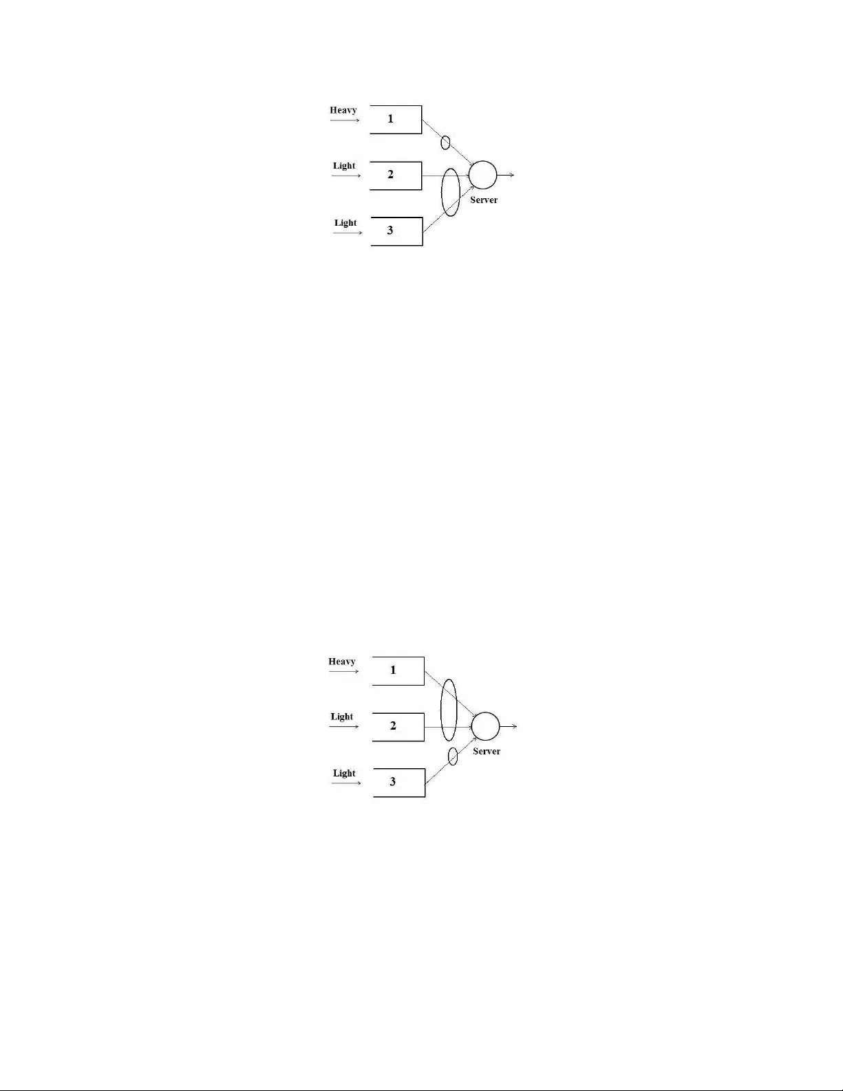
Max-W eigh t Sc heduling in Queueing Net w orks with Hea vy-T ailed T raffic ∗ Mihalis G. Mark akis, Eytan H. Modiano, and John N. Tsitsiklis † Abstract W e consider the problem of pac k et sc heduling in single-hop queueing net w orks, and analyze the impact of hea vy-tailed traffic on the performance of Max-W eight scheduling. As a p erfor- mance metric w e use the dela y stabilit y of traffic flo ws: a traffic flo w is dela y stable if its expected steady-state delay is finite, and delay unstable otherwise. First, we sho w that a heavy-tailed traffic flow is delay unstable under an y scheduling p olicy . Then, we fo cus on the celebrated Max-W eigh t scheduling p olicy , and show that a light-tailed flow that conflicts with a heavy- tailed flow is also dela y unstable. This is true irresp ective of the rate or the tail distribution of the ligh t-tailed flo w, or other scheduling constrain ts in the netw ork. Surprisingly , we sho w that a light-tailed flow can b e dela y unstable, even when it do es not conflict with heavy-tailed traffic. F urthermore, delay stability in this case may dep end on the rate of the light-tailed flow. Finally , w e turn our atten tion to the class of Max-W eigh t- α sc heduling p olicies; w e sho w that if the α -parameters are chosen suitably , then the sum of the α -moments of the steady-state queue lengths is finite. W e provide an explicit upp er b ound for the latter quan tit y , from whic h w e derive results related to the delay stabilit y of traffic flows, and the scaling of moments of steady-state queue lengths with traffic intensit y . ∗ This w ork w as supported b y NSF Gran ts CNS-0915988 and CCF-0728554, and AR O MURI Grant W911NF-08- 1-0238. † The authors are with the Laboratory for Information and Decision Systems, at the Massach usetts Institute of T echnology , Cambridge, MA, USA. 1 1 In tro duction W e study the impact of hea vy-tailed traffic on the p erformance of scheduling p olicies in single- hop queueing net w orks. Single-hop netw ork mo dels hav e b een used extensiv ely to capture the dynamics and scheduling decisions in real-world communication netw orks, such as wireless uplinks and do wnlinks, switches, wireless ad ho c netw orks, sensor netw orks, and call centers. In all these systems, one cannot serve all queues sim ultaneously , e.g., due to wireless interference constrain ts, giving rise to a sc heduling problem. Clearly , the o v erall p erformance of the netw ork dep ends critically on the scheduling p olicy applied. The fo cus of this pap er is on a well-studied class of scheduling p olicies, commonly refered to as Max-W eigh t policies. This class of p olicies was introduced in the seminal work of T assiulas and Ephremides [24], and since then numerous studies hav e analyzed the p erformance of suc h policies in differen t settings, e.g., see [1, 9], and the references therein. A remark able prop ert y of Max- W eight p olicies is their throughput optimalit y , i.e., their ability to stabilize a queueing netw ork whenev er this is p ossible, without an y information on the arriving traffic. Moreo ver, it has b een sho wn that p olicies from this class achiev e low, or even optimal, a verage delay for specific netw ork top ologies, when the arriving traffic is light-tailed [8, 16, 20, 23, 25]. 1 Ho wev er, the p erformance of Max-W eight scheduling in the presence of hea vy-tailed traffic is not w ell understo o d. W e are motiv ated to study netw orks with heavy-tailed traffic b y significant evidence that traffic in real-world comm unication net works exhibits strong correlations and statistical similarit y ov er differen t time scales. This observ ation was first made b y Leland et al. [13] through analysis of Ethernet traffic traces. Subsequen t empirical studies hav e do cumented this phenomenon in other net works, while accompanying theoretical studies hav e associated it with arriv al processes that ha ve hea vy tails; see [17] for an ov erview. The impact of hea vy tails has b een analyzed extensively in the context of single or multi-serv er queues; see the survey pap ers [2, 4], and the references therein. Ho wev er, the related work is rather limited in the context of queueing netw orks, e.g., see the pap er b y Borst et al. [3], which studies the “Generalized Processor Sharing” p olicy . 1 On the other hand, when Max-W eigh t scheduling is combined with Back-Pressure routing in the context of m ulti-hop net works, there is evidence that delay p erformance can b e po or, e.g., see the discussion in [5]. 2 This pap er aims to fill a gap in the literature, b y analyzing the impact of hea vy-tailed traffic on the p erformance of Max-W eigh t sc heduling in single-hop queueing netw orks. In particular, we study the delay stabilit y of traffic flo ws: a traffic flo w is delay stable if its exp ected steady-state dela y is finite, and delay unstable otherwise. Our previous work [15] gives some preliminary results in this direction, in a simple system with tw o parallel queues and a single server. The main con tributions of this pap er include: i) in a single-hop queueing netw ork under the Max-W eigh t sc heduling p olicy , we show that any light-tailed flow that conflicts with a heavy-tailed flow is delay unstable; ii) surprisingly , w e also sho w that for certain admissible arriv al rates, a light-tailed flow can b e delay unstable even if it do es not conflict with heavy-tailed traffic; iii) we analyze the Max- W eight- α sc heduling p olicy , and show that if the α -parameters are chosen suitably , then the sum of the α -moments of the steady-state queue lengths is finite. W e use this result to prov e that by prop er c hoice of the α -parameters, all light-tailed flo ws are delay stable. Moreov er, w e sho w that Max-W eight- α ac hieves the optimal scaling of higher momen ts of steady-state queue lengths with traffic intensit y . The rest of the pap er is organized as follo ws. Section 2 contains a detailed presen tation of the mo del that w e analyze, namely , a single-hop queueing netw ork. It also defines formally the notions of hea vy-tailed and ligh t-tailed traffic, and of dela y stability . In Section 3 we motiv ate the subsequen t developmen t b y presen ting, informally and through simple examples, the main results of the pap er. In Section 4 we analyze the p erformance of the celebrated Max-W eight scheduling p olicy . Our general results are accompanied by examples, whic h illustrate their implications in practical net work settings. Section 5 contains the analysis of the parameterized Max-W eight- α sc heduling p olicy , and the p erformance that it achiev es in terms of delay stabilit y . This section also includes results ab out the scaling of momen ts of steady-state queue lengths with the traffic in tensity and the size of the netw ork, accompanied b y several examples. W e conclude with a discussion of our findings and future research directions in Section 6. The app endices con tain some bac kground material and most of the pro ofs of our results. 3 2 Mo del and Problem F orm ulation W e start with a detailed presentation of the queueing model considered in this pap er, together with some necessary definitions and notation. W e denote by < + , Z + , and N the sets of nonnegative reals, nonnegativ e in tegers, and p ositive in tegers, resp ectiv ely . The cartesian pro ducts of M copies of < + and Z + are denoted b y < M + and Z M + , resp ectively . W e assume that time is slotted and that arriv als occur at the end of eac h time slot. The top ology of the net work is captured by a directed graph G = ( N , E ), where N is the set of no des and E is the set of (directed) edges. Our mo del inv olves single-hop traffic flows: data arrives at the source no de of an edge, for transmission to the no de at the other end of the edge, where it exits the netw ork. More formally , let F ∈ N b e the num b er of traffic flows of the net w ork. A traffic flo w f ∈ { 1 , . . . , F } consists of a discrete time sto c hastic arriv al pro cess { A f ( t ); t ∈ Z + } , a source no de s ( f ), and a destination no de d ( f ), with s ( f ) , d ( f ) ∈ N , and ( s ( f ) , d ( f )) ∈ E . W e assume that each arriv al pro cess { A f ( t ); t ∈ Z + } takes v alues in Z + , and is indep endent and identically distributed (I ID) o v er time. F urthermore, the arriv al pro cesses asso ciated with different traffic flo ws are mutually indep endent. W e denote b y λ f = E [ A f (0)] > 0 the rate of traffic flo w f , and by λ = ( λ f ; f = 1 , . . . , F ) the vector of the rates of all traffic flo ws. Definition 1: (Heavy T ails) A traffic flow f is heavy-tailed if E [ A 2 f (0)] = ∞ , and light-tailed otherwise. The traffic of flow f is buffered in a dedicated queue at node s ( f ) (queue f , henceforth.) Our mo deling assumptions imply that the set of traffic flows can b e iden tified with the set of edges and the set of queues of the net work. The service discipline within each queue is assumed to be “First Come, First Serv ed.” The sto chastic pro cess { Q f ( t ); t ∈ Z + } captures the ev olution of the length of queue f . Since our motiv ation c omes from comm unication netw orks, A f ( t ) will b e interpreted as the num b er of pack ets that queue f receiv es at the end of time slot t , and Q f ( t ) as the total n umber of pack ets in queue f at the b eginning of time slot t . The arriv als and the lengths of the v arious queues at time slot t are captured by the vectors A ( t ) = ( A f ( t ); f = 1 , . . . , F ) and 4 Q ( t ) = ( Q f ( t ); f = 1 , . . . , F ), respectively . In the context of a communication net w ork, a batch of pac k ets arriving to a queue at an y given time slot can b e viewed as a single entit y , e.g., as a file that needs to b e transmitted. W e define the end-to-end dela y of a file of flow f to b e the n um b er of time slots that the file sp ends in the net work, starting from the time slot right after it arrives at s ( f ), un til the time slot that its last pac ket reac hes d ( f ). F or k ∈ N , w e denote b y D f ( k ) the end-to-end delay of the k th file of queue f . The v ector D ( k ) = ( D f ( k ); f = 1 , . . . , F ) captures the end-to-end delay of the k th files of the differen t traffic flows. In general, not all edges can b e activ ated simultaneously , e.g., due to interference in wireless net works, or matc hing constrain ts in a switch. Consequen tly , not all traffic flo ws can b e served sim ultaneously . A set of traffic flows that can b e served simultaneously is called a feasible sc hed- ule . W e denote by S the set of all feasible schedules, whic h is assumed to b e an arbitrary subset of the p o werset of { 1 , . . . , F } . F or simplicity , we assume that all attempted transmissions of data are successful, that all pack ets hav e the same size, and that the transmission rate along an y edge is equal to one pack et p er time slot. W e denote by S f ( t ) ∈ { 0 , 1 } the num b er of pack ets that are sc heduled for transmission from queue f at time slot t . Note that this is not necessarily equal to the num b er of pac kets that are transmitted b ecause the queue ma y b e empt y . Let us now define formally the notion of a sc heduling p olicy . The past history and present state of the system at time slot t ∈ N is captured b y the v ector H ( t ) = ( Q (0) , A (0) , . . . , Q ( t − 1) , A ( t − 1) , Q ( t )) . A t time slot 0, we hav e H (0) = ( Q (0)). A (causal) sc heduling p olicy is a sequence π = ( µ 0 , µ 1 , . . . ) of functions µ t : H ( t ) → S, t ∈ Z + , used to determine scheduling decisions, according to S ( t ) = µ t ( H ( t )). Using the notation ab ov e, the dynamics of queue f tak e the form: Q f ( t + 1) = Q f ( t ) + A f ( t ) − S f ( t ) · 1 { Q f ( t ) > 0 } , 5 for all t ∈ Z + , where 1 { Q f ( t ) > 0 } denotes the indicator function of the even t { Q f ( t ) > 0 } . The v ector of initial queue lengths Q (0) is assumed to b e an arbitrary elemen t of Z F + . W e restrict our atten tion to scheduling p olicies that are regenerative , i.e., policies under whic h the netw ork starts afresh probabilistically in certain time slots. More precisely , under a regenerativ e p olicy there exists a sequence of stopping times { τ n ; n ∈ Z + } with the folowing prop erties. i) The sequence { τ n +1 − τ n ; n ∈ Z + } is I ID. ii) Let X ( t ) = ( Q ( t ) , A ( t ) , S ( t )), and consider the pro cesses that describ e the “cycles” of the netw ork, namely , C 0 = { X ( t ); 0 ≤ t < τ 0 } , and C n = { X ( τ n − 1 + t ); 0 ≤ t < τ n − τ n − 1 } , n ∈ N ; then, { C n ; n ∈ N } is an IID sequence, indep enden t of C 0 . iii) The (lattice) distribution of the cycle lengths, τ n +1 − τ n , has span equal to one and finite exp ectation. Prop erties (i) and (ii) imply that the queueing net work evolv es like a (possibly delay ed) regen- erativ e pro cess. Prop ert y (iii) states that this pro cess is ap erio dic and p ositiv e recurrent, which will be crucial for the stability of the net work. The following definition giv es the precise notion of stabilit y that we use in this pap er. Definition 2: (Stability) The single-hop queueing netw ork describ ed ab ov e is stable under a sp ecific sc heduling policy , if the vector-v alued sequences { Q ( t ); t ∈ Z + } and { D ( k ); k ∈ N } con verge in distribution, and their limiting distributions do not dep end on the initial queue lengths Q (0). Notice that our definition of stabilit y is sligh tly different than the commonly used definition (p ositiv e recurrence of the Marko v chain of queue lengths), since it includes the conv ergence of the sequence of file dela ys { D ( k ); k ∈ N } . The reason is that in this pap er we study prop erties of the limiting distribution of { D ( k ); k ∈ N } and, naturally , we need to ensure that this limiting distribution exists. Under a stabilizing scheduling p olicy , w e denote b y Q = ( Q f ; f = 1 , . . . , F ) and D = ( D f ; f = 1 , . . . , F ) the limiting distributions of { Q ( t ); t ∈ Z + } and { D ( k ); k ∈ N } , resp ectiv ely . The dep endence of these limiting distributions on the scheduling p olicy has b een suppressed from the notation, but will b e clear from the con text. W e refer to Q f as the steady-state length of queue f . Similarly , we refer to D f as the steady-state dela y of a file of traffic flo w f . W e note that 6 under a regenerative p olicy (if one exists), the queueing net work is guaranteed to b e stable. This is b ecause the sequences of queue lengths and file delays are (p ossibly delay ed) ap erio dic and p ositive recurren t regenerativ e pro cesses, and, hence, con verge in distribution; see [22]. The stabilit y of the queueing netw ork dep ends on the rates of the v arious traffic flo ws relative to the transmission rates of the edges and the scheduling constraints. This relation is captured by the stability region of the netw ork. Definition 3: (Stabilit y Region) [24] The stabilit y region of the single-hop queueing net work describ ed ab ov e, denoted b y Λ, is the set of rate vectors: n λ ∈ < F +    ∃ ζ s ∈ < + , s ∈ S : λ ≤ X s ∈ S ζ s · s, X s ∈ S ζ s < 1 o . In other w ords, a rate vector λ belongs to Λ if there exists a conv ex combination of feasible sc hedules that cov ers the rates of all traffic flows. If a rate vector is in the stabilit y region of the net work, then the traffic corresp onding to this v ector is called admissible , and there exists a sc heduling p olicy under whic h the net work is stable. Definition 4: (T raffic Intensit y) The traffic intensit y of a rate vector λ ∈ Λ is a real num b er in [0,1) defined as: ρ ( λ ) = inf n X s ∈ S ζ s    λ ≤ X s ∈ S ζ s · s, ζ s ∈ < + , ∀ s ∈ S o . Clearly , arriving traffic with rate vector λ is admissible if and only if ρ ( λ ) < 1. Throughout this pap er w e assume that the traffic is admissible . Let us no w define the prop ert y that we use to ev aluate the p erformance of sc heduling p olicies, namely , the delay stability of a traffic flow. Definition 5: (Delay Stability) A traffic flow f is delay stable under a sp ecific scheduling p olicy if the queueing netw ork is stable under that p olicy and E [ D f ] < ∞ ; otherwise, the traffic flo w f is delay unstable. 7 The following lemma relates the steady-state quantities E [ Q f ] and E [ D f ], and will help us pro ve delay stability results. Lemma 1: Consider the single-hop queueing netw ork describ ed abov e under a regenerativ e sc heduling p olicy . Then, E [ Q f ] < ∞ ⇐ ⇒ E [ D f ] < ∞ , ∀ f ∈ { 1 , . . . , F } . Pr o of. see App endix 1.1. Theorem 1: (Dela y Instabilit y of Heavy T ails) Consider the single-hop queueing netw ork describ ed abov e under a regenerativ e sc heduling policy . Ev ery hea vy-tailed traffic flo w is delay unstable. Pr o of. (Sketc h) The result follows easily from the Pollaczek-Khinc hine formula for the exp ected dela y in a M /G/ 1 queue, and a sto chastic comparison argumen t. The main idea is that in a heavy- tailed traffic flow, the probabilit y that a very big file arrives to the resp ectiv e queue is relativ ely high. Com bined with the “First Come, First Served” discipline within the queue, this implies that a large n um b er of files, arriving after the big one, exp erience very large delays. This is true even if the queue gets serv ed whenever it is nonempt y , namely , if the queue is given preemptiv e priority . Consequen tly , under any scheduling p olicy , there is relatively high probability that a large num b er of files exp eriences very large dela ys. This then implies that a hea vy-tailed traffic flow is dela y unstable. F or a formal proof see App endix 2. Since there is little we can do ab out the delay stability of hea vy-tailed flows, w e turn our atten tion to ligh t-tailed traffic. The P ollaczek-Khinchine form ula for the exp ected dela y in a M /G/ 1 queue implies that the intrinsic burstiness of light-tailed traffic is not sufficien t to cause delay instabilit y . Ho w e v er, scheduling in a queueing net work couples the statistics of different traffic flo ws. W e will see that this coupling can cause ligh t-tailed flo ws to b ecome dela y unstable, giving rise to a form of propagation of delay instability . 8 3 Ov erview of Main Results In this section we in tro duce, informally and through simple examples, the main results of the pap er and the basic intuition b ehind them. Let us start with the queueing system of Figure 1, whic h consists of t w o parallel queues and a single server. T raffic flo w 1 is assumed to b e heavy-tailed, whereas traffic flow 2 is ligh t-tailed. Service is allo cated according to the Max-W eigh t scheduling policy , which is equiv alen t to “Serve the Longest Queue” in this simple setting. Theorem 1 implies that traffic flo w 1 is dela y unstable. Our findings imply that traffic flo w 2 is also delay unstable, even though it is light-tailed . The in tuition b ehind this result is that queue 1 is o ccasionally very long (infinite, in steady-state exp ectation) b ecause of its heavy-tailed arriv als. When this happ ens, and under the Max-W eigh t p olicy , queue 2 has to build up to a similar length in order to receiv e service. A v ery long queue then implies v ery large dela ys for the files of that queue under “First Come, First Serv ed,” which leads to dela y instabilit y . Figure 1: Delay instabilit y in parallel queues with hea vy-tailed traffic. Systems of parallel queues hav e b een analyzed extensively in the literature. One of the main reasons is that their simple dynamics often lead to elegant analysis and clean results. Ho w ever, real- w orld communication netw orks are m uc h more complex. In this pap er w e go beyond parallel queues and analyze queueing net works with more complicated structure. A simple example is the queueing net work of Figure 2, where traffic flo w 1 is assumed to b e hea vy-tailed, whereas traffic flows 2 and 3 are light-tailed. The server can serv e either queue 1 alone, or queues 2 and 3 simultaneously . This example could represen t a wireless net work with in terference constraints. In this setting the Max-W eight p olicy compares the length of queue 1 to the sum of the lengths of queues 2 and 3, and serves the “heavier” schedule. 9 Figure 2: Propagation of delay instability: conflicting with hea vy-tailed traffic. The intuition from the previous exam ple suggests that at least one of the queues 2 and 3 has to build up to the order of magnitude of queue 1, in order for these t wo queues to receiv e service. In other w ords, we exp ect that at least one of the traffic flows 2 and 3 will b e dela y unstable under Max-W eight. Our findings imply that, in fact, b oth traffic flo ws are dela y unstable . The main idea b ehind this result is the follo wing: with p ositive probability , the arriv al pro cesses to queues 2 and 3 exhibit their “a v erage” b eha vior. In that case, the corresp onding queues build up slo wly and together, which implies that when they claim the server they ha ve b oth built up to the order of magnitude of queue 1. The simple netw orks of Figures 1 and 2 illustrate sp ecial cases of a general result: every light- tailed flo w that conflicts with a heavy-tailed flow is dela y unstable. F or more details see Theorem 2 in Section 4.1. Figure 3: Propagation of delay instability: concurring with hea vy-tailed traffic. Going one step further, consider the queueing net w ork of Figure 3. T raffic flow 1 is assumed to b e hea vy-tailed, whereas traffic flows 2 and 3 are light-tailed. The server can serve either queues 1 and 2 simultaneously , or queue 3 alone. In this setting the Max-W eight p olicy compares the length 10 of queue 3 to the sum of the lengths of queues 1 and 2, and serves the “heavier” sc hedule. The in tuition from the previous examples suggests that traffic flow 3 is dela y unstable, but the real question is the delay stabilit y of traffic flow 2. One would exp ect that this flow is delay stable: it is ligh t-tailed itself, and is served together with a heavy-tailed flo w, whic h should result in more service opp ortunities under Max-W eight. Surprisingly though, w e show that there exist arriv al rates within the stabilit y region of this netw ork, suc h that traffic flo w 2 is dela y unstable . The key observ ation here is that ev en though traffic flo w 2 do es not conflict with heavy-tailed traffic, it do es conflict with traffic flow 3, whic h is delay unstable b ecause it conflicts with heavy-tailed traffic. F or more details see Prop ositions 1, 3, and 4 in Sections 4.2 and 4.3. The examples ab ov e suggest that in queueing netw orks with heavy-tailed traffic, dela y instability not only app ears but propagates through the net w ork under the Max-W eight p olicy . Seeking a remedy to this situation, w e turn to the more general Max-W eigh t- α sc heduling p olicy . This p olicy assigns a p ositiv e α -parameter to eac h traffic flo w, and instead of comparing the lengths of the queues/sc hedules, and serving the longest one, it compares the lengths of the queues to the resp ectiv e α -p o wers. Our findings imply that in the net w ork of Figure 1, we can guarantee that traffic flo w 2 is delay stable, pro vided the α -parameter for traffic flo w 1 is sufficien tly small . In other w ords, we preven t the propagation of delay instability . This is a sp ecial case of a general result: if the α -parameters of the Max-W eight- α p olicy are chosen suitably , then the sum of the α -moments of the steady-state queue lengths is finite. F or more details see Theorem 3 in Section 5.1. 4 Max-W eigh t Sc heduling In this section w e ev aluate the p erformance of the Max-W eight sc heduling policy , with resp ect to the dela y stability of traffic flows. Informally sp eaking, the “weigh t” of a feasible sc hedule is the sum of the lengths of all queues included in it. As its name suggests, the Max-W eight policy activ ates a feasible sc hedule with the maxim um w eight at an y giv en time slot. More formally , under 11 the Max-W eight p olicy , the sc heduling vector S ( t ) b elongs to the set: S ( t ) ∈ arg max ( s f ) ∈ S n F X f =1 Q f ( t ) · s f o . If this set includes multiple feasible schedules, then one of them is chosen uniformly at random. The following lemma states that the netw ork is stable under the Max-W eight p olicy . Essentially , this result is well-kno wn, e.g., for ligh t-tailed traffic, see [24]; for more general arriv als, see [23]. A subtle p oin t is that in this pap er we adopt a somewhat different definition for stability . So, we ha ve to ensure that, apart from the sequences of queue lengths, the sequences of file dela ys con verge as w ell. Lemma 2: (Stabilit y under Max-W eight) The single-hop queueing netw ork describ ed in Section 2 is stable under the Max-W eight scheduling p olicy . Pr o of. Consider the single-hop queueing netw ork of Section 2 under the Max-W eight scheduling p olicy . It can b e verified that the sequence { Q ( t ); t ∈ Z + } is a time-homogeneous, irreducible, and ap erio dic Marko v c hain on the countable state-space Z F + . Prop osition 2 of [23] implies that this Mark o v chain is also p ositiv e recurrent. Hence, { Q ( t ); t ∈ Z + } con v erges in distribution, and its limiting distribution do es not dep end on Q (0). Based on this, it can b e verified that the sequence { D ( k ); k ∈ N } is a (p ossibly delay ed) ap erio dic and p ositive recurren t regenerative pro cess. Therefore, it also con verges in distribution, and its limiting distribution do es not dep end on Q (0); see [22]. 4.1 Conflicting with Hea vy-T ailed Flows In this section w e state one of the main results of the pap er, whic h generalizes our observ ations from the simple netw orks of Figures 1 and 2. Before w e give the result, though, let us define precisely the notion of conflict betw een traffic flows. Definition 6: The traffic flo w f conflicts with f 0 , and vice v ersa, if there exists no feasible sc hedule in S that includes both f and f 0 . 12 Theorem 2: (Conflicting with Heavy T ails) Consider the single-hop queueing net work describ ed in Section 2 under the Max-W eight sc heduling policy . Every ligh t-tailed flo w that conflicts with a hea vy-tailed flo w is dela y unstable. Pr o of. (Sketc h) Let h and l b e a hea vy-tailed and a light-tailed traffic flo w, respectively , and suppose that l conflicts with h . Queue h is o ccasionally very long (infinite, in steady-state exp ectation), due to the heavy-tailed nature of the traffic that it receives. In order for queue l to get served, the w eight of at least one feasible schedule that includes l has to build up to the order of magnitude of queue h . Ho wev er, with p ositive probabilit y , the arriv al pro cesses of all feasible schedules that include l exhibit their “a verage” b ehavior. In that case, queue l builds up at a roughly constant rate, for a time p erio d of the order of magnitude of queue 1. Combined with Lemma 1, this implies that traffic flo w l is dela y unstable. F or a formal pro of see App endix 3. W e emphasize the generalit y of this result. Namely , a ligh t-tailed flo w that conflicts with hea vy- tailed traffic is delay unstable, irresp ective of: i) its rate; ii) the tail asymptotics of its underlying distribution; iii) whether it is sc heduled alone or with other traffic flows. Hence, w e view Theorem 2 as capturing a “univ ersal phenomenon” for the propagation of delay instability . 4.2 Concurring with Hea vy-T ailed Flows So far we ha ve sho wn that: i) a hea vy-tailed traffic flow is dela y unstable under an y regenerative sc heduling p olicy; and ii) a light-tailed traffic flo w that conflicts with a hea vy-tailed flow is dela y unstable under the Max-W eight sc heduling p olicy . It seems reasonable, ho w ever, that a light-tailed flo w that do es not conflict with heavy-tailed traffic should b e delay stable. Unfortunately , this is not alwa ys the case. W e demonstrate this b y means of simple examples. Let us come bac k to the queueing netw ork of Figure 3. The feasible sc hedules of this netw ork are { 1 , 2 } and { 3 } , and all queues are served at unit rate, whenever the resp ective schedules are activ ated. The rate v ector λ = ( λ 1 , λ 2 , λ 3 ) is assumed admissible. The following prop osition sho ws that traffic flo w 2 is dela y unstable if its rate is sufficiently high. 13 Prop osition 1: (Concurring with Heavy T ails) Consider the single-hop queueing net work of Figure 3 under the Max-W eight scheduling p olicy . If the arriving traffic is admissible and the rates satisfy λ 2 > (1 + λ 1 − λ 3 ) / 2, then traffic flow 2 is delay unstable. Pr o of. (Sketc h) Let us first give the intuition for the sp ecial case, where λ 1 = λ 3 . Consider sample paths for which a very large file arrives to queue 1; this is a relatively likely even t, since traffic flow 1 is heavy-tailed. Queue 3 will build up to the order of magnitude of the large file in queue 1 in order to receive service. Starting from the time slot that the weigh ts of the tw o sc hedules b ecome equal, the Max-W eigh t p olicy will b e draining the weigh ts of the tw o schedules at the same rate. The p erio d of time until they empt y is of the order of magnitude of the large file in queue 1. No w assume that queue 2 stays small throughout this p erio d. If the traffic flows 1 and 3 exhibit their “a verage” b ehavior, then each feasible sc hedule will b e activ ated once ev ery tw o time slots, since λ 1 = λ 3 . How ever, if λ 2 > 1 / 2, queue 2 will build up to the order of magnitude of the large file in queue 1, whic h is a con tradiction. The in tuition for the more general case is based on the following “fluid argumen t”: assume that the arriv als at eac h queue f ∈ { 1 , 2 , 3 } are a fluid with rate λ f . The departures from queue f during p erio ds when all queues are nonempt y are also assumed to b e a fluid with rate µ f . The Max-W eight p olicy has the prop erty of draining the weigh ts of the tw o feasible sc hedules at the same rate. Hence, the departure rates are the solution to the following system of linear equations: λ 1 + λ 2 − µ 1 − µ 2 = λ 3 − µ 3 µ 1 + µ 3 = 1 µ 1 = µ 2 . The last tw o equations follow from the facts that Max-W eigh t is a work-conserving p olicy , and that queues 1 and 2 are serv ed sim ultaneously . If the rate at which fluid arriv es to queue 2 is greater than the rate at whic h it departs, i.e., λ 2 > µ 2 = 1 + λ 1 + λ 2 − λ 3 3 , 14 or, equiv alently , λ 2 > 1 + λ 1 − λ 3 2 , then queue 2 builds up ov er long p erio ds of time, whic h, combined with Lemma 1, implies the dela y instabilit y of flo w 2. A formal pro of essentially sho ws that this fluid mo del is a faithful appro ximation of the actual sto c hastic system (with nonv anishing probabilit y), whenever queue 1 receiv es a large file; see Appendix 4. Prop osition 1, as well as Prop ositions 3 and 4 of the next section, capture a “rate-dep endent phenomenon” for the propagation of dela y instabilit y . W e conjecture that a conv erse to Prop osition 1 also holds; namely , that queue 2 is delay stable if the arriving traffic is admissible and λ 2 < (1 + λ 1 − λ 3 ) / 2. 4.3 Practical Examples and Implications W e illustrate the implications of the results presented so far in the con text of sp ecific netw ork top ologies, often used to mo del real-w orld comm unication net works. Example 1: (Parallel Queues) Consider the netw ork of Figure 4, consisting of n parallel queues and a single server. Netw orks of parallel queues are often used to mo del wireless uplinks, do wnlinks, and call centers. T raffic flo w 1 is assumed to be hea vy-tailed, whereas the other traffic flo ws are light-tailed. The scheduling constraints of parallel queues require that no tw o queues can b e serv ed simultaneously . The serv er is allo cated according to the Max-W eight sc heduling p olicy , whic h in this setting is equiv alen t to “Serv e the Longest Queue.” Prop osition 2: Consider the system of parallel queues depicted in Figure 4, under the Max- W eight scheduling p olicy . If traffic flo w 1 is hea vy-tailed, then all traffic flo ws are delay unstable. Pr o of. The result follows easily from Theorems 1 and 2. Example 2: (Input-Queued Switc h) Consider the 2 × 2 input-queued switc h depicted in Figure 5. Input-queued switches are often used to mo del in ternet routers. T raffic flo w (1,1) is 15 Figure 4: Delay instability in parallel queues under Max-W eight scheduling: if traffic flo w 1 is hea vy tailed (black), then all traffic flows are delay unstable (gra y .) assumed to b e heavy-tailed, whereas all other flo ws are light-tailed. The sc heduling constrain ts of an input-queued switch require that every feasible schedule has to b e a matc hing b etw een the sets of input and output p orts. Thus, the feasible schedules of the netw ork are { (1 , 1) , (2 , 2) } and { (1 , 2) , (2 , 1) } . In this setting the Max-W eight sc heduling p olicy activ ates a matc hing with the maxim um w eight. Figure 5: Delay instability in a data switc h under Max-W eight scheduling: if traffic flow (1,1) is hea vy tailed (black), then traffic flows (1,2) and (2,1) are delay unstable (gray .) T raffic flo w (2,2) is also dela y unstable, if its rate is sufficiently high. Prop osition 3: Consider the 2 × 2 input-queued switc h depicted in Figure 5, under the Max- W eight sc heduling p olicy . If traffic flo w (1,1) is heavy-tailed, then traffic flo ws (1,1), (1,2), and (2,1) are all dela y unstable. If, additionally , λ 22 > (2 + λ 11 − λ 12 − λ 21 ) / 3, then traffic flo w (2,2) is also delay unstable. Pr o of. The first part of the result follo ws from Theorems 1 and 2. Regarding the second part, we 16 pro vide the calculations for the asso ciated fluid mo del, which justify the particular threshold for λ 22 : assume that the arriv als at each queue f ∈ { (1 , 1) , (1 , 2) , (2 , 1) , (2 , 2) } are a fluid with rate λ f . The departures from queue f during p erio ds when all queues are nonempty are also assumed to b e a fluid with rate µ f . The Max-W eight policy has the prop erty of draining the w eigh ts of the tw o feasible schedules at the same rate. Hence, the departure rates are the solution to the following system of linear equations: λ 11 + λ 22 − µ 11 − µ 22 = λ 12 + λ 21 − µ 12 − µ 21 µ 11 + µ 12 = 1 µ 11 = µ 22 µ 12 = µ 21 . The second equation is a consequence of the work-conserving nature of the Max-W eight p olicy . The last tw o equations follow from the facts that queue (1,1) is served simultaneously with queue (2,2), and queue (1,2) is serv ed sim ultaneously with queue (2,1). If the rate at whic h fluid arriv es to queue (2,2) is greater than the rate at whic h it departs, i.e., if λ 22 > µ 22 = 2 + λ 11 + λ 22 − λ 12 − λ 21 4 , or, equiv alently , if λ 22 > 2 + λ 11 − λ 12 − λ 21 3 , then queue (2,2) builds up o ver long perio ds of time, which, combined with Lemma 1, implies the dela y instability of flo w (2,2). The pro of that the sto c hastic mo del follows the fluid mo del is similar to the proof of Prop osition 1 and is omitted. Example 3: (Wireless Ring) Consider the wireless ring netw ork of Figure 6. The netw ork consists of 6 no des, each of whic h receives traffic that it transmits to its neigh b oring no de in the clo c kwise direction. T raffic flo w 1 is assumed to b e hea vy-tailed, whereas all other flo ws are ligh t- tailed. Due to wireless in terference, if a link of the netw ork is activ ated, then the links within 17 t wo-hop distance m ust be inactiv e; this is the so-called t w o-hop in terference mo del. Th us, the feasible schedules of the net work are { 1 , 4 } , { 2 , 5 } , and { 3 , 6 } . Figure 6: Dela y instability in a wireless ring netw ork under Max-W eight sc heduling: if traffic flow 1 is heavy tailed (black), then traffic flows 2, 3, 5, and 6 are delay unstable (gray .) T raffic flow 4 is also delay unstable, if its rate is sufficiently high. Prop osition 4: Consider the wireless ring net work depicted in Figure 6, under the Max-W eigh t sc heduling p olicy . If traffic flow 1 is heavy-tailed, then traffic flows 1, 2, 3, 5, and 6 are all delay unstable. If, additionally , λ 4 > (2 + 2 λ 1 − λ 2 − λ 3 − λ 5 − λ 6 ) / 4, then traffic flo w 4 is also delay unstable. Pr o of. The first part of the result follo ws from Theorems 1 and 2. Regarding the second part, w e provide the analysis of the asso ciated fluid mo del: assume that the arriv als at each queue f ∈ { 1 , 2 , 3 , 4 , 5 , 6 } are a fluid with rate λ f . The departures from queue f during p eriods when all queues are nonempty are also assumed to b e a fluid with rate µ f . The Max-W eight p olicy has the prop erty of draining the weigh ts of the three feasible schedules at the same rate. Hence, the departure rates are the solution to the follo wing system of linear equations: λ 1 + λ 4 − µ 1 − µ 4 = λ 2 + λ 5 − µ 2 − µ 5 λ 1 + λ 4 − µ 1 − µ 4 = λ 3 + λ 6 − µ 3 − µ 6 µ 1 + µ 2 + µ 3 = 1 µ 1 = µ 4 µ 2 = µ 5 µ 3 = µ 6 . 18 The third equation is a consequence of the work-conserving nature of the Max-W eight policy . The last three equations follo w from the facts that queue 1 is served sim ultaneously with queue 4, and similarly for queues 2 and 5, and queues 3 and 6. If the rate at whic h fluid arriv es to queue 4 is greater than the rate at which it departs, i.e., if λ 4 > µ 4 = 2 + 2 λ 1 + 2 λ 4 − λ 2 − λ 3 − λ 5 − λ 6 6 , or, equiv alently , if λ 4 > 2 + 2 λ 1 − λ 2 − λ 3 − λ 5 − λ 6 4 , then queue 4 builds up o ver long perio ds of time, which, com bined with Lemma 1, implies the delay instabilit y of flow 4. A detailed proof is omitted for brevity . 5 Max-W eigh t- α Sc heduling The results of the previous section suggest that Max-W eigh t sc heduling p erforms p o orly in the presence of heavy-tailed traffic. The reason is that b y treating heavy-tailed and light-tailed flo ws equally , there are very long stretc hes of time during which heavy-tailed traffic dominates the service. This leads some light-tailed flows to experience v ery large delays and, ev entually , to b ecome delay unstable. Intuitiv ely , by discriminating against heavy-tailed flows one should b e able to impro ve the o verall p erformance of the netw ork, namely to mitigate the propagation of delay instabilit y . One w ay to do this is by giving preemptive priority to the light-tailed flows. How ever, priority-based sc heduling p olicies are undesirable b ecause of fairness considerations, and also b ecause they can b e unstable in man y net work settings, e.g., see [12, 18]. Instead, w e fo cus on the Max-W eigh t- α sc heduling p olicy: given constants α f > 0, for all f ∈ { 1 , . . . , F } , the scheduling v ector S ( t ) belongs to the set: S ( t ) ∈ arg max ( s f ) ∈ S n F X f =1 Q α f f ( t ) · s f o . 19 If this set includes multiple feasible schedules, one of them is chosen uniformly at random. By c ho osing smaller v alues of the α -parameters for heavy-tailed flows and larger v alues for light-tailed flo ws, w e giv e a form of partial priority to ligh t-tailed traffic. 5.1 The Main Result Let us start with a preview of the main result of this section: if the α -parameters of the Max- W eight- α p olicy are chosen suc h that E [ A α f +1 f (0)] < ∞ , for all f ∈ { 1 , . . . , F } , then the netw ork is stable and the steady-state queue lengths satisfy: E [ Q α f f ] < ∞ , ∀ f ∈ { 1 , . . . , F } . An earlier work b y Eryilmaz et al. has given a similar result for the case of parallel queues with a single server; see Theorem 1 of [6]. In this pap er we extend their result to a general single-hop net work setting. Moreov er, we provide an explicit upp er b ound to the sum of the α -momen ts of the steady-state queue lengths. Before w e do that we need the follo wing definition. Definition 7: (Co vering Num b er of F easible Sc hedules) The cov ering num b er k ∗ of the set of feasible schedules is defined as the smallest n umber k for whic h there exist s 1 , . . . , s k ∈ S with S k i =1 s i = { 1 , . . . , F } . Notice that the quantit y k ∗ is a structural prop erty of the queueing netw ork, and is not related to the scheduling p olicy or the statistics of the arriving traffic: it is the minimum num b er of time slots required to serve at least one pac ket from each flow. Theorem 3: (Max-W eight- α Scheduling) Consider the single-hop queueing netw ork de- scrib ed in Section 2 under the Max-W eight- α scheduling p olicy . Let the intensit y of the arriving traffic b e ρ < 1. If E [ A α f +1 f (0)] < ∞ , for all f ∈ { 1 , . . . , F } , then the queueing netw ork is stable and the steady-state queue lengths satisfy: F X f =1 E [ Q α f f ] ≤ F X f =1 H  ρ, k ∗ , α f , E [ A α f +1 f (0)]  , 20 where H  ρ, k ∗ , α f , E [ A α f +1 f (0)]  =      2 k ∗ 1 − ρ ·  E [ A α f +1 f (0)] + 1  , α f ≤ 1 ,  2 k ∗ 1 − ρ  α f · K α f + 2 k ∗ 1 − ρ · K, α f > 1 , and K = 2 α f − 1 · α f ·  E [ A α f +1 f (0)] + 1  . Pr o of. (Sketc h) Consider the single-hop queueing netw ork of Section 2 under the Max-W eight- α sc heduling p olicy . It can b e v erified that the sequence { Q ( t ); t ∈ Z + } is a time-homogeneous, irreducible, and ap erio dic Marko v c hain on the coun table state-space Z F + . The fact that this Mark ov chain is also p ositive recurrent, and the related moment b ound, are based on drift analysis of the Ly apunov function V ( Q ( t )) = F X f =1 1 α f + 1 · Q α f +1 f ( t ) , and use of the F oster-Ly apunov stabilit y criterion. This implies that { Q ( t ); t ∈ Z + } conv erges in distribution, and its limiting distribution does not dep end on Q (0). Based on this, it can b e v erified that the sequence { D ( k ); k ∈ N } is a (p ossibly delay ed) ap erio dic and positive recurren t regenerativ e pro cess. Hence, it also conv erges in distribution, and its limiting distribution do es not dep end on Q (0). F or a formal pro of see App endix 5. 5.2 T raffic Burstiness and Delay Stability A first corollary of Theorem 3 relates to the dela y stabilit y of ligh t-tailed flo ws. Corollary 1: (Dela y Stability under Max-W eigh t- α ) Consider the single-hop queueing net work describ ed in Section 2 under the Max-W eight- α scheduling p olicy . If the α -parameters of all ligh t-tailed flo ws are equal to 1, and the α -parameters of heavy-tailed flows are sufficiently small, then all light-tailed flows are dela y stable. Pr o of. With the particular choice of α -parameters, Theorem 3 guaran tees that the expected steady- state queue length of all ligh t-tailed flo ws is finite. Lemma 1 relates this result to dela y stabilit y . 21 Com bining this with Theorem 1, w e conclude that when its α -parameters are c hosen suitably , the Max-W eigh t- α p olicy delay-stabilizes a traffic flow, whenev er this is p ossible . Max-W eight- α turns out to perform well in terms of another criterion to o. Theorem 3 implies that by c ho osing the α -parameters such that E [ A α f +1 f (0)] < ∞ , for all f ∈ { 1 , . . . , F } , the steady- state queue length moment E [ Q α f f ] is finite, for all f ∈ { 1 , . . . , F } . The follo wing prop osition suggests that this is the b est we can do under any regenerativ e sc heduling p olicy . Prop osition 5: Consider the single-hop queueing netw ork describ ed in Section 2 under a regenerativ e sc heduling p olicy . Then, E [ A c +1 f (0)] = ∞ = ⇒ E [ Q c f ] = ∞ , ∀ f ∈ { 1 , . . . , F } . Pr o of. This result is well-kno wn in the context of a M/G/1 queue, e.g., see Section 3.2 of [4]. It can b e pro ved similarly to Theorem 1. Th us, when its α -parameters are chosen suitably , the Max-W eigh t- α policy guaran tees the finiteness of the highest p ossible moments of steady-state queue l engths . 5.3 Scaling Results under Ligh t-T ailed T raffic Although this pap er fo cuses on hea vy-tailed traffic and its consequences, some implications of Theorem 3 are of general interest. In this section we assume that all traffic flows in the net w ork are light-tailed, and analyze ho w the sum of the α -momen ts of steady-state queue lengths scales with traffic in tensity and the size of the net w ork. Corollary 2: (Scaling with T raffic Intensit y) Let us fix a single-hop queueing netw ork and constan ts α ≥ 1 and B > 0. The Max-W eight- α scheduling p olicy is applied with α f = α , for all f ∈ { 1 , . . . , F } . Assume that the traffic arriving to the net work is admissible, and that the ( α + 1)-momen ts of all traffic flo ws are bounded from ab ov e by B . Then, F X f =1 E [ Q α f ] ≤ M ( k ∗ , α, B ) (1 − ρ ) α , 22 where M ( k ∗ , α, B ) is a constan t that depends only on k ∗ , α , and B . Moreov er, under an y stabilizing sc heduling p olicy F X f =1 E [ Q α f ] ≥ M 0 ( α ) (1 − ρ ) α , where M 0 ( α ) is a constant that dep ends only on α . Pr o of. If α f = α ≥ 1, for all f ∈ { 1 , . . . , F } , then Theorem 3 implies that: F X f =1 E [ Q α f ] ≤ M ( k ∗ , α, B ) (1 − ρ ) α , where M ( k ∗ , α, B ) is a constan t that dep ends only on k ∗ , α , and B . On the other hand, Theorem 2.1 of [21] implies that under any stabilizing sc heduling p olicy there exists an absolute constan t ˜ M , such that F X f =1 E [ Q f ] ≥ ˜ M (1 − ρ ) . Utilizing Jensen’s inequalit y , w e hav e: F X f =1 E [ Q α f ] ≥ F X f =1 ( E [ Q f ]) α ≥ 1 F α  F X f =1 E [ Q f ]  α . Consequen tly , there exists a constant M 0 ( α ) that dep ends only on α , such that F X f =1 E [ Q α f ] ≥ M 0 ( α ) (1 − ρ ) α , under any stabilizing scheduling p olicy . Similar scaling results app ear in queueing theory , mostly in the con te xt of single-serv er queues, e.g., see Chapter 3 of [11]. More recen tly , results of this flav or hav e been shown for particular 23 queueing net works, such as input-queued switc hes [19, 21]. All the related w ork, though, concerns the scaling of first moments. Corollary 2 gives the precise scaling of higher order steady-state queue length momen ts with traffic in tensity , and shows that Max-W eight- α achiev es the optimal scaling . W e now turn our atten tion to the performance of the Max-W eight sc heduling p olicy under Bernoulli traffic, i.e., when eac h of the arriv al pro cesses { A f ( t ); t ∈ Z + } is an independent Bernoulli pro cess with parameter λ f > 0. W e denote b y S max the maxim um n um b er of traffic flo ws that an y feasible sc hedule s ∈ S can serv e. Corollary 3: (Scaling under Bernoulli T raffic) Consider the single-hop queueing netw ork describ ed in Section 2 under the Max-W eight sc heduling p olicy . Assume that the traffic arriving to the net work is Bernoulli, with traffic in tensity ρ < 1. Then, F X f =1 E [ Q f ] ≤ 2 · k ∗ · S max ·  1 + ρ 1 − ρ  . Pr o of. If all traffic flows are ligh t-tailed and all the α -parameters are equal to one, a more careful accoun ting in the proof of Theorem 3 pro vides the follo wing tigh ter upper bound: F X f =1 E [ Q f ] ≤ 2 k ∗ 1 − ρ ·  S max + F X f =1 E [ A 2 f (0)]  . If the traffic arriving to the netw ork is Bernoulli, then E [ A 2 f (0)] = λ f , for all f ∈ { 1 , . . . , F } . Moreo ver, the fact that the arriving traffic has intensit y ρ , implies the existence of nonnegative real n umbers ζ s , for s ∈ S , such that: λ f ≤ X s ∈ S ζ s · s f , ∀ f ∈ { 1 , . . . , F } , and F X f =1 ζ s = ρ. 24 Consequen tly , F X f =1 E [ A 2 f (0)] = F X f =1 λ f ≤ F X f =1 X s ∈ S ζ s · s f = X s ∈ S ζ s · F X f =1 · s f ≤ X s ∈ S ζ s · S max = ρ · S max , and the result follows. Example 4: ( n P arallel Queues) Consider a single-server system with n parallel queues. The arriving traffic is assumed to b e Bernoulli, with traffic in tensit y ρ < 1. In this case k ∗ = n and S max = 1. Corollary 3 implies that under the Max-W eight scheduling p olicy , the sum of the steady-state queue lengths is bounded from ab o v e b y: n X i =1 E [ Q i ] ≤ 4 n 1 − ρ . The total queue length of a system of parallel queues under a w ork-conserving sc heduling p olicy ev olves lik e a Geo [ B ] /D / 1 queue, from which we infer that P n i =1 E [ Q i ] = Θ  1 1 − ρ  . So, in the con text of parallel queues, the scaling provided by Corollary 3 is tight with resp ect to the traffic in tensity , but not necessarily tigh t with resp ect to the size of the net w ork. Example 5: ( n × n Input-Queued Switc h) Consider a n × n input-queued switc h. The arriving traffic is assumed to b e Bernoulli, with traffic in tensity ρ < 1. In this case k ∗ = n and S max = n . Corollary 3 implies that under the Max-W eigh t sc heduling p olicy , the sum of the 25 steady-state queue lengths is bounded from ab o v e b y: n X i =1 n X j =1 E [ Q ij ] ≤ 4 n 2 1 − ρ . In the con text of input-queued switc hes, the join t scaling pro vided b y Corollary 3, in terms of b oth the traffic in tensity and the size of the net w ork, is the tightest currently known. Ho w ever, it should b e noted that the correct scaling as n → ∞ and ρ → 1 is an op en problem; see [19]. Example 6: ( n × n Grid) Consider a single-hop queueing netw ork in a n × n grid top ology , under the one-hop interference mo del. T he arriving traffic is assumed to be Bernoulli, with traffic in tensity ρ < 1. In this case k ∗ ≤ 4 and S max ≤ n 2 / 2. Corollary 3 implies that under the Max-W eight scheduling p olicy , the sum of the steady-state queue lengths is b ounded from ab ov e b y: n X i =1 n X j =1 E [ Q ij ] ≤ 8 n 2 1 − ρ . 6 Discussion The main conclusion of this pap er is that the celebrated Max-W eight scheduling p olicy p erforms p o orly in the presence of heavy-tailed traffic. More sp ecifically , our findings show that the phe- nomenon of delay instabilit y not only arises, but can propagate to a significant part of the netw ork. This is somewhat surprising, since Max-W eigh t is kno wn to p erform very well in the presence of ligh t-tailed traffic, at least in single-hop queueing net works. Another imp ortan t conclusion is that the Max-W eight- α scheduling p olicy can b e used to al- leviate the effects of hea vy-tailed traffic, and is ev en order optimal, if its α -parameters are chosen suitably . Ho w ever, for Max-W eight- α to p erform well, accurate knowledge of the tail co efficien ts of all traffic flo ws is required. If the α -parameters are not chosen appropriately , then in light of Prop osition 5, this p olicy may also perform po orly . Of particular in terest is the study of net works with time-v arying channel state. In this class of mo dels there exists an underlying state of the netw ork whic h evolv es in time, and the transmission 26 rates of the links are given b y a function of the state. Under certain conditions on the channel state ev olution, it can b e verified that Theorems 1-3 carry ov er with minimal changes to this more general setting. An imp ortan t direction for future researc h is to consider queueing net w orks with correlated traffic. The I ID assumption that we made here facilitates the analysis and offers v aluable insights, but is clearly restrictive. As alluded to earlier, evidence suggests that traffic in real-w orld net w orks exhibits strong correlations, and phenomena such as self-similarity and long-range dependence arise. Concrete results in this direction w ould b e of great theoretical and practical in terest. References [1] M. Andrews, K. Kumaran, K. Ramanan, A. Stolyar, R. Vija y akumar, P . Whiting (2004). Sc heduling in a queueing system with asynchronously v arying service rates. Probability in the Engineering and Informational Sciences, 18, 191-217. [2] S. Borst, O. Boxma, R. Nunez-Queija, B. Zwart (2003). The impact of the service discipline on delay asymptotics. Performance Ev aluation, 54, 175-206. [3] S. Borst, M. Mandjes, M. v an Uitert (2003). Generalized pro cessor sharing with light-tailed and heavy-tailed input. IEEE/ACM T ransactions on Net working, 11, 821-834. [4] O. Boxma, B. Zwart (2007). T ails in sc heduling. P erformance Ev aluation Review, 34, 13-20. [5] L. Bui, R. Srik an t, A. Stoly ar (2009). No vel arc hitectures and algorithms for delay reduction in back-pressure scheduling and routing. In: Pro c. Info com 2009. [6] A. Eryilmaz, R. Srik an t, J. Perkins (2005). Stable scheduling p olicies for fading wireless chan- nels. IEEE/ACM T ransactions on Netw orking, 13, 411-424. [7] R. Gallager (1996). Discrete stochastic pro cesses. Kluw er Academic. 27 [8] A. Gan ti, E. Mo diano, J. Tsitsiklis (2007). Optimal transmission sc heduling in symmetric com- m unication mo dels with intermitten t connectivit y . IEEE T ransactions on Information Theory , 53, 998-1008. [9] L. Georgiadis, M. Neely , L. T assiulas (2006). Resource allo cation and cross-lay er c on trol in wireless nertw orks. F oundations and T rends in Netw orking, 1, 1-144. [10] P . Glynn, W. Whitt (1986). A central-limit-theorem version of L = λW . Queueing Systems, 1, 191-215. [11] B. Ha jek (2006). Notes on communication netw ork analysis. Av ailable online at: h ttp://www.ifp.illinois.edu/ ∼ ha jek/Papers/netw ork analysis Dec06.pdf. [12] P . R. Kumar, T. Seidman (1990). Dynamic instabilities and stabilization metho ds in dis- tributed real-time scheduling of manufacturing systems. IEEE T ransactions on Automatic Con trol, 35, 289-298. [13] W. Leland, M. T aqqu, W. Willinger, D. Wilson (1994). On the self-similar nature of ethernet traffic. IEEE/ACM T ransactions on Netw orking, 2, 1-15. [14] A. Mako wski, B. Melamed, W. Whitt (1989). On a v erages seen by arriv als in discrete time. In: Pro c. CDC 1989. [15] M. Mark akis, E. Mo diano, J. Tsitsiklis (2009). Sc heduling p olicies for single-hop netw orks with hea vy-tailed traffic. In: Pro c. Allerton 2009. [16] M. Neely (2008). Order optimal dela y for opp ortunistic sc heduling in multi-user wireless uplinks and downlinks. IEEE/ACM T ransactions on Net w orking, 16, 1188-1199. [17] K. P ark, W. Willinger (2000). Self-similar netw ork traffic: an ov erview. In: Self-Similar Net- w ork T raffic and Performance Ev aluation, K. Park and W. Willinger, editors, Wiley Inc. [18] A. Rybko, A. Stolyar (1992). Ergodicity of sto c hastic pro cesses describing the op eration of op en queueing net works. Probl. P eredachi Inf., 3, 3-26. 28 [19] D. Shah, J. Tsitsiklis, Y. Zhong (2011). Optimal scaling of a verage queue sizes in an input- queued switch: an op en problem. T o appear in Queueing Systems. [20] D. Shah, D. Wischik (2006). Optimal scheduling algorithms for input-queued switches. In: Pro c. Info com 2006. [21] D. Shah, D. Wisc hik (2008). Low er b ound and optimality in switched net works. In: Pro c. Allerton 2008. [22] K. Sigman, R. W olff (1993). A review of regenerativ e pro cesses. SIAM Review, 35, 269-288. [23] A. Stolyar (2004). Maxw eight sc heduling in a generalized switc h: state space collapse and w orkload minimization in hea vy traffic. The Annals of Applied Probabilit y , 14, 1-53. [24] L. T assiulas, A. Ephremides (1992). Stabilit y prop erties of constrained queueing systems and sc heduling p olicies for maximum throughput in m ultihop radio netw orks. IEEE T ransactions on Automatic Con trol, 37, 1936-1948. [25] L. T assiulas, A. Ephremides (1993). Dynamic serv er allocation to parallel queues with ran- domly v arying connectivit y . IEEE T ransactions on Information Theory . 39, 466-478. [26] D. Williams (1991). Probability with Martingales. Cambridge Univ ersity Press. App endix 1 - Bac kground Material 1.1 BAST A, Little’s Law, and Delay Stability In this section we give the “steady-state v ersions” of t wo imp ortant results in queueing theory , the Bernoulli Arriv als See Time Averages prop ert y and Little’s Law, whic h we later use to prov e Lemma 1. Consider the single-hop queueing net work describ ed in Section 2. Let τ f ,k b e the random time slot of the arriv al of the k th file to queue f , k ∈ N , f ∈ { 1 , . . . , F } . W e assign tw o marks to this 29 file: i) the v ector of queue lengths up on its arriv al Q c ( f ) ( k ) = ( Q g ( τ f ,k ); g = 1 , . . . , F ); and ii) its end-to-end delay D f ( k ). Under a regenerativ e scheduling p olicy , and for a given f ∈ { 1 , . . . , F } , the vector-v alued sequences { Q c ( f ) ( k ); k ∈ N } , as well as the sequence { Q ( t ); t ∈ Z + } , are (p ossibly delay ed) ap erio dic and p ositive recurren t regenerative pro cesses. Therefore, they con v erge in distribution, and their limiting distributions do not depend on Q (0); see [22]. W e denote b y Q c ( f ) = ( Q c ( f ) g ) , g = 1 , . . . , F } and Q = ( Q g ; g = 1 , . . . , F ) generic random vectors distributed according to these limiting distributions. The arriv al of files at queue f constitutes a Bernoulli pro cess with parameter p f = P ( A f (0) > 0) , f ∈ { 1 , . . . , F } , since all arriv al pro cesses are I ID. The Bernoulli Arriv als See Time Av erages (BAST A) property relates the limiting distributions Q c ( f ) and Q . Theorem 4: (BAST A) Consider the single-hop queueing net work describ ed in Section 2 under a regenerativ e sc heduling policy . Then, Q c ( f ) d = Q, ∀ f ∈ { 1 , . . . , F } , where d = denotes equalit y in distribution. Pr o of. Fix a queue f ∈ { 1 , . . . , F } and consider the random v ariables: U T = 1 T T − 1 X t =0 1 { Q ( t ) ≤ B } , and V K = 1 K K X k =1 1 { Q c ( f ) ( k ) ≤ B } , where T , K ∈ N , and B ∈ Z F + . The conditions of Theorem 3 in [14] are satisfied, and w e hav e: lim K →∞ V K = lim T →∞ U T w.p.1 . Under a regenerativ e scheduling policy the sequences { 1 { Q ( t ) ≤ B } ; t ∈ Z + } and { 1 { Q c ( f ) ( k ) ≤ B } ; k ∈ 30 N } are (p ossibly dela yed) positive recurren t regenerative pro cesses, whic h are also uniformly b ounded by one. Then, the Ergodic theorem for regenerativ e processes implies that lim T →∞ U T = lim T →∞ 1 T T − 1 X t =0 1 { Q ( t ) ≤ B } = P ( Q ≤ B ) w.p.1 , and lim K →∞ V K = lim K →∞ 1 K K X k =1 1 { Q c ( f ) ( k ) ≤ B } = P ( Q c ( f ) ≤ B ) w.p.1; see [22]. Consequently , P ( Q ≤ B ) = P ( Q c ( f ) ≤ B ) , ∀ B ∈ Z F + , and the result follows. No w let L f ( t ) b e the n umber of files in queue f at time slot t , either queued up or in service. Under a regenerativ e scheduling p olicy , the sequences { L f ( t ); t ∈ Z + } and { D f ( k ); k ∈ N } , f ∈ { 1 , . . . , F } are (p ossibly dela yed) ap erio dic and p ositiv e recurrent regenerativ e pro cesses. Hence, they con verge in distribution, and their limiting distributions do not dep end on Q (0); see [22]. W e denote b y L f and D f generic random v ariables distributed according to these limiting distributions. Little’s Law relates the exp ected v alues of these limiting distributions. Theorem 5: (Little’s La w) Consider the single-hop queueing netw ork describ ed in Section 2 under a regenerative scheduling p olicy . Then, E [ L f ] = p f · E [ D f ] , ∀ f ∈ { 1 , . . . , F } . F urthermore, this is true ev en if these exp ectations are infinite. Pr o of. First, w e establish Little’s Law for the case of finite exp ectations. Fix a queue f ∈ { 1 , . . . , F } , and assume that E [ L f ] is finite. W e call the aggregate length of queue f during a regeneration 31 cycle, and write L f ag g , the random v ariable L f ag g = τ 1 − 1 X t = τ 0 L f ( t ) , where τ 0 and τ 1 represen t the first tw o (or, in general, tw o consecutive) regeneration ep o chs of the net work. Initially , we prov e b y con tradiction that E [ L f ag g ] is finite. Supp ose that E [ L f ag g ] is infinite. Using a truncation argument, similar to the one in Lemma 4 of App endix 1.3, it can b e shown that E [ L f ] is also infinite. This contradicts our assumption that E [ L f ] is finite. Hence, E [ L f ag g ] is finite. The sequence { L f ( t ); t ∈ Z + } is a (p ossibly dela y ed) p ositive recurrent regenerative pro cess. Com bined with the fact that E [ L f ag g ] is finite, the Ergo dic theorem for regenerativ e pro cesses implies that lim T →∞ 1 T T − 1 X t =0 L f ( t ) = E [ L f ] w.p.1; see [22]. Moreov er, since the netw ork is stable under a regenerative sc heduling p olicy , lim k →∞ D f ( k ) k = 0 w.p.1; see Theorem 2b of [10]. The sequence { D f ( k ); k ∈ N } is also a (p ossibly delay ed) positive recurrent regenerativ e pro cess. Then, the Ergo dic theorem for regenerative pro cesses and Theorem 2e of [10] imply that lim K →∞ 1 K K X k =1 D f ( k ) = E [ D f ] w.p.1 , and E [ L f ] = p f · E [ D f ] . T o summarize, starting with the assumption that E [ L f ] is finite, we show ed that E [ L f ] = p f · E [ D f ]. The same can b e shown if w e start with the assumption E [ D f ] is finite, and w ork 32 similarly . Consequently , E [ L f ] < ∞ ⇐ ⇒ E [ D f ] < ∞ , whic h implies that Little’s Law holds ev en if the implicated exp ectations are infinite. W e no w re-state and pro v e Lemma 1. Lemma 1: Consider the single-hop queueing netw ork describ ed in Section 2 under a regener- ativ e sc heduling p olicy . Then, E [ Q f ] < ∞ ⇐ ⇒ E [ D f ] < ∞ , ∀ f ∈ { 1 , . . . , F } . Pr o of. Let us start with the implication E [ Q f ] < ∞ = ⇒ E [ D f ] < ∞ , ∀ f ∈ { 1 , . . . , F } . Assume that E [ Q f ] is finite, for some f ∈ { 1 , . . . , F } . Since ev ery file has at least one pac ket, P ( Q f ( t ) > B ) ≥ P ( L f ( t ) > B ) , ∀ t ∈ Z + , ∀ B ∈ Z + . W e hav e argued that under a regenerative scheduling p olicy , the sequences { Q f ( t ); t ∈ Z + } and { L f ( t ); t ∈ Z + } conv erge in distribution. So, taking the limit as t go es to infinity , w e ha ve: P ( Q f > B ) ≥ P ( L f > B ) , ∀ B ∈ Z + , whic h, in turn, implies that E [ Q f ] ≥ E [ L f ] . Com bining this inequalit y with Little’s Law and the assumption that E [ Q f ] is finite, we conclude that E [ D f ] < ∞ . 33 Let us no w pro ve the implication E [ Q f ] = ∞ = ⇒ E [ D f ] = ∞ , ∀ f ∈ { 1 , . . . , F } . Assume that E [ Q f ] is infinite, f ∈ { 1 , . . . , F } . The end-to-end dela y of a file is b ounded from below b y the length of the resp ective queue up on its arriv al, since the service discipline within each queue is “First Come, First Serv ed.” So, P ( D f ( k ) > B ) ≥ P ( Q f ( τ f ,k ) > B ) , ∀ k ∈ N , ∀ B ∈ Z + . W e hav e argued that under a regenerative scheduling p olicy , the sequences { D f ( k ); k ∈ N } and { Q f ( τ f ,k ); k ∈ N } conv erge in distribution. So, taking the limit as k go es to infinit y , we hav e P ( D f > B ) ≥ P ( Q c ( f ) f > B ) , ∀ B ∈ Z + . Com bining this with the BAST A prop erty , P ( D f > B ) ≥ P ( Q f > B ) , ∀ B ∈ Z + , whic h results in E [ D f ] ≥ E [ Q f ] . Finally , the assumption that E [ Q f ] is infinite implies that E [ D f ] = ∞ . 34 1.2 “Av erage” Behavior of an I ID Sequence The following result is a w ell-known corollary of the Strong La w of Large Num b ers. W e pro vide a pro of for completeness. Lemma 3: Consider a sequence of I ID random v ariables { B ( τ ); τ ∈ N } , taking v alues in Z + , with finite rate λ = E [ B (1)] > 0. F or an y giv en  > 0, there exists a constant δ > 0, suc h that P n ( λ −  ) t − δ ≤ t X τ =1 B ( τ ) ≤ ( λ +  ) t + δ o , ∀ t ∈ N  > 0 . Pr o of. W e define an ev en t C m b y C m = n    1 t t X τ =1 B ( τ ) − λ    ≤ , ∀ t ≥ m o . By the strong la w of large num b ers, P ( ∪ m ≥ 1 C m ) = 1. Because the sequence of even ts C m is nondecreasing, the con tin uity prop erty of probabilities implies that lim m →∞ P ( C m ) = 1. Let us therefore fix some T such that P ( C T ) > 1 / 2. Let us consider the ev ent D = n 0 ≤ T X τ =1 B ( τ ) ≤ δ o . W e c ho ose δ large enough so that P ( D ) > 1 / 2 and δ ≥ λT . Note that P ( C T ∩ D ) ≥ P ( C T ) + P ( D ) − 1 > 1 2 + 1 2 − 1 = 0 . Note also that when both C T and D o ccur, then    t X τ =1 B ( τ ) − λt    ≤ t + δ, ∀ t, so that the latter ev ent has positive probability , which is the desired result follo ws. 35 1.3 T runcated Rew ards Consider the single-hop queueing netw ork describ ed in Section 2 under a regenerativ e scheduling p olicy . By definition, there exists a sequence of stopping times { τ n ; n ∈ Z + } , whic h constitutes a (p ossibly dela y ed) renew al pro cess, i.e., the sequence { τ n +1 − τ n ; n ∈ Z + } is I ID. Moreov er, the lattice distribution of cycle lengths has span equal to one and finite exp ectation. F or t ∈ Z + , let R ( t ) b e an instantaneous reward on this renew al pro cess, which is assumed to b e an arbitrary function of Q ( t ). W e define the truncated reward as R M ( t ) = min { R ( t ) , M } , where M is a p ositiv e in teger. Under a regenerative scheduling p olicy , the sequences { R ( t ); t ∈ Z + } and { R M ( t ); t ∈ Z + } are (possibly delay ed) ap erio dic and positive recurrent regenerativ e pro cesses. Consequen tly , they con verge in distribution, and their limiting distributions do not dep end on Q (0); see [22]. Let R and R M b e generic random v ariables distributed according to these limiting distributions. W e denote by R ag g the aggregate reward, i.e., the reward accum ulated o ver a regeneration cycle. Similarly , R M ag g represen ts the truncated aggregate reward. Lemma 4: Consider the single-hop queueing netw ork describ ed in Section 2 under a regener- ativ e scheduling policy . Suppose that there exists a random v ariable Y with infinite exp ectation, and a nondecreasing function f ( · ), suc h that lim M →∞ f ( M ) = ∞ , and (1) E [min { Y , f ( M ) } ] ≤ E [ R M ag g ] . Then, E [ R ] = ∞ . Pr o of. By definition, cycle lengths hav e finite exp ectation, and E [ R M ag g ] is b ounded from abov e b y M · E [ τ 1 − τ 0 ]. Then, the Renew al Rew ard theorem implies that (2) E [ R M ag g ] E [ τ 1 − τ 0 ] = lim T →∞ 1 T T − 1 X t =0 R M ( t ) , w.p.1; see Section 3.4 of [7]. The sequence { R M ( t ); t ∈ Z + } is a (p ossibly delay ed) p ositive recurrent regenerativ e pro cess, whic h is also uniformly b ounded b y M . Then, the Ergo dic theorem for 36 regenerativ e pro cesses implies that (3) lim T →∞ 1 T T − 1 X t =0 R M ( t ) = lim T →∞ 1 T T − 1 X t =0 min { R ( t ) , M } = E [min { R, M } ] , w.p.1; see [22]. Eqs. (1)-(3) give: E [min { Y , f ( M ) } ] E [ τ 1 − τ 0 ] ≤ E [min { R , M } ] . By taking the limit as M go es to infinity on b oth sides, and using the Monotone Con vergence theorem, we obtain E [ Y ] E [ τ 1 − τ 0 ] ≤ E [ R ]; see Section 5.3 of [26]. Finally , the fact that Y has infinite exp ectation implies that E [ R ] = ∞ . App endix 2 - Pro of of Theorem 1 Consider a heavy-tailed traffic flow h ∈ { 1 , . . . , F } . W e will show that under an y regenerativ e sc heduling p olicy: E [ Q h ] = ∞ . Com bined with Lemma 1, this will imply that traffic flo w h is delay unstable. Consider a fictitious queue, denoted by ˜ h , which has exactly the same arriv als and initial length as queue h , but is served at unit rate whenever nonempt y . W e denote by Q ˜ h ( t ) the length of queue ˜ h at time slot t . Since the arriving traffic is assumed admissible, the queue length pro cess { Q ˜ h ( t ); t ∈ Z + } conv erges to a limiting distribution Q ˜ h . An easy , inductive argumen t can sho w that under a regenerativ e scheduling p olicy , the length 37 of queue h dominates the length of queue ˜ h at all time slots. This implies that P ( Q h ( t ) > B ) ≥ P ( Q ˜ h ( t ) > B ) , ∀ t ∈ Z + , ∀ B ∈ Z + . T aking the limit as t go es to infinit y , and using the fact that b oth queue length pro cesses conv erge in distribution, w e ha ve: P ( Q h > B ) ≥ P ( Q ˜ h > B ) , ∀ B ∈ Z + . In order to prov e the desired result, it suffices to sho w that E [ Q ˜ h ] = ∞ . The time slots that initiate busy p erio ds of queue ˜ h constitute regeneration ep o chs. Denote b y X i the length of the i th cycle. The random v ariables { X i ; i ∈ N } are I ID copies of some nonnegativ e random v ariable X , with finite first momen t; this is b ecause the length of queue ˜ h is a p ositive recurren t Mark ov chain, and the empty state is recurren t. W e define an instan taneous rew ard on this renewal pro cess: R M ( t ) = min { Q ˜ h ( t ) , M } , ∀ t ∈ Z + , where M is some finite in teger. Without loss of generality , assume that a busy p erio d starts at time slot 0, and let B be the random size of the file that initiates it. Since queue ˜ h is served at unit rate, its length is at least B / 2 pack ets o ver a time p eriod of length at least B / 2 time slots. This implies that the aggregate rew ard R M ag g , i.e., the reward accumulated ov er a renew al perio d, is b ounded from b elo w b y R M ag g ≥ B 2 · min n B 2 , M o ≥ min n B 2 4 , M 2 o . 38 Consequen tly , the exp ected aggregate rew ard is b ounded from b elo w b y E [ R M ag g ] ≥ ∞ X B =1 min n B 2 4 , M 2 o · P ( A h (0) = B ) = ∞ X B =0 min n B 2 4 , M 2 o · P ( A h (0) = B ) = E h min n A 2 h (0) 4 , M 2 oi . Then, Lemma 4 (see App endix 1.3) applied to Y = (1 / 4) A 2 h (0), implies that E [ Q ˜ h ] = ∞ . This, in turn, gives: E [ Q h ] = ∞ . App endix 3 - Pro of of Theorem 2 Consider a hea vy-tailed traffic flo w h , and a light-tailed flo w l that conflicts with h . W e will sho w that for admissible traffic flo w rates and under the Max-W eight scheduling p olicy: E [ Q l ] = ∞ . Com bined with Lemma 1, this will imply that traffic flo w l is dela y unstable. The time slots that initiate busy p erio ds of the netw ork constitute regeneration ep o chs. Denote b y X i the length of the i th cycle. The random v ariables { X i ; i ∈ N } can be view ed as I ID copies of some nonnegative random v ariable X , with finite first moment; this is b ecause the netw ork is stable under the Max-W eigh t p olicy and the empty state is recurren t. W e define an instan taneous rew ard on this renewal pro cess: R M ( t ) = min { Q l ( t ) , M } , ∀ t ∈ Z + , where M is a p ositiv e integer. Without loss of generality , assume that a renewal p eriod of the netw ork starts at time slot 0. 39 Consider the set of sample paths where at time slot 0, queue h receives a file of size B pack ets, and all other queues receiv e no traffic; w e denote this set of sample paths b y H ( B ). Since the arriv al pro cesses of different traffic flo ws are m utually indep endent, P ( H ( B )) = P ( A h (0) = B ) · Q g 6 = h P ( A g (0) = 0). F or sample paths in H ( B ), denote b y T B the first time slot when the length of queue h b ecomes less than or equal to the sum of the lengths of all other queues: T B = min n t > 0    X g 6 = h Q g ( t ) ≥ Q h ( t ) o · 1 H ( B ) . Under the Max-W eight scheduling p olicy , queue l receiv es no service un til time slot T B . Moreo ver, queue h is served at unit rate. So, for sample paths in H ( B ), B − ( T B − 1) ≤ Q h ( T B ) ≤ X g 6 = h Q g ( T B ) = X g 6 = h T B − 1 X t =1 A g ( t ) . A direct consequence of the Strong Law of Large Numbers is the existence of p ositiv e constants  and δ , such that the set of sample paths: ∆ = n    t X τ =1 A g ( τ ) − λ g    ≤  · t + δ, ∀ t ∈ N , ∀ g 6 = h o , has p ositive probabilit y (see Lemma 3 in App endix 1.2.) W e denote b y ˜ H ( B ) the set of sample paths ∆ ∩ H ( B ). Due to the IID nature of the arriving traffic, P ( ˜ H ( B )) = P (∆) · P ( H ( B )). F or sample paths in ˜ H ( B ), w e ha ve: T B − 1 ≥ B − ( F − 1) · δ P g 6 = h ( λ g +  ) + 1 . Moreo ver, Q l ( T B ) = T B − 1 X t =1 A l ( t ) ≥ ( λ l −  ) · ( T B − 1) − δ . Consequen tly , for sample paths in ˜ H ( B ) there exist positive constan ts c and B 0 , such that: Q l ( T B ) ≥ cB , ∀ B ≥ B 0 . 40 Since at most one pac ket from queue l can be serv ed at eac h time slot, the length of queue l is at least cB / 2 ov er a time p erio d of length at least cB / 2 time slots. This implies that the aggregate rew ard R M ag g , i.e., the reward accumulated ov er a renew al perio d, satisfies the lo wer b ound R M ag g · 1 { B ≥ B 0 } · 1 ˜ H ( B ) ≥ min n cB 2  2 · 1 { B ≥ B 0 } , M 2 o · 1 ˜ H ( B ) . Then, the expected aggregate reward satisfies E [ R M ag g ] ≥ ∞ X B =1 E [ R M ag g · 1 { B ≥ B 0 } · 1 ˜ H ( B ) ] ≥ P (∆) · Y g 6 = h P ( A g (0) = 0) · ∞ X B =1 min n cB 2  2 · 1 { B ≥ B 0 } , M 2 o · P ( A h (0) = B ) . So, there exists a positive constan t c 0 , such that E [ R M ag g ] ≥ c 0 · E h min n cA h (0) 2  2 · 1 { A h (0) ≥ B 0 } , M 2 oi . Finally , Lemma 4 (see App endix 1.3) applied to Y = (1 / 4) c 2 A 2 h (0) · 1 { A h (0) ≥ B 0 } , implies that E [ Q l ] = ∞ . App endix 4 - Pro of of Prop osition 1 Consider the single-hop queueing net work of Figure 3 under the Max-W eight scheduling p olicy . Assume that traffic flo w 1 is heavy-tailed, traffic flows 2 and 3 are light-tailed, and also that λ 2 > (1 + λ 1 − λ 3 ) / 2. W e will show that E [ Q 2 ] = ∞ . Com bined with Lemma 1, this will imply the delay instabilit y of queue 2. Our proof is based on renewal theory , using a strategy similar to the one in the pro of of Theorem 2. The time slots that initiate busy p erio ds of the netw ork constitute regeneration ep o chs. Denote 41 b y X i the length of the i th cycle. The random v ariables { X i ; i ∈ N } can be view ed as I ID copies of some nonnegative random v ariable X , with finite first moment; this is b ecause the netw ork is stable under the Max-W eigh t p olicy and the empty state is recurren t. W e define an instan taneous rew ard on this renewal pro cess: R M ( t ) = min { Q 2 ( t ) , M } , t ∈ Z + , where M is a p ositiv e integer. Without loss of generality , assume that a renew al p erio d of the system starts at time slot 0. Consider the set of sample paths of the netw ork, where at time slot 0, queue 1 receives a file of size B pac k ets, and all other queues receive no traffic; we denote this set of sample paths by H ( B ). Clearly , the even t H ( B ) has p ositive probability , as long as B is in the supp ort of A 1 (0), whic h we henceforth assume: P ( H ( B )) = P ( A 1 (0) = B ) · P ( A 2 (0) = 0) · P ( A 3 (0) = 0) . Our pro of strategy is as follo ws: initially , queue 3 do es not receive service under Max-W eight, so it starts building up. A t the time slot when the service switches from schedule { 1 , 2 } to schedule { 3 } , and if the arriv al pro cesses of all traffic flows exhibit their “av erage” b eha vior, queues 1 and 3 are prop ortional to B , whereas queue 2 remains small. Then, Max-W eight will start draining the w eights of the t wo feasible schedules at roughly the same rate, until one of them empties. Let µ f denote the departure rate from queue f during this p erio d. Roughly sp eaking, the departure rates are the solution to the follo wing system of linear equations: λ 1 + λ 2 − µ 1 − µ 2 = λ 3 − µ 3 µ 1 + µ 3 = 1 µ 1 = µ 2 . The last tw o equations follow from the facts that Max-W eigh t is a work-conserving policy , and that 42 queues 1 and 2 are served simultaneously . If the rate at which traffic arriv es to queue 2 is greater than the rate at whic h it departs from it, i.e., λ 2 > µ 2 = 1 + λ 1 + λ 2 − λ 3 3 , or, equiv alently , λ 2 > 1 + λ 1 − λ 3 2 , then queue 2 builds up during this time p eriod, which is prop ortional to B . This implies that E [ Q 2 ] = ∞ , since B is hea vy-tailed distributed. Throughout the pro of we use the following shorthand notation: we say that a random v ariable X scales at least linearly with B on the ev ent H , and write X = Ω H ( B ), if there exist p ositiv e constan ts k and k 0 (p ossibly depending on the even t H ), such that X ≥ k · B − k 0 , for all sample paths in H . W e break the proof in to four steps. Step 1 F or sample paths in H ( B ), denote b y T 1 B the first time slot, starting from 0, when the length of queue 3 b ecomes greater than or equal to the sum of the lengths of queues 1 and 2: T 1 B = min { t > 0 | Q 3 ( t ) ≥ Q 1 ( t ) + Q 2 ( t ) } · 1 H ( B ) . The first part of the pro of is to show that Q 1 ( T 1 B ) and Q 3 ( T 1 B ) scale at least linearly with B , pro vided all arriv al processes exhibit their “av erage” behavior. Under the Max-W eight scheduling p olicy , queue 3 receives no service until time-slot T 1 B . More- o ver, the serv er of the system has unit service rate. So, for sample paths in H ( B ): Q 1 ( T 1 B ) ≤ Q 1 ( T 1 B ) + Q 2 ( T 1 B ) ≤ Q 3 ( T 1 B ) . A direct consequence of the Strong La w of Large Num b ers is the existence of positive constants δ 43 and  , suc h that the s et of sample paths: ∆( B ) = n ( λ f −  ) t − δ ≤ t X τ =1 A f ( τ ) ≤ ( λ f +  ) t + δ , ∀ t ∈ { 1 , . . . , T 1 B − 1 } , ∀ f ∈ { 1 , 2 , 3 } o , has probability b ounded a wa y from 0, uniformly ov er all B (see Lemma 3 in App endix 1.2.) Note that  can b e chosen arbitrarily small. Similarly , ∆ = n ( λ f −  ) t − δ ≤ t X τ =1 A f ( τ ) ≤ ( λ f +  ) t + δ , ∀ t ∈ N , ∀ f ∈ { 1 , 2 , 3 } o , has also probabilit y b ounded a wa y from 0. Denote by ˜ H ( B ) the set of sample paths H ( B ) ∩ ∆( B ), and observe that H ( B ) ∩ ∆( B ) ⊃ H ( B ) ∩ ∆. Then, the I ID nature of the arriving traffic implies: P ( ˜ H ( B )) = P ( H ( B ) ∩ ∆( B )) ≥ P ( H ( B ) ∩ ∆) = P ( H ( B )) · P (∆) > 0 . F or sample paths in ˜ H ( B ), w e ha ve: Q 1 ( T 1 B ) ≥ B − ( T 1 B − 1) + ( λ 1 −  ) · ( T 1 B − 1) − δ . Moreo ver, Q 3 ( T 1 B ) = T 1 B − 1 X t =1 A 3 ( t ) ≤ ( λ 3 +  ) · ( T 1 B − 1) + δ . Consequen tly , since Q 1 ( T 1 B ) ≤ Q 3 ( T 1 B ), we obtain: (4) T 1 B − 1 ≥ B − 2 δ 1 + λ 3 − λ 1 + 2  . Therefore, Q 3 ( T 1 B ) = T 1 B − 1 X t =1 A 3 ( t ) ≥ ( λ 3 −  ) · ( T 1 B − 1) − δ , ≥ ( λ 3 −  ) · B − 2 δ 1 + λ 3 − λ 1 + 2  − δ, 44 whic h implies that Q 3 ( T 1 B ) = Ω ˜ H ( B ) ( B ). Coming to queue 2, it can b e verified that for sample paths in ˜ H ( B ) and for any subinterv al { τ 0 , . . . , τ 1 } of { 1 , . . . , T 1 B } : τ 1 − 1 X t = τ 0 A 2 ( t ) ≤ ( λ 2 + 2  ) · ( τ 1 − τ 0 ) + 2 δ . If  is chosen sufficiently small, suc h that λ 2 + 2  < 1, then (5) Q 2 ( T 1 B ) ≤ A 2 ( T 1 B − 1) + 2 δ ≤ λ 2 + 2  ( T 1 B − 1) + 4 δ , since queue 2 gets served whenev er it is nonempty throughout the p eriod { 1 , . . . , T 1 B − 1 } . This sho ws that, essentially , Q 2 ( T 1 B ) do es not scale with B . W e finally develop a lo wer b ound on Q 1 ( T 1 B ). By definition, (6) Q 3 ( T 1 B − 1) < Q 1 ( T 1 B − 1) + Q 2 ( T 1 B − 1) . By arguing similarly to Eq. (5), it can be v erified that (7) Q 2 ( T 1 B − 1) ≤ λ 2 + 2  ( T 1 B − 2) + 4 δ . Eq. (6) and (7), combined with the fact that queue 1 is served at each time slot un til T 1 B , imply: (8) Q 3 ( T 1 B − 1) ≤ B − ( T 1 B − 2) + ( λ 1 + 3  ) · ( T 1 B − 2) + 5 δ 2 + λ 2 . Moreo ver, for sample paths in ˜ H ( B ) (9) Q 3 ( T 1 B − 1) ≥ ( λ 3 −  ) · ( T 1 B − 2) − δ . 45 Eq. (8) and (9) give: T 1 B − 1 < B + 6 δ + λ 2 1 + λ 3 − λ 1 − 4  + 1 , whic h, com bined with Eq. (4), results in: Q 1 ( T 1 B ) ≥ B − ( T 1 B − 1) + ( λ 1 −  ) · ( T 1 B − 1) − δ > B − B + 6 δ + λ 2 1 + λ 3 − λ 1 − 4  − 1 + ( λ 1 −  ) · B − 2 δ 1 + λ 3 − λ 1 + 2  − δ. It follows that Q 1 ( T 1 B ) = Ω ˜ H ( B ) ( B ), pro vided  is c hosen sufficiently small. T o summarize: at time slot T 1 B , queues 1 and 3 are prop ortional to B , while queue 2 has remained small. Step 2 No w denote by T 2 B the first time slot after T 1 B , that either queue 1 or queue 3 b ecomes empt y: T 2 B = min { t > T 1 B | Q 1 ( t ) · Q 3 ( t ) = 0 } · 1 ˜ H ( B ) . The second part of the pro of is to sho w that if the arriv al processes exhibit their “a verage” b eha vior, then at time slot T 2 B , the length of queue 3 is, roughly sp eaking, no larger than the sum of the lengths of queues 1 and 2. F or the same constan ts δ and  defined in Step 1, the set of sample paths: ∆ 0 ( B ) = n ( λ f −  ) t − δ ≤ t X τ = T 1 B A f ( τ ) ≤ ( λ f +  ) t + δ , ∀ t ∈ { T 1 B , . . . , T 2 B − 1 } , ∀ f ∈ { 1 , 2 , 3 } o , has probability b ounded a w ay from 0. W e denote by ˆ H ( B ) the set of sample paths ˜ H ( B ) ∩ ∆ 0 ( B ). Due to the I ID nature of the arriving traffic: P ( ˆ H ( B )) ≥ P ( H ( B )) · P (∆) 2 > 0 . 46 W e will show that for sample paths in ˆ H ( B ): (10) Q 3 ( T 2 B ) ≤ Q 1 ( T 2 B ) + Q 2 ( T 2 B ) + 2  ( T 2 B − T 1 B ) + 2 δ + 3 . First, notice that queues 1 and 3 cannot empt y at the same time slot, since they cannot b e serv ed sim ultaneously . Therefore, w e ha ve tw o p ossible cases: if Q 3 ( T 2 B ) = 0, then Eq. (10) is trivially satisfied. Otherwise, supp ose that Q 1 ( T 2 B ) = 0. Then, S 1 ( T 2 B − 1) = S 2 ( T 2 B − 1) = 1, while S 3 ( T 2 B − 1) = 0. F or sample paths in ˆ H ( B ) w e ha ve: Q 3 ( T 2 B ) = Q 3 ( T 2 B − 1) + A 3 ( T 2 B − 1) ≤ Q 3 ( T 2 B − 1) + λ 3 + 2  · ( T 2 B − T 1 B ) + 2 δ . (11) Moreo ver, under the Max-W eight p olicy: (12) Q 3 ( T 2 B − 1) ≤ Q 1 ( T 2 B − 1) + Q 2 ( T 2 B − 1) . Finally , Q 1 ( T 2 B − 1) + Q 2 ( T 2 B − 1) − 2 ≤ Q 1 ( T 2 B ) + Q 2 ( T 2 B ) , whic h, in turn, giv es: (13) Q 1 ( T 2 B − 1) + Q 2 ( T 2 B − 1) + 2  · ( T 2 B − T 1 B ) + 2 δ + 1 ≤ Q 1 ( T 2 B ) + Q 2 ( T 2 B ) + 2  · ( T 2 B − T 1 B ) + 2 δ + 3 . Since λ 3 < 1, Eq. (11)-(13) imply that Eq. (10) holds. Step 3 The third part of the pro of uses the results of Steps 1 and 2 in order to sho w that, for the sample paths of interest and if λ 2 > (1 + λ 1 − λ 3 ) / 2, then Q 2 ( T 2 B ) = Ω ˆ H ( B ) ( B ). By definition, Q 3 ( T 1 B ) ≥ Q 1 ( T 1 B ) + Q 2 ( T 1 B ) . 47 By substituting the tw o sides of Eq. (10), w e get: (14) Q 3 ( T 2 B ) − Q 3 ( T 1 B ) ≤ Q 1 ( T 2 B ) − Q 1 ( T 1 B ) + Q 2 ( T 2 B ) − Q 2 ( T 1 B ) + 2  ( T 2 B − T 1 B ) + 2 δ + 3 . F or sample paths in ˆ H ( B ) define the random v ariables: µ f =  1 T 2 B − T 1 B · T 2 B − 1 X t = T 1 B S f ( t )  · 1 ˆ H ( B ) , f ∈ { 1 , 2 , 3 } , whic h are the a verage service rates to eac h queue during the interv al { T 1 B , . . . , T 2 B − 1 } . Notice that (15) µ 1 = µ 2 , and also (16) µ 1 + µ 3 = 1 . Since b oth queues 1 and 3 are nonempt y during the inerv al { T 1 B , . . . , T 2 B − 1 } , we ha v e: Q 1 ( T 2 B ) − Q 1 ( T 1 B ) ≤ ( λ 1 +  − µ 1 ) · ( T 2 B − T 1 B ) + δ , (17) Q 3 ( T 2 B ) − Q 3 ( T 1 B ) ≥ ( λ 3 −  − µ 3 ) · ( T 2 B − T 1 B ) − δ . (18) Eqs. (14), (17), and (18) imply: ( λ 3 −  − µ 3 ) · ( T 2 B − T 1 B ) − δ ≤ ( λ 1 +  − µ 1 ) · ( T 2 B − T 1 B ) + δ + Q 2 ( T 2 B ) − Q 2 ( T 1 B ) + 2  ( T 2 B − T 1 B ) + 2 δ + 3 , Using Eq. (16) and collecting terms: − µ 1 · ( T 2 B − T 1 B ) ≥ −  1 + λ 1 − λ 3 + 4  2  · ( T 2 B − T 1 B ) + Q 2 ( T 1 B ) − Q 2 ( T 2 B ) 2 − 4 δ + 3 2 ≥ −  1 + λ 1 − λ 3 + 4  2  · ( T 2 B − T 1 B ) − Q 2 ( T 2 B ) 2 − 4 δ + 3 2 . 48 Then, for sample paths in ˆ H ( B ), the queue length Q 2 ( T 2 B ) is bounded from b elow by: Q 2 ( T 2 B ) ≥ ( λ 2 −  − µ 1 ) · ( T 2 B − T 1 B ) − δ ≥  λ 2 − 1 + λ 1 − λ 3 2 − 3   · ( T 2 B − T 1 B ) − Q 2 ( T 2 B ) 2 − 6 δ + 3 2 . In the first inequality we hav e also used Eq. (15). Therefore, Q 2 ( T 2 B ) ≥ 2 3 ·  λ 2 − 1 + λ 1 − λ 3 2 − 3   · ( T 2 B − T 1 B ) − 2 δ − 1 . If λ 2 > (1 + λ 1 − λ 3 ) / 2, the constan t  can b e c hosen sufficien tly small, so that: λ 2 − 1 + λ 1 − λ 3 2 − 3  > 0 . A final observ ation is that the duration of the interv al { T 1 B , . . . , T 2 B − 1 } is b ounded from b elo w b y min { Q 1 ( T 1 B ) , Q 3 ( T 1 B ) } , b ecause both queues are serv ed at unit rate. So, T 2 B − T 1 B = Ω ˜ H ( B ) ( B ) . Consequen tly , (19) Q 2 ( T 2 B ) = Ω ˆ H ( B ) ( B ) . Step 4 In Step 3 we sho wed that for sample paths in ˆ H ( B ), queue 2 builds up to the order of B . In the fourth and final step of the pro of, w e sho w that this implies that the expected steady-state length of queue 2 is infinite. Eq. (19) implies that for sample paths in ˆ H ( B ), there exist p ositive constants c and B 0 , suc h that: Q 2 ( T 2 B ) ≥ cB , ∀ B ≥ B 0 . 49 Since at most one pac k et from queue 2 can b e served at each time slot, the length of queue 2 is at least cB / 2 pack ets ov er a time p eriod of length at least cB / 2 time slots. Hence, the aggregate rew ard R M ag g , i.e., the reward accumulated ov er a renew al perio d, satisfies the lo wer b ound R M ag g · 1 { B ≥ B 0 } · 1 ˆ H ( B ) ≥ min n cB 2  2 · 1 { B ≥ B 0 } , M 2 o · 1 ˆ H ( B ) . Then, the expected aggregate reward is b ounded b y E [ R M ag g ] ≥ ∞ X B =1 E [ R M ag g · 1 { B ≥ B 0 } · 1 ˆ H ( B ) ] ≥ P (∆) 2 · P ( A 2 (0) = 0) · P ( A 3 (0) = 0) · ∞ X B =1 min n cB 2  2 · 1 { B ≥ B 0 } , M 2 o · P ( A 1 (0) = B ) . So, there exists a positive constan t c 0 , such that E [ R M ag g ] ≥ c 0 · E h min n cA 1 (0) 2  2 · 1 { A 1 (0) ≥ B 0 } , M 2 oi . Finally , Lemma 4 (see App endix 1.3) applied to Y = (1 / 4) c 2 A 2 1 (0) · 1 { A 1 (0) ≥ B 0 } , implies that E [ Q 2 ] = ∞ . App endix 5 - Pro of of Theorem 3 Consider a set of feasible sc hedules { σ k ; k = 1 , . . . , k ∗ } such that: k ∗ [ k =1 σ k = { 1 , . . . , F } . (The admissibility of the arriving traffic implies that suc h a set of feasible schedules exists.) By the definition of the intensit y parameter ρ ∈ (0 , 1), there exist nonnegative n umbers ζ i , i = 50 1 , . . . , I , adding up to 1, and feasible sc hedules ˜ s i , i = 1 , . . . , I , suc h that: λ ≤ ρ · I X i =1 ζ i · ˜ s i . Notice that  (1 − ρ ) · k ∗ X k =1 1 k ∗ · σ k + ρ · I X i =1 ζ i · ˜ s i  ∈ Λ , where Λ denotes the closure of the set Λ. This is b ecause we hav e a conv ex combination of ( I + k ∗ ) feasible schedules, and the stability region is known to be a con vex set; see Section 3.2 of [9]. Moreo ver, (1 − ρ ) · k ∗ X k =1 1 k ∗ · σ k = 1 − ρ k ∗ · k ∗ X k =1 σ k ≥ 1 − ρ k ∗ · 1 F , where 1 F denotes the F -dimensional vector of ones. A well-kno wn monotonicit y prop ert y of the stabilit y region is the follo wing: if 0 ≤ λ 0 ≤ λ 00 comp onen twise, and λ 00 ∈ Λ, then λ 0 ∈ Λ. Using this prop erty , w e ha ve:  1 − ρ k ∗ · 1 F + λ  ∈ Λ . This, in turn, implies the existence of nonnegativ e n umbers θ j , j = 1 , · · · , J , adding up to 1, and of feasible sc hedules s j = ( s j f ) , j = 1 , · · · , J , such that: (20) λ f ≤ J X j =1 θ j · s j f − 1 − ρ k ∗ , ∀ f ∈ { 1 , . . . , F } . Under the Max-W eight- α scheduling p olicy the sequence { Q ( t ); t ∈ Z + } is a time-homogeneous, irreducible, and ap erio dic Mark ov chain on the countable state-space Z F + . W e will prov e that this Mark ov c hain is also positive recurrent, and we will establish upp er b ounds for the α -moments of the steady-state queue lengths, pro vided that E [ A α f +1 f (0)] < ∞ , for all f ∈ { 1 , . . . , F } . 51 Consider the Ly apunov function V ( Q ) = F X f =1 1 α f + 1 Q α f +1 f . W e ha ve E [ V ( Q ( t + 1)) | Q ( t )] = F X f =1 E h 1 α f + 1 ( Q f ( t ) + ∆ f ( t )) α f +1    Q ( t ) i , where ∆ f ( t ) = A f ( t ) − S f ( t ) · 1 { Q f ( t ) > 0 } . Throughout the proof w e use the shorthand notation V f ( Q f ( t )) = 1 α f + 1 Q α f +1 f ( t ) . W e consider the conditional exp ectation of the terms V f ( Q f ( t + 1)), distinguishing b etw een t wo cases. i) α f ≤ 1: Consider the zeroth order T aylor expansion around Q f ( t ) (i.e., the mean v alue theorem): 1 α f + 1 ( Q f ( t ) + ∆ f ( t )) α f +1 = 1 α f + 1 Q α f +1 f ( t ) + ∆ f ( t ) · ξ ( t ) α f , for some ξ ( t ) ∈ [ Q f ( t ) − S f ( t ) · 1 { Q f ( t ) > 0 } , Q f ( t ) + A f ( t )]. Th us, V f ( Q f ( t + 1)) = V f ( Q f ( t )) + ∆ f ( t ) · ξ ( t ) α f , and E [ V f ( Q f ( t + 1)) | Q ( t )] = V f ( Q f ( t )) + E [∆ f ( t ) · ξ ( t ) α f | Q ( t )] . Consider the ev ent Γ f ( t ) = { ∆ f ( t ) < 0 } and its complemen t. W e hav e: E [ V f ( Q f ( t + 1)) | Q ( t )] ≤ V f ( Q f ( t )) + E [∆ f ( t ) · ( Q f ( t ) + A f ( t )) α f · 1 { Γ c f ( t ) } | Q ( t )] + E [∆ f ( t ) · ( Q f ( t ) − S f ( t ) · 1 { Q f ( t ) > 0 } ) α f · 1 { Γ f ( t ) } | Q ( t )] . (21) 52 Since Q f ( t ) , Q f ( t ) − S f ( t ) · 1 { Q f ( t ) > 0 } , and A f ( t ) are nonnegative num b ers and α f ∈ (0 , 1], it can b e verified that (22) ( Q f ( t ) + A f ( t )) α f ≤ Q α f f ( t ) + A α f f ( t ) . Moreo ver, since they are also in tegers, (23) ( Q f ( t ) − S f ( t ) · 1 { Q f ( t ) > 0 } ) α f ≥ Q α f f ( t ) − S f ( t ) · 1 { Q f ( t ) > 0 } . Eqs. (21)-(23) imply that E [ V f ( Q f ( t + 1)) | Q ( t )] ≤ V f ( Q f ( t )) + E [∆ f ( t ) | Q ( t )] · Q α f f ( t ) + E [∆ f ( t ) · A α f f ( t ) · 1 { Γ c f ( t ) } | Q ( t )] + E [ − ∆ f ( t ) · S f ( t ) · 1 { Q f ( t ) > 0 } · 1 { Γ f ( t ) } | Q ( t )] . If ∆ f ( t ) < 0, which is denoted b y the ev ent Γ f ( t ), then − ∆ f ( t ) ≤ 1. Also, if ∆ f ( t ) ≥ 0, which is denoted by the even t Γ c f ( t ), then ∆ f ( t ) ≤ A f ( t ), so that ∆ f ( t ) · A α f f ( t ) ≤ A α f +1 f ( t ). Consequen tly , E [ V f ( Q f ( t + 1)) | Q ( t )] ≤ V f ( Q f ( t )) + E [∆ f ( t ) | Q ( t )] · Q α f f ( t ) + E [ A α f +1 f ( t ) · 1 { Γ c f ( t ) } | Q ( t )] + 1 . Finally , the fact that the random v ariables { A f ( t ); t ∈ Z + } are IID giv es: E [ V f ( Q f ( t + 1)) | Q ( t )] ≤ V f ( Q f ( t )) + E [∆ f ( t ) | Q ( t )] · Q α f f ( t ) + E [ A α f +1 f (0)] + 1 . The inequality ab o ve implies that (24) E [ V f ( Q f ( t +1)) | Q ( t )] ≤ V f ( Q f ( t ))+ E [∆ f ( t ) | Q ( t )] · Q α f f ( t )+ 1 − ρ 2 k ∗ · Q α f f ( t )+ E [ A α f +1 f (0)]+1 . 53 ii) α f > 1: Consider the first order T aylor expansion around Q f ( t ): 1 α f + 1 ( Q f ( t ) + ∆ f ( t )) α f +1 = 1 α f + 1 Q f ( t ) α f +1 + ∆ f ( t ) · Q α f f ( t ) + ∆ 2 f ( t ) 2 · α f · ξ ( t ) α f − 1 , for some ξ ( t ) ∈ [ Q f ( t ) − S f ( t ) · 1 { Q f ( t ) > 0 } , Q f ( t ) + A f ( t )]. Then, (25) E [ V f ( Q f ( t + 1)) | Q ( t )] = V f ( Q f ( t )) + E [∆ f ( t ) | Q ( t )] · Q α f f ( t ) + E h ∆ 2 f ( t ) 2 · α f · ξ ( t ) α f − 1    Q ( t ) i . Since ∆ 2 f ( t ) · α f ≥ 0 and α f − 1 ≥ 0, the last term can b e bounded from ab ov e by (26) E h ∆ 2 f ( t ) 2 · α f · ξ ( t ) α f − 1    Q ( t ) i ≤ E h ∆ 2 f ( t ) 2 · α f · ( Q f ( t ) + A f ( t )) α f − 1    Q ( t ) i . Moreo ver, it is easy to v erify that for α f ≥ 1, (27) ( Q f ( t ) + A f ( t )) α f − 1 ≤ 2 α f − 1 · ( Q α f − 1 f ( t ) + A α f − 1 f ( t )) , and also that (28) ∆ 2 f ( t ) ≤ A 2 f ( t ) + 1 . Eqs. (26)-(28) imply that E h ∆ 2 f ( t ) 2 · α f · ξ α f − 1    Q ( t ) i ≤ 2 α f − 2 · α f ·  E [ A 2 f ( t )] + 1  · Q α f − 1 f ( t ) + 2 α f − 2 · α f ·  E [ A α f +1 f ( t )] + E [ A α f − 1 f ( t )]  ≤ K · Q α f − 1 f ( t ) + K, (29) 54 where K = 2 α f − 1 · α f ·  E [ A α f +1 f (0)] + 1  . Then, Eqs. (25) and (29) imply that E [ V f ( Q f ( t + 1)) | Q ( t )] ≤ V f ( Q f ( t )) + E [∆ f ( t ) | Q ( t )] · Q α f f ( t ) + K · Q α f − 1 f ( t ) + K = V f ( Q f ( t )) + E [∆ f ( t ) | Q ( t )] · Q α f f ( t ) + 1 − ρ 2 k ∗ · Q α f f ( t ) +  K · Q α f − 1 f ( t ) − 1 − ρ 2 k ∗ · Q α f f ( t ) + K  . (30) Our goal is to b ound from ab ov e the last term of the right-hand side of Eq. (30). Relaxing the constrain t that Q f ( t ) has to b e an in teger, w e ha ve: (31) K · Q α f − 1 f ( t ) − 1 − ρ 2 k ∗ · Q α f f ( t ) + K ≤ max x ∈< + n K · x α f − 1 − 1 − ρ 2 k ∗ · x α f + K o , ∀ t ∈ Z + . It can b e v erified that the optimization problem in the righ t-hand side has the unique solution x ∗ = 2 k ∗ K 1 − ρ · α f − 1 α f . Therefore, the optimal v alue is (32) K α f ·  2 k ∗ 1 − ρ  α f − 1 · ( α f − 1) α f − 1 α α f f + K ≤ K α f ·  2 k ∗ 1 − ρ  α f − 1 + K. Eqs. (31) and (32) imply that (33) K · Q α f − 1 f ( t ) − 1 − ρ 2 k ∗ · Q α f f ( t ) + K ≤ K α f ·  2 k ∗ 1 − ρ  α f − 1 + K, ∀ t ∈ Z + . Then, Eqs. (30) and (33) giv e: (34) E [ V f ( Q f ( t +1)) | Q ( t )] = V f ( Q f ( t ))+ E [∆ f ( t ) | Q ( t )] · Q α f f ( t )+ 1 − ρ 2 k ∗ · Q α f f ( t )+ K α f ·  2 k ∗ 1 − ρ  α f − 1 + K. Summarizing our findings from cases (i) and (ii), Eqs. (24) and (34) imply that E [ V f ( Q f ( t + 1)) | Q ( t )] ≤ V f ( Q f ( t )) + E [∆ f ( t ) | Q ( t )] · Q α f f ( t ) + 1 − ρ 2 k ∗ · Q α f f ( t ) + H  ρ, k ∗ , α f , E [ A α f +1 f (0)]  , 55 for all f ∈ { 1 , . . . , F } , where H  ρ, k ∗ , α f , E [ A α f +1 f (0)]  =      E [ A α f +1 f (0)] + 1 , α f ≤ 1 , K α f ·  2 k ∗ 1 − ρ  α f − 1 + K, α f > 1 , and K = 2 α f − 1 · α f ·  E [ A α f +1 f (0)] + 1  . Summing ov er all f ∈ { 1 , . . . , F } , gives: E [ V ( Q ( t + 1)) | Q ( t )] ≤ V ( Q ( t )) + F X f =1 ( λ f − S f ( t ) · 1 { Q f ( t ) > 0 } ) · Q α f f ( t ) + 1 − ρ 2 k ∗ · F X f =1 Q α f f ( t ) + F X f =1 H  ρ, k ∗ , α f , E [ A α f +1 f (0)]  . T aking in to accoun t Eq. (20), w e hav e: E [ V ( Q ( t + 1)) | Q ( t )] ≤ V ( Q ( t )) − 1 − ρ 2 k ∗ · F X f =1 Q α f f ( t ) + F X f =1 H  ρ, k ∗ , α f , E [ A α f +1 f (0)]  + F X f =1  J X j =1 θ j · s j f − S f ( t )  · Q α f f ( t ) . By the definition of the Max-W eight- α scheduling p olicy , the last term is nonp ositive. So, E [ V ( Q ( t + 1)) | Q ( t )] ≤ V ( Q ( t )) − 1 − ρ 2 k ∗ · F X f =1 Q α f f ( t ) + F X f =1 H  ρ, k ∗ , α f , E [ A α f +1 f (0)]  . Then, the F oster-Ly apuno v stabilit y criterion and moment b ound (e.g., see Corollary 2.1.5 of [11]) implies that the sequence { Q ( t ); t ∈ Z + } conv erges in distribution. Moreov er, its limiting distri- bution ( Q f ; f = 1 , . . . , F ) does not dep end on Q (0), and satisfies F X f =1 E [ Q α f f ] ≤ 2 k ∗ 1 − ρ · F X f =1 H  ρ, k ∗ , α f , E [ A α f +1 f (0)]  . Based on this, it can b e verified that the sequence { D ( k ); k ∈ N } is a (p ossibly delay ed) ap erio dic and positive recurrent regenerative pro cess. Hence, it also con verges in distribution, and its limiting 56 distribution do es not dep end on Q (0); see [22]. 57