BQP and PPAD

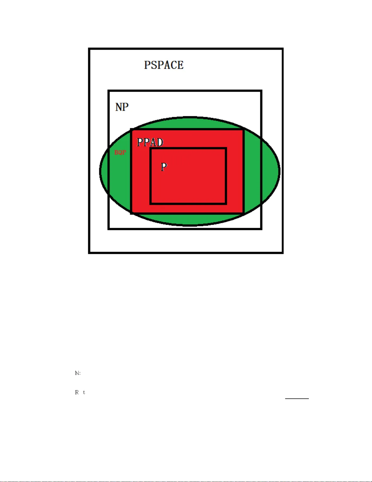
BQP and PP AD Y ang Daniel Li Octob er 22, 2018 Abstract W e initiate t he study of the relationship b et w een tw o co mplexit y class es, BQP ( B o unded- Erro r Q uan tum P olynomial-Time) and PP AD ( P olynomial P arity A rgument, D irected). W e first give a conjecture that PP AD is co n tained in BQP , and show a necessary and sufficien t condition for the conjecture to hold. Then we pro ve that the conjecture is not true under the oracle mo del. In the e nd, we raise some in ter e sting op en problems / future directions. 1 In tro d uction Quantum computing and alg orithmic game theory ar e t w o exciting and active areas in the last t wo decades. Quan tum co mputing lies in the intersection of computer science and quan tum ph ysics, and studies the p ow e r and limitation of a quantum computer. Algor ithmic game theory touches upon the foundations of both computer science and economics, and aims to desig n efficient alg orithms in strategic circumstances. If we want to come up with some examples that are able to demons trate the in terac tion b et ween computer science and other disciplines, then quantum computing and algor ithmic game theory a re t w o p erfect ca ndidates. Quantum mechanics may provide additio na l computationa l p o wer, and quantum computers can test the foundations of quantum mec hanics. Eco no mics lends so me strategic views , and computer science rewards with computational p oin ts of view. W e refer readers to [NC00] and [NR TV07] for more information. The cen tr al topics of quantum computing and alg orithmic game theory ar e the hardness of tw o complexity class es, BQP ( B ounded-Er ror Q uan tum P olynomial-Time) a nd PP AD ( P olynomial P arity A r g umen t, D irected). BQP , as in troduced by B e rnstein and V azarani [BV97], characterizes efficient computation of a q ua n tum computer and is the qua ntum a nalog of BPP . V er y little is known a bout BQP , and a wide b elief is that BQP a nd NP a re incomparable complexity clas ses [BBBV9 7, B V97, Aar10]. Papadimitriou intro duced the co mplexit y class PP AD [Pap94], which is a sp ecial c lass b etw een P and NP . Since then, the ha rdness of PP AD has a lso beco me a lo ngstanding op en pro blem. Although lots of important problems, say the problem of co mputing a Nas h equilibr ium ( NASH for s hort) [D GP09, CDT09], were s ho wn to be PP AD -complete, ther e ha v e b een very few relations from PP AD to other complexity classes. In this pap er, we initiate the study of the relations hip betw een BQP a nd PP AD . The representative pro blem o f PP AD is NA SH [Pap94], and the most well-kno wn pro blem in BQP is fac to ring [Sho97]. Both NASH and fac toring are in the complexit y clas s TFNP ( the set of total search problems, see [MP91]) in the sense that ev ery instance o f NASH and factoring alwa ys has a solution. Ther efore, it seems that there may b e some rela tionship betw een PP AD and BQP . In fa c t, this p ossible rela tion was (implicitly) men tioned in a talk given b y Papadimitriou ten years ago [Pap01]. Papadimitrious said tha t “together with factoring, the complexity of finding a Na s h equilibrium is in m y opinion the most imp ortant co ncrete open question on the bo undary of P to day”. In other words, Papadimitriou asked: do there ex ist (classically and deterministically) efficien t algorithms f or factoring and NASH ? As it hav e been shown tha t there exist e fficien t quant um alg orithms for factoring [Sho9 7], it is natural for us to ask: do there exist efficie nt quan tum a lgorithms for NASH ? Mor e gener ally , is PP AD co n tained in BQP ? Our co njecture is that PP AD is contained in BQP . F ormally , Conjecture 1 PP AD ⊆ BQP . The conceived relatio nship can b e illustrated by Figure 1, wher e the gr e en+r e d is BQP and the r e d denotes PP AD . W e will formally define quantum Na sh equilibrium, the quan tum analog of Nash equilibrium, and prov e the fact that PP AD is co n tained in BQP if and only if there exis ts a p olynomial- time quantum alg orithm for computing a quantu m Nash equilibrium. Therefore, to prov e the conjecture, w e need to find an efficien t (p olynomial-time) quant um alg orithm, and to disprov e the conjectur e , we have to sho w a super-p olynomial lower bound for the time complexity of computing a quan tum Nash equilibr ium. Another wa y to express the conjecture is that quantum computers can compute a Na sh equilibrium in p olynomial time, or that quantum co mputers can exponentially speed-up the computation of a Nash equilibrium. And we will r ule out this p ossibility under the o racle mo del. 1 Figure 1: Th e conceiv ed p icture The orga niz a tion of this pa per is as follows. Section 2 presents the definition of BQP and PP AD , and in Section 3, we in tro duce the no tion of quan tum Nash eq uilibrium and analyze it. Section 4 provides the nec e ssary and sufficien t condition for o ur c o njecture to hold. Section 5 pro v es a low er b ound of c omputing a Nash equilibrium using quan tum co mputers under the oracle model. And we co ncludes the pap er with some op en pr oblems/future dir ections in Section 6. 2 Preliminaries 2.1 Notation Some notations used throughout the pap e r are listed here. • N : the set o f natural num b ers, { 1 , 2 , 3 , . . . } . • [ n ]: the integer set { 1 , 2 , . . . , n } . • R : the set o f real num b ers. • || φ || : the 2- norm of a vector φ . If φ is a qua n tum state P x α x | x i , then || φ || = p P x | α x | 2 . 2.2 BQP [BV97] introduced the notion o f BQP , and a simplified v ersion is as follo ws. 2 Definition 1 A language L is in BQP if and only if ther e ex ists a p olynomia l-time un iform family of quantum cir cuits { Q n : n ∈ N } , such that • F or al l n ∈ N , Q n takes n qubits as input and outputs 1 bi t. • F or al l x in L , P r ( Q | x | ( x ) = 1) ≥ 2 / 3 . • F or al l x not in L , P r ( Q | x | ( x ) = 0) ≥ 2 / 3 . 2.3 PP AD and PP AD-completeness T otal search problems are pr oblems for which solutions are guar an teed to exist, and the challenge is to find a sp ecific so lution. In [Pap94], Papadimitriou defined the following total sear c h problem. Definition 2 (END-O F-THE-LINE) L et S (standing for S u c c essor) and P (standing for P r e de c essor) b e t wo p olynomial size cir cuits that given input strings { 0 , 1 } n output s t rings { 0 , 1 } n . We fur- ther r e quir e that P (0 n ) = 0 n 6 = S (0 n ) . The aim is to find an input x such that P ( S ( x )) 6 = x or S ( P ( x )) 6 = x 6 = 0 . A more intuitiv e descr iption of END-OF-THE- LINE is as follows. G is a (p ossibly e x ponentially large) dire c ted graph with no isolated v ertices, and with every vertex having at most one predecessor and one successor . G is sp ecified by giv ing a p olynomial-time computable function f ( v ) (p olynomial in the size of v ) that returns the predecessor and successo r (if they exist) of the vertex v . Given a vertex s in G with no predecessor , find a vertex t 6 = s with no predeces sor or no successor. (The input to the problem is the source vertex s and the function f ( v )). In other words, we want a n y source or sink of the directed gra ph other than s . PP AD was defined based on this problem. Definition 3 ( PP AD ) The c omplexity class PP AD c ontains al l total se ar ch pr oblems r e- ducible to END-OF-THE-LINE in p olynomial time. PP AD -co mpleteness was also defined. Definition 4 ( PP AD -c ompleteness) A pr oblem is c al le d PP AD -c omplete if it is in PP AD and al l pr oblems in PP AD c an re duc e to it in p olynomia l t ime. 3 Quan tum Nash Equilibrium 3.1 Classical Equilibria First, we review classical Nash equilibria and co rrelated e q uilibria, all of which ca n b e fo und in [NR TV07]. In a clas sical game there ar e n play er s, labele d { 1 , 2 , . . . , n } . Each pla y er i has a set S i of strategies. W e us e s = ( s 1 , . . . , s n ) to denote the vector of stra tegies se lected b y the play ers a nd S = × i S i to denote the set of all po ssible join t strategies. Each player i has a utilit y function u i : S → R , giving the pay off or utilit y u i ( s ) to player i on the joint strategy s . There is a solution concept called Nash equilibrium, in which the equilibrium strategies a re known by all play er s, and no play er can gain more by unilater ally mo difying his or her choice. F ormally , Definition 5 A mixed Nash equilibrium is a pr ob ability ve ctor p = p 1 × . . . × p n for some pr ob ability distribut ions p i ’s over S i ’s satisfying that X s − i p − i ( s − i ) u i ( s i , s − i ) ≥ X s − i p − i ( s − i ) u i ( s ′ i , s − i ) , ∀ i ∈ [ n ] , ∀ s ′ i ∈ S i , ∀ s i ∈ S i s.t. p i ( s i ) > 0 , where s − i is the s trategies c hosen by pla y ers but play e r i , a nd p − i denotes the probability distribution ov er s − i . Informally sp eaking, for a mixed Na s h equilibrium, the exp ected pay o ff ov e r pr o babilit y distribution o f s − i is maximize d, i.e. E s − i [ u i ( s i , s − i )] ≥ E s − i [ u i ( s ′ i , s − i )]. 3 W e can further relax the Nash condition and define an ǫ -approximate Na s h equilibr ium to b e a profile of mixed strateg ies such that no player c an g ain more than ǫ amo unt by changing his / her own s trategy unilaterally . F or mally , Definition 6 An ǫ -a pproximate Nash equilibrium is a pr ob ability ve ctor p = p 1 × . . . × p n for some pr ob ability distributions p i ’s over S i ’s satisfying that X s − i p − i ( s − i ) u i ( s i , s − i ) ≥ X s − i p − i ( s − i ) u i ( s ′ i , s − i ) − ǫ , ∀ i ∈ [ n ] , ∀ s ′ i ∈ S i , ∀ s i ∈ S i s.t. p i ( s i ) > 0 , where ǫ > 0. In addition, the probability distribution of eac h player may not be indep enden t, but cor related, forming the notion of correlated equilibria. Definition 7 A corr elated eq uilibrium is a pr ob ability distribution p over S satisfying that X s − i p ( s i , s − i ) u i ( s i , s − i ) ≥ X s − i p ( s i , s − i ) u i ( s ′ i , s − i ) , ∀ i ∈ [ n ] , ∀ s i , s ′ i ∈ S i . Notice that a correlated equilibrium p is a Nash equilibr ium if and only if p is a pr oduct distribution. 3.2 Quan tum Equilibria This pa rt gener a lizes classical eq uilibria to quan tum equilibria, where players are allow ed to use “ quan tum” strategie s . T o be more precise, each pla yer i now has a Hilb e r t space H i = span { s i : s i ∈ S i } , and the joint stra tegy can be an y quantum s ta te ρ in H = ⊗ i H i . The pay o ff/utilit y for pla y er i on joint strategy ρ is µ i ( ρ ) = E [ u i ( s ( ρ ))] = P s h s | ρ | s i u i ( s ), where s ( ρ ) is the outco me pure strategy when ρ is measured according to the c o mputational bas is { s : s ∈ S } . Note that what each play er i can do is to apply an a dmissible super -op e r ator Φ i on her own space H i . W e s ometimes write Φ i for Φ i ⊗ I − i . W e use C P T P ( X ) to denote the set of all admissible (completely p ositive and trace preserving) sup er-op erators on a space X . The notions of quan tum Nash equilibr ia and quantum corr elated equilibria ar e defined as follows. Definition 8 A quant um Nash equilibrium is a quantum st r ate gy ρ = ρ 1 ⊗ . . . ⊗ ρ n for ρ i ’s in H i ’s satisfying X s h s | ρ | s i u i ( s ) ≥ X s h s | Φ i ( ρ ) | s i u i ( s ) , ∀ i ∈ [ n ] , ∀ Φ i ∈ C P T P ( H i ) Definition 9 A quantum correla ted equilibrium is a quantum str ate gy ρ in H satisfying X s h s | ρ | s i u i ( s ) ≥ X s h s | Φ i ( ρ ) | s i u i ( s ) , ∀ i ∈ [ n ] , ∀ Φ i ∈ C P T P ( H i ) 3.3 Relations b et w een Classical and Quan tum Equilibria This section studies the relation b et w een classical and quantum equilibr ia. A quan tum mixed state ρ naturally induces a classical distribution p ov er S defined by p ( s ) = ρ ss (1) While taking diagonal entries seems to b e the most natural mapping from q ua n tum states to classical distributions , there a re more optio ns for the mapping in other direction. Giv en a classical distributio n p ov er S , w e can co nsider 1. ρ ( p ) = P s p ( s ) | s ih s | , 2. | ψ ( p ) i = P s p p ( s ) | s i , or 3. an y densit y matrix ρ with p ( s ) = ρ ss satisfied. 4 W e w ant to study whether equilibr ia in o ne world, clas sical or q uan tum, implies equilibria in the other w orld. The following theorem says that qua n tum alwa ys implies classical. Theorem 3. 1 If ρ is a quantum c orr elate d e quilibrium, then p define d by p ( s ) = ρ ss is a classic al c orr elate d e quilibrium. In p articular, if ρ is a quantum Nash e quilibrium, then p is a classic al Nash e quilibrium. Pro of : See the app endix. The implication from classical to quantum is muc h more complicated. The following theorem says tha t the first mapping alwa ys giv es a qua n tum equilibrium. That is, the utility of i cannot be increas e d for a classical equilibrium even when play er i is allow ed to hav e quantum o pera tions. Theorem 3. 2 If p is a classic al c orr elate d e qu ilibri um, then ρ = Σ s ∈ S | s ih s | is a quantu m c orr elate d e quilibrium. In p articular, if p is a classic al Nash e quilibrium, then ρ as define d is a quantum Nash e quilibrium. Pro of : See the app endix. F ollowing this result, we a re a ble to g iv e a n affirmativ e answ er to a n imp ortant pr oblem, whether quantum Nash eq uilibria alwa ys exist. Corollary 3. 3 F or al l standar d game G with fin ite numb er of play ers and str ate gies, quantum Nash e quilibria always exist. Pro of : See the app endix. The second wa y of inducing a qua n tum state is in teresting: It pr e s erves (unco r related) Nash equilibria, but does not prese r v e cor related Nash e q uilibria in gener al. Theorem 3. 4 Ther e exists a classic al c orr elate d e quilibrium p with | ψ i = P s p p ( s ) | s i not b eing a quant um c orr elate d e quilibrium. However, if p is a classic al N ash e qu ilibrium, then | ψ i = P s p p ( s ) | s i is a quantum Nash e quilibrium. Pro of : See the app endix. Finally , for the third mapping, i.e. a g eneral ρ with p ( s ) = ρ ss satisfied, the eq uilibr ium prop erty can be heavily destroyed, even if p is unco rrelated. (A ctually , we will show suc h counterexamples even for t w o-play er symmetric games.) Theorem 3. 5 Ther e exist ρ and p satisfying that p ( s ) = ρ ss , p is a classic al Nash e quilibrium, but ρ is not even a qu ant um cor related e quilibrium. Pro of : See the app endix. Despite of t he ab ov e fact, one should not think that the la rge range of the third t ype of mappings always enables s ome mapping to destroy the equilibria. Theorem 3. 6 Ther e exist classic al c orr elate d e quilibria p , such that al l quantu m s t ates ρ with ρ ss = p ( s ) ar e quantum c orr elate d e quilibria. Pro of : See the app endix. 4 A Necessary and Sufficien t Condition In this section, we prov e the following theorem. Theorem 4. 1 PP AD ⊆ BQP if and only if ther e exists a p olynomial-time quantum algorithm for finding a quantum Nash e quilibrium. Pro of : If PP AD ⊆ BQP , then for a ga me G , there exis ts a po lynomial-time quantum algorithm for finding a Nash equilibrium p , since finding a Nash equilibrium is a PP AD -co mplete pro blem. As s ho wn in the pr oo f of Co rollary 3.3, we can alwa ys conv e r t p to a quan tum equilibr ium ρ 5 in p olynomial time. Hence, there exists a p olynomial- time quantum algorithm for finding a quantum Nash equilibrium. Next we will pr o ve the in verse direction for the statement. W e define a new problem as follo ws. Definition 10 SAMPLE-NASH is a se ar ch pr oblem t hat, on input a game G , outputs a pur e str ate gy s s ample d fr om a fixe d Nash e qu ilibri um p of the game G . Suppo se that we a re given a ga me G and we find a quantum Nas h eq uilibr ium ρ in p olynomial- time using the q ua n tum alg orithm. Here w e as sume that the induced cla ssical proba bilit y distribution induced from ρ is p , defined b y p ( s ) = ρ ss . By measuring ρ according to the com- putational bas is { s : s ∈ S } , w e can obtain a pure strategy s , whic h is sampled accor ding to p . According to Theorem 3.1, p is a classical Nash equilibrium, and therefore s is a n output fo r SAMPLE-NASH . So w e are able to obtain the output for SAMPLE-NASH in p olynomia l time. Now we hav e a p olynomial-time quantum algorithm for SAMPLE-NASH . W e ha v e the fo llo wing result, which is to be prov ed la ter . Lemma 4. 2 A PP AD -c omplete pr oblem c an b e r e duc e d to SAMPLE-NASH in r andomize d p olynomial time. Therefore, we have a polyno mial-time quan tum algorithm fo r a PP AD - complete problem, implying PP AD ⊆ BQP . 4.1 Pro of of Lemma 4.2 T o pro ve Lemma 4.2, w e use the following r esult. Lemma 4. 3 [CDT09] F or any c onstant c > 0 , the pr oblem of c omputing a 1 /m c -appr oximate Nash e quilibrium of a p ositively normalize d 1 m × m bima trix game is PP AD -c omplete. W e just need to re duce the problem in Lemma 4.3, to SAMPLE-NASH in randomized po lynomial time. F or a n instance o f the problem in Lemma 4.3, namely a p ositively normalized m × m bimatrix game G , we use G as the input for S AMPLE-NASH . W e assume tha t w e ha v e an algorithm A for SAMPLE-NASH , and we w ant to use A to construct a n algor ithm fo r the problem in Lemma 4.3 in r andomized p olynomial time. Suppos e the output of A is sampled from a Nash equilibrium p = p 1 × p 2 . Lemma 4. 4 Supp ose that p = p 1 × p 2 is a Nash e quilibrium of a p ositively normalize d m × m bimatrix game G , and t hat the output of A, an algorithm for SAMPLE-NASH , is sample d fr om p . F or any ǫ = O (1 /m c ) , with high pr ob ability, we wil l get a pr ob ability distribution q = q 1 × q 2 with || q 1 − p 1 || 1 ≤ ǫ and || q 2 − p 2 || 1 ≤ ǫ , after running A fo r O ( m 2 ǫ − 2 ) times. Lemma 4. 5 Supp ose that p = p 1 × p 2 is a Nash e quilibrium of a p ositively normalize d m × m bimatrix game G . Any pr ob ability distribution q = q 1 × q 2 with || q 1 − p 1 || 1 ≤ ǫ and || q 2 − p 2 || 1 ≤ ǫ , is a 2 ǫ -appr oximate Nash e quilibrium of game G . By Lemma 4.4, we can run a lgorithm A for O ( m 2 ǫ − 2 ) times to construct a desired probability distribution q with hig h pr o babilit y . By Lemma 4 .5, q is an 2 ǫ -approximate Nash eq uilibrium. T o find an 1 /m c -approximate Nash equilibrium, w e need to use A for O ( m 2 c +2 ) times, whic h is p olynomial in input size 2 m 2 . 1 In [CDT09], the game matrices are normalized in t he sense that all the entries are b etw een 0 and 1 (positively normalized), or b etw een − 1 and 1. 6 4.1.1 Pro of of Lemma 4.4 W e as sume that player 1’s m stra teg ies are s 1 , s 2 , . . . , s m . Define k = ⌈ 4000 m 2 /ǫ 2 ⌉ = O ( m 2 ǫ − 2 ). F or each i ∈ [ k ], j ∈ [ m ], define random v ariable X ij taking v alues in { 0 , 1 } , where X ij = 1 with pro babilit y p 1 ( s j ). Suppo se that ǫ j = ǫ 2 m for each j ∈ [ m ]. Define rando m v aria bles X j to be X j = P i ∈ [ k ] X ij k for each j ∈ [ m ]. By Cher noff bo und, P r ( X j ≥ p 1 ( s j ) + ǫ j ) ≤ e − 2 ǫ 2 j k (2) and P r ( X j ≤ p 1 ( s j ) − ǫ j ) ≤ e − 2 ǫ 2 j k . (3) Define a pr obability vector q 1 to b e ( X 1 , . . . , X m ), whic h is a distribution o v er strategies ( s 1 , s 2 , . . . , s m ). It is ea s ily chec k a ble that P j X j = 1 and that P r ( || q 1 − p 1 || 1 ≤ X j ∈ [ m ] | X j − p 1 ( s j ) | ≤ X j ∈ [ m ] ǫ j ≤ ǫ ) ≥ 1 − X j ∈ [ m ] 2 e − 2 ǫ 2 j k (4) ≥ 0 . 9 95 . (5) Similarly , we can g et q 2 satisfying || q 2 − p 2 || 1 ≤ ǫ with probability at lea s t 0 . 995 . By union bo und, we can get the desired q with probability at least 0 . 99. 4.1.2 Pro of of Lemma 4.5 F or all i in { 1 , 2 } , for all s ′ i in the set of stra tegies of pla y er i , and for all s i in the supp ort of the set of strategie s o f pla yer i , w e hav e the following: X s − i q − i ( s − i ) u ( s ′ i s − i ) − X s − i q − i ( s − i ) u ( s i s − i ) = X s − i p − i ( s − i ) u ( s ′ i s − i ) + X s − i ( q − i ( s − i ) − p − i ( s − i )) u ( s ′ i s − i ) − X s − i q − i ( s − i ) u ( s i s − i ) ≤ X s − i p − i ( s − i ) u ( s i s − i ) + || q − i − p − i || 1 max s u ( s ) − X s − i q − i ( s − i ) u ( s i s − i ) ≤ X s − i p − i ( s − i ) u ( s i s − i ) + ǫ × 1 − X s − i q − i ( s − i ) u ( s i s − i ) ≤ X s − i ( p − i ( s − i ) − q − i ( s − i )) u ( s i s − i ) + ǫ ≤|| q − i − p − i || 1 max s u ( s ) + ǫ ≤ ǫ × 1 + ǫ ≤ 2 ǫ F ollowing the definition of a pproximate Nash equilibrium, q is a 2 ǫ -approximate Nas h equi- librium of G . 5 A Lo w er Bound un der the Oracle M o del 5.1 The Oracle Model The oracle model is also called black-box mo del, or relativiz ed mo del, a nd is one of simplest mo dels in c o mputer science. Suppos e that there is a bo olean function f : [ N ] → { 0 , 1 } , and 7 that f can b e computed in p olynomial time. W e w an t to find an x ∈ [ N ], suc h that f ( x ) = 1. In the context of PP AD -complete problems, N , which could b e exp o nen tial in the size of the input, is the num b er o f points in the search space, and f ( x ) = 1 for x ∈ [ N ] means that x is the answer w e desire. F or a PP AD -complete problem, ther e always exis ts an x ∈ [ N ], suc h that f ( x ) = 1, and the que s tion is that we do not know wher e it is. Suc h an f is ca lle d a n oracle, and we w ant to compute an x ∈ [ N ], such that f ( x ) = 1. In an or acle mo del, alg orithms are allow ed to mak e q ue r ies to the oracle but ar e pr ohibited to take adv antage of what underlie s the ora cle. Since w e use q ua n tum algorithms here, w e can also ma k e use of quantum s uperp osition. F or instance, for a quantum state P x α x | x i , we fir st add some ancilla qubits, obtaining P x α x | x i| 0 i , and then mak e a single query to the oracle, getting P x α x | x i| f ( x ) i . In summary , in the oracle mo del, the function f can b e seen as the input, and we need to design a quantum algorithm to find a so lution x ∈ [ N ] with f ( x ) = 1, which is guaranteed to exist. The time co mplexit y is what we care a nd is defined to the num b er of queries made to the oracle. 5.2 The Lo wer Bound W e use a hybrid argument of [BBBV97, V az04] to show a r e sult when there is only one x ∈ [ N ] such that f ( x ) = 1, na mely for the problems with a single so lution. Hybrid a rgument is from a classic paper b y Y ao [Y a o82], and later has numerous applications in cryptography and complexity theory [BM84, GL89, HILL99, INW94, Nis91, Nis92, NW94]. Th us, our pro of is not new, and existing techniques are eno ugh to prov e the result. This is pa r tly due to the fact that the or acle model is very w ell-studied. Theorem 5. 1 Under the or acle mo del, to solve a PP AD -c omplete pr oblem with a single solu- tion, any quantum algorithm has t o make at le ast Ω( √ N ) queries to the or acle. Pro of : Suppo se A is a n (arbitrary) algo rithm under the oracle mo del, and it makes k queries to the input o racle. If k = Ω( N ), then everything is done and w e need to do no thing. So a rea sonable assumption is that k = o ( N ). W e define an a uxiliary or acle function h : [ N ] → { 0 , 1 } w ith h ( y ) = 0 for all y ∈ [ N ]. Such an oracle cannot characterize an y PP AD -c o mplete problem, as ther e are alw ays so lutions for PP AD -co mplete problems while here h means no solution at all. So we use h just purely for analysis. Run A on h a nd w e call such a run A h . Le t P y : y ∈ [ N ] α y ,t | y i be the query at time t ∈ [ k ], and let the query magnitude of y to b e P t ∈ [ k ] | α y ,t | 2 . It is not hard to see that the expected query magnitude o ver all possible y is E y ( P t | α y ,t | 2 ) = k / N . W e ha v e the following claim. Claim 1 Ther e exist z 1 , z 2 ∈ [ N ] with z 1 6 = z 2 , such that P t | α z 1 ,t | 2 ≤ ( k + 1) / N and P t | α z 2 ,t | 2 ≤ ( k + 1) / N . By Cauch y-Sch wartz inequality , we kno w tha t P t | α z 1 ,t | ≤ ( k + 1) / √ N a nd that P t | α z 2 ,t | ≤ ( k + 1) / √ N . Let φ h,t , t ∈ [ k ] be the states of A h after the t -th step. W e define tw o or acles g 1 : [ N ] → { 0 , 1 } and g 2 : [ N ] → { 0 , 1 } : • g 1 ( z 1 ) = 1 and for all y 6 = z 1 , g 1 ( y ) = 0; • g 2 ( z 2 ) = 1 and for all y 6 = z 2 , g 2 ( y ) = 0. g 1 and g 2 are the le gal inputs of A and corresp ond to PP AD -complete pro ble ms . Now run the algorithm A on g 1 (the run is denoted as A g 1 ) and supp ose the final state of A g 1 is φ g 1 ,k . By hybrid a rgument, we hav e the following claim. Claim 2 [V az04] φ h,k − φ g 1 ,k = P k t =1 E t , wher e || E t || ≤ √ 2 | α z 1 ,t | . 8 Along with the triangle inequalit y , we hav e || φ h,k − φ g 1 ,k || ≤ X t || E t || ≤ √ 2 X t | α z 1 ,t | ≤ ( k + 1) p 2 / N . (6) Similarly , if we run the a lgorithm A o n g 2 (the r un is denoted as A g 2 ) and the final state of A g 2 is φ g 2 ,k , then a hybrid argument and the tria ngle inequality could show that || φ h,k − φ g 2 ,k || ≤ ( k + 1) p 2 / N . (7) If we apply the triangle inequality for a nother time, we get || φ g 1 ,k − φ g 2 ,k || ≤ 2( k + 1) p 2 / N , (8) implying that φ g 1 ,k and φ g 2 ,k can b e distinguished w ith probability at most O ( k / √ N ). Since z 1 6 = z 2 , if A can solve problems cor resp onding to g 1 and g 2 , namely if A can find z 1 and z 2 , it should at leas t distinguis h g 1 and g 2 , and a lso φ g 1 ,k and φ g 2 ,k with some constan t proba bilit y . As a r esult, A should at lea st make Ω( √ N ) queries. When there are multiple solutions, say p solutions, then k = Ω( p N /p ), whic h is a s tr aight - forward gener alization from the theorem ab ov e. More fo rmally , Corollary 5. 2 Under the or acle mo del, to solve a PP AD -c omplete pr oblem with p solut ions, any quantum algo rithm has to make at le ast Ω( p N /p ) queries t o the or acle. 5.2.1 Pro of of Claim 1 Let us suppose that ther e do es n ot ex ist z 1 , z 2 ∈ [ N ] with z 1 6 = z 2 , such that P t | α z 1 ,t | 2 ≤ ( k + 1) / N and P t | α z 2 ,t | 2 ≤ ( k + 1) / N . This means there is a t mo st one z ∈ [ N ] such that P t | α z ,t | 2 ≤ ( k + 1) / N , and for all y 6 = z , y ∈ [ N ], P t | α y ,t | 2 > ( k + 1) / N . Th us, X y : y ∈ [ N ] X t | α y ,t | 2 = X y : y 6 = z X t | α y ,t | 2 + X t | α z ,t | 2 ≥ X y : y 6 = z X t | α y ,t | 2 > ( N − 1 ) × ( k + 1) / N = k + 1 − ( k + 1) / N > k . (9) But we hav e already known that E y : y ∈ [ N ] ( X t | α y ,t | 2 ) = k/ N , (10) and that X y : y ∈ [ N ] ( X t | α y ,t | 2 ) = k. (11) The inequa lit y (9) and the eq ua tion (11) exhibit clear cont radiction. Consequently , our a ssump- tion that there do es not exist z 1 , z 2 ∈ [ N ] with z 1 6 = z 2 , such that P t | α z 1 ,t | 2 ≤ ( k + 1 ) / N and P t | α z 2 ,t | 2 ≤ ( k + 1) / N is incorrect. This completes the proo f of Claim 1. 9 6 Concluding Rema rks On the one ha nd, it seems that the w ell-studied oracle model pres en ts us an insurmountable obstacle tow a rds an ex ponentially sp eed-up using quantum computers for computing PP AD - complete problems. If we wan t to make a step c lo ser to prove our conjectur e that PP AD is contained in BQP , w e have to get rid of ora cles and design new structures tha t ca n provide more information. W e b elieve that this ma y need fundamen ta l re v olution in the field o f quantum computing. T he theory comm unit y has spent lots o f effort in designing qua n tum algorithms for factoring as well as graph isomor phis m, t w o sp ecial problems b etw een P and NP . And now it is the time that we turn our atten tion to the third sp ecial problem, NA SH , or more generally PP AD -co mplete problems. On the o ther hand, it seems that purely exploiting the potential of qua ntum sup erp osition is not enough, and quantum e ntanglement may play a more impor tan t role as a re source for quantum computation. It is w ell-known that quantum information theory relies on entangle- men t in tw o quite differen t contexts: as a r esource for qua n tum computation and as a so urce for nonloca l correlations amo ng different parties. It is s tr ange and not under stoo d that entan- glement is cr ucially linked with nonlo cality but not with computation. Quantum computation and nonlo c alit y are t w o faces of en tanglement , and more connections sho uld be established in the future. 7 Ac kn o wledgmen ts Thanks to Shengyu Zhang for discussions at the early stage of this w ork. 10 References [Aar10] Scott Aar onson. BQ P and the po ly nomial hierarch y . Pr o c e e dings of t he 42nd Annual ACM symp osium on The ory of Computing , 201 0. [BBBV97] Charles Be nnett, Ethan Bernstein, Gilles Br a ssard, and Umesh V azirani. Str e ngths and weaknesses of qua n tum computing. SIAM Journal on Computing , 26(5):151 0– 1523, 19 97. [BM84] Manuel Blum and Silvio Micali. How to genera te cry ptographically stro ng sequences of pseudo-r andom bits. SIAM J. Comput. , 13(4):85 0–864, 1 984. [BV97] Ethan Ber nstein and Umesh V azirani. Quantum complexity theory . SIAM Journal on Computing , 26 (5 ):1411–14 73, 1997. [CDT09] Xi Chen, Xiaotie Deng, and Shang-Hua T eng. Se ttling the co mplexit y of computing t wo-pla y er Nas h equilibria. Journal of A CM , 56, 20 09. [DGP09] Constan tinos Dask alakis, Paul Goldb erg, and Christos Papadimitriou. The complex- it y of computing a Nash equilibrium. SIAM Journal on Computing , 39(1):195– 259, 2009. [GL89] Oded Goldr eic h and Leonid A. Levin. A hard-core predicate for all one-way func- tions. In STOC , pa ges 25– 32, 19 89. [HILL99] Johan H ˚ astad, Russe ll Impag liazzo, Le onid A. Levin, and Mic hael Lub y . A pse udo - random g enerator from a n y one-wa y function. SIAM J. Comput. , 28(4):1364–1 396, 1999. [INW94] Russell Impagliazzo, Noam Nisan, and Avi Wigderson. P seudorandomness for net- work a lgorithms. In STOC , pag es 356– 364, 199 4. [MP91] Nimro d Megiddo and Christos Papadimitriou. On total functions, e x istence theo- rems, and computationa l complexity . The or etic al Computer Scienc e , 81 (2):317 –324 , 1991. [NC00] Mic hael Nielsen and Is aac Ch uang. Quantum Computation and Quantu m Informa- tion . Cam bridge Universit y Press, 20 00. [Nis91] Noam Nisan. Pseudora ndom bits for cons ta n t depth circuits. Combinatoric a , 11(1):63– 70, 199 1. [Nis92] Noam Nisa n. Pseudora ndo m genera tors for space- bounded computation. C ombina- toric a , 1 2(4):449–4 6 1, 1992 . [NR TV07] Noam Nisan, Tim Roug hgarden, Ev a T ar dos, and Vijay V a zirani. Alg orithmic Game The ory . Cambridge Univ ersity Pr ess, 2007. [NW94] Noam Nisan and Avi Wigderson. Hardness vs randomnes s . J. Comput. Syst. Sci. , 49(2):149 –167, 199 4. [Pap94] Christos Papadimitriou. On the co mplexit y of the parity ar gumen t and other ineffi- cient pro ofs of existence. Journal of Computer and Syst em Scienc es , 48(3):49 8–532, 1994. [Pap01] Christos H. Papadimitriou. Alg o rithms, games, and the in ternet. In S TOC , pages 749–7 53, 200 1 . [Sho97] P eter Shor . P olynomial-time algorithms for prime factorization a nd discr ete lo g- arithms on a qua n tum computer. SIAM Journ al on Computing , 2 6(5):1484–1 509, 1997. [V az04 ] Umesh V azirani, 2004. Lecture Notes of Quan tum Computing. [Y ao8 2] Andrew Chi- Chih Y ao . Theory and applications of trap do or functions (extended abstract). In FOCS , pages 8 0–91, 1982. A Pro of of T h eorem 3.1 Recall tha t we are given that µ i ( ρ ) ≥ µ i (Φ i ( ρ )) for all play er s i and all admissible supe r- op erators Φ i on H i , a nd w e wan t to prov e that for all play er s i and all strategies s i , s ′ i ∈ S i , X s − i p ( s i , s − i ) u i ( s i , s − i ) ≥ X s − i p ( s i , s − i ) u i ( s ′ i , s − i ) (12) for p ( s ) = ρ ss . Fix i and s i , s ′ i . Consider the a dmissible sup er-op erator Φ i defined by Φ i = X t i 6 = s i P t i ρP t i + ( s i ↔ s ′ i ) P s i ρP s i ( s i ↔ s ′ i ) (13) where P t i is the pro jection onto the subspace span ( t i ) ⊗ H − i , and ( s i ↔ s ′ i ) is the operato r swapping s i and s ′ i . It is not hard to verify that Φ i is an admissible sup er-op erato r. Next w e will show tha t the difference of µ i ( ρ ) and µ i (Φ i ( ρ )) is the same as that of the t w o s ides of Eq. (12). µ i ( ρ ) = E [ u i ( s ( ρ ))] = X ¯ s ∈ S h ¯ s | ρ | ¯ s i u i ( ¯ s ) = X ¯ s ∈ S p ( ¯ s ) u i ( ¯ s ) = X ¯ s i 6 = s i X ¯ s − i p ( ¯ s ) u i ( ¯ s ) + X ¯ s − i p ( s i ¯ s − i ) u i ( s i ¯ s − i ) (14) µ i (Φ i ( ρ )) = X ¯ s ∈ S h ¯ s | Φ i ( ρ ) | ¯ s i u i ( ¯ s ) = X ¯ s ∈ S h ¯ s | X t i 6 = s i P t i ρP t i + ( s i ↔ s ′ i ) P s i ρP s i ( s i ↔ s ′ i ) | ¯ s i u i ( ¯ s ) = X ¯ s ∈ S h ¯ s | X t i 6 = s i P t i ρP t i | ¯ s i u i ( ¯ s ) + X ¯ s ∈ S h ¯ s | ( s i ↔ s ′ i ) P s i ρP s i ( s i ↔ s ′ i ) | ¯ s i u i ( ¯ s ) = X t i 6 = s i X ¯ s − i p ( t i ¯ s − i ) u i ( t i ¯ s − i ) + X ¯ s − i p ( s i ¯ s − i ) u i ( s ′ i ¯ s − i ) (15) Since ρ is a quantum corr elated equilibrium, w e have µ i ( ρ ) ≥ µ i (Φ i ( ρ )). Comparing t he ab o ve tw o expressions for µ i ( ρ ) and µ i (Φ i ( ρ )) g iv es Eq. (12) as desired. B Pro of of T h eorem 3.2 Let α ( s i ) = P s − i p ( s i , s − i ) u i ( s i , s − i ) and β ( s i , s ′ i ) = P s − i p ( s i , s − i ) u i ( s ′ i , s − i ). Now for any i , we have µ i ( ρ ) = X s h s | ρ | s i u i ( s ) = X s p ( s ) u i ( s ) = X s i X s − i p ( s i s − i ) u i ( s i s − i ) = X s i α ( s i ) (16) where the first t wo s teps are b y the definition of µ i and p . Now for an arbitr ary TPCP sup er- op erator Φ i , we use its Kraus repres en tation to obtain Φ i ( ρ ) = k X j =1 ( A ij ⊗ I − i ) ρ ( A ∗ ij ⊗ I − i ) (17) with constraint P k j =1 A ∗ ij A ij = I i , wher e I i is the identit y sup er-op erator from L ( H i ) to L ( H i ). Now we hav e µ i (Φ i ( ρ )) = X s ′ h s ′ | Φ i ( ρ ) | s ′ i u i ( s ′ ) // by the def of µ i = X s ′ h s ′ | k X j =1 ( A ij ⊗ I − i ) ρ ( A ∗ ij ⊗ I − i ) | s ′ i u i ( s ′ ) = X s ′ k X j =1 h s ′ | ( A ij ⊗ I − i )( X s p ( s ) | s ih s | )( A ∗ ij ⊗ I − i ) | s ′ i u i ( s ′ ) // by the def of ρ = X s ′ X s k X j =1 h s ′ | A ij ⊗ I − i | s ih s | A ∗ ij ⊗ I − i | s ′ i p ( s ) u i ( s ′ ) = X s ′ i X s k X j =1 h s ′ i | A ij | s i ih s i | A ∗ ij | s ′ i i p ( s i s − i ) u i ( s ′ i s − i ) = X s ′ i X s i k X j =1 h s ′ i | A ij | s i ih s i | A ∗ ij | s ′ i i β ( s i , s ′ i ) // by the def of β ( s i , s ′ i ) Note that h s ′ i | A ij | s i ih s i | A ∗ ij | s ′ i i = k h s ′ i | A ij | s i ik 2 ≥ 0, th us b y the assumption that β ( s i , s ′ i ) ≤ α ( s ′ i ) (i.e. p is a class ic al c o rrelated equilibrium), w e hav e µ i (Φ i ( ρ )) ≤ X s i k X j =1 X s ′ i h s ′ i | A ij | s i ih s i | A ∗ ij | s ′ i i α ( s i ) = X s i k X j =1 h s i | A ∗ ij ( X s ′ i | s ′ i ih s ′ i | ) A ij | s i i α ( s i ) = X s i h s i | k X j =1 A ∗ ij A ij | s i i α ( s ′ i ) = X s i h s i | s i i α ( s i ) = µ i ( ρ ) where the last equality is by Eq. (16). This completes the pro of of T he o rem 3.2. B.1 Pro of of Corollary 3.3 W e will reduce the e x istence of a quantum Nash equilibrium to the existence of a Nas h equilib- rium. F or a given game G with finite players and finite s trategies, there alw ays exists a Nash equi- librium, say p . W e transform p into a quan tum s tate ρ using the the mapping ρ = P s p ( s ) | s ih s | . By Theor em 3.2, ρ is guara nteed to be quantum Nash equilibrium of G . Thu s, q ua n tum Nash equilibria alw a ys exist. C Pro of of Theorem 3.4 C.1 Examples of the First Statemen t Define utility functions of Play er 1 and 2 to b e: A =  270 126 0 270  . Suppo se the initial state is | ψ i = p 1 / 3 | 00 i + p 1 / 6 | 01 i + p 1 / 6 | 10 i + p 1 / 3 | 11 i , whose co r resp onding densit y matrix is ρ =     1 / 3 p 1 / 18 p 1 / 18 1 / 3 p 1 / 18 1 / 6 1 / 6 p 1 / 18 p 1 / 18 1 / 6 1 / 6 p 1 / 18 1 / 3 p 1 / 18 p 1 / 18 1 / 3     , and who se corresp onding classica l co rrelated distribution is p =  1 / 3 1 / 6 1 / 6 1 / 3  , which is easily verified to b e a classical cor related equilibrium. How ever, ρ is not a q uan tum Nash eq uilibr ium. Define a unitary matrix G =  p 2 / 3 p 1 / 3 p 1 / 3 − p 2 / 3  . Consider ρ ′ = ( G ⊗ I ) ρ ( G ⊗ I ) =     1 / 2 √ 2 / 3 0 − 1 / 6 √ 2 / 3 4 / 9 0 − √ 2 / 9 0 0 0 0 − 1 / 6 − √ 2 / 9 0 1 / 18     . It is easily seen that ρ ′ has higher expected utilit y v a lue for play er 1, ac tua lly µ 1 ( ρ ′ ) = 206 , µ 1 ( ρ ) = 201 . C.2 Pro of of the Second Statemen t Let ρ = | ψ ih ψ | = P a,b p p ( a ) p ( b ) | a ih b | . Then µ i ( ρ ) = X s h s | ρ | s i u i ( s ) = X s h s | X a,b p p ( a ) p ( b ) | a ih b || s i u i ( s ) = X s p ( s ) u i ( s ) = X s i p i ( s i ) X s − i p − i ( s − i ) u i ( s i , s − i ) = X s i : p i ( s i ) > 0 p i ( s i ) X s − i p − i ( s − i ) u i ( s i , s − i ) Now a ssume that Player i applies an a dmissible sup er-op erator Φ i on ρ : Φ i ( ρ ) = k X j =1 ( A ij ⊗ I − i ) ρ ( A ∗ ij ⊗ I − i ) where P k j =1 A ∗ ij A ij = I i . Let ¯ s i be a stra tegy s.t. p i ( ¯ s i ) > 0. Then b y the definitio n of Nas h equilibrium, we hav e X s i p − i ( s − i ) u i ( s i s − i ) ≤ X s i p − i ( s − i ) u i ( ¯ s i s − i ) , (18) for any s i . µ i (Φ i ( ρ )) = X s h s | Φ i ( ρ ) | s i u i ( s ) = X s h s | k X j =1 ( A ij ⊗ I − i ) ρ ( A ∗ ij ⊗ I − i ) | s i u i ( s ) = X s h s | k X j =1 ( A ij ⊗ I − i ) X a,b p p ( a ) p ( b ) | a ih b | ( A ∗ ij ⊗ I − i ) | s i u i ( s ) = X s,a,b,j p p ( a ) p ( b ) h s | ( A ij ⊗ I − i ) | a ih b | ( A ∗ ij ⊗ I − i ) | s i u i ( s ) = X s,a,b,j p p i ( a i ) p i ( b i ) p p − i ( a − i ) p − i ( b − i ) h s i | A ij | a i ih s − i | a − i ih b i | A ∗ ij | s i ih b − i | s − i i u i ( s ) = X s i ,s − i ,a i ,b i ,j p p i ( a i ) p i ( b i ) h s i | A ij | a i ih b i | A ∗ ij | s i i p − i ( s − i ) u i ( s i , s − i ) = X s i ,s − i ,a i ,b i ,j : p i ( a i ) > 0 ,p i ( b i ) > 0 p p i ( a i ) p i ( b i ) h s i | A ij | a i ih b i | A ∗ ij | s i i p − i ( s − i ) u i ( s i , s − i ) = X s i ,a i ,b i ,j : p i ( a i ) > 0 ,p i ( b i ) > 0 p p i ( a i ) p i ( b i ) h s i | A ij | a i ih b i | A ∗ ij | s i i X s − i p − i ( s − i ) u i ( s i , s − i ) ≤ X s i ,a i ,b i ,j : p i ( a i ) > 0 ,p i ( b i ) > 0 p p i ( a i ) p i ( b i ) h s i | A ij | a i ih b i | A ∗ ij | s i i X s − i p − i ( s − i ) u i ( a i , s − i ) = X s i ,a i ,b i ,j : p i ( a i ) > 0 ,p i ( b i ) > 0 p p i ( a i ) p i ( b i ) h b i | A ∗ ij | s i ih s i | A ij | a i i X s − i p − i ( s − i ) u i ( a i , s − i ) = X a i ,b i ,j : p i ( a i ) > 0 ,p i ( b i ) > 0 p p i ( a i ) p i ( b i ) h b i | A ∗ ij A ij | a i i X s − i p − i ( s − i ) u i ( a i , s − i ) = X a i ,b i : p i ( a i ) > 0 ,p i ( b i ) > 0 p p i ( a i ) p i ( b i ) h b i | a i i X s − i p − i ( s − i ) u i ( a i , s − i ) = X ¯ s i : p i ( ¯ s i ) > 0 p i ( ¯ s i ) X s − i p − i ( s − i ) u i ( ¯ s i , s − i ) = µ i ( ρ ) This completes the pro of of Theorem 3.4. F rom the ab ov e pro of, one can se e that if supp ( p i ) = S i , then the only inequalit y becomes the equa lit y . W e th us o bta in the following fact. Corollary C.1 If p is a classic al Nash e quilibrium and supp ( p i ) = S i , then | ψ i = P s p p ( s ) | s i is a quantum Nash e quilibrium, and any quantum op er ation by Player i do es not change his/her utility value. D Examples in Theorem 3.5 Define the utilit y matrices o f both Play er 1 and Player 2 to b e : u 1 = u 2 = u =  2 1 1 2  Note that since u is symmetric, so is the g ame. Below w e will show a couple of examples where p ρ is a classica l (s o metimes cor related) Nash equilibr ium but ρ itself is no t a quan tum (correla ted) Nash equilibrium. Example 1: a mixed product state Suppo se the initial state is ρ = 1 2  cos 2 ( θ ) cos( θ ) sin ( θ ) cos( θ ) sin( θ ) sin 2 ( θ )  ⊗ | 0 ih 0 | + 1 2  sin 2 ( θ ) − cos( θ ) sin( θ ) − cos( θ ) sin( θ ) cos 2 ( θ )  ⊗ | 1 ih 1 | (19) =     cos 2 ( θ ) / 2 cos( θ ) sin( θ ) / 2 sin 2 ( θ ) / 2 − cos( θ ) sin( θ ) / 2 cos( θ ) sin( θ ) / 2 sin 2 ( θ ) / 2 − cos( θ ) sin( θ ) / 2 cos 2 ( θ ) / 2     (20) T ake the diago nal elemen ts to form a cla ssical correla ted distributio n p =  cos 2 ( θ ) / 2 sin 2 ( θ ) / 2 sin 2 ( θ ) / 2 cos 2 ( θ ) / 2  , which is easily verified to b e a classical cor related equilibrium if cos 2 ( θ ) ≥ 1 / 2. How ever, ρ is not a q uan tum Nash eq uilibr ium. Define a unitary matrix G =  cos( θ ) sin( θ ) sin( θ ) − cos( θ )  . Consider ρ ′ = ( G ⊗ I ) ρ ( G ⊗ I ) =     1 / 2 0 0 1 / 2     It is easily seen that ρ ′ has higher expected utilit y v a lue for play er 1, ac tua lly µ 1 ( ρ ′ ) = 2 , µ 1 ( ρ ) = 1 + cos 2 ( θ ) . Example 2: an en tangled pure state Consider ρ = 1 2     cos 2 ( θ ) cos( θ ) sin( θ ) cos( θ ) sin( θ ) − cos 2 ( θ ) cos( θ ) sin( θ ) sin 2 ( θ ) sin 2 ( θ ) − cos( θ ) sin( θ ) cos( θ ) sin( θ ) sin 2 ( θ ) sin 2 ( θ ) − cos( θ ) sin( θ ) − cos 2 ( θ ) − cos( θ ) s in( θ ) − cos( θ ) sin( θ ) cos 2 ( θ )     Since the dia gonal en tries are the sa me as those in Eq. (19), the induced classical distribution is also the same a s b efore, whic h is a class ical corr e la ted equilibrium. Aga in, ρ is no t a quan tum Nash equilibrium since ρ ′ = ( G ⊗ I ) ρ ( G ⊗ I ) =     1 / 2 1 / 2 0 0 1 / 2 1 / 2     and it is easy to see that µ 1 ( ρ ′ ) = 2. Example 3: (uncorrelated) Nash equilibrium Suppo se ρ =     1 / 4 1 / 4 1 / 4 − 1 / 4 1 / 4 1 / 4 1 / 4 − 1 / 4 1 / 4 1 / 4 1 / 4 − 1 / 4 − 1 / 4 − 1 / 4 − 1 / 4 1 / 4     The induced classical distribution is now p =  1 / 4 1 / 4 1 / 4 1 / 4  . It is easy to chec k that this is a classical correla ted equilibr ium. Consider ρ ′ = ( H ⊗ I ) ρ ( H ⊗ I ) =     1 / 2 1 / 2 0 0 1 / 2 1 / 2     where H is the Hadamard matrix. Here µ 1 ( ρ ′ ) = 2 > µ 1 ( ρ ). Therefore ρ is not a quantum Nash equilibrium. E Examples for Th eorem 3.6 Define the utilit y matrices o f both Play er 1 and Player 2 to b e : u 1 = u 2 = u =  2 1 1 2  (21) Consider the classical corre la ted distr ibutio n p =  1 / 2 0 0 1 / 2  , (22) It is easy to chec k that this is a classical correla ted equilibr ium. F or a ny quantum state ρ with ρ ss = p ( s ), the exp ected utility v alue for player 1 is giv en b y µ 1 ( ρ ′ ) = 2. It is imp ossible to hav e any density op erator ρ ′ with µ 1 ( ρ ′ ) > 2. It is easy to see that the e xpected utilit y v alue is maximized so ρ is a quantum Nash equilibrium.