Model Inference with Reference Priors

We describe the application of model inference based on reference priors to two concrete examples in high energy physics: the determination of the CKM matrix parameters rhobar and etabar and the determination of the parameters m_0 and m_1/2 in a simplified version of the CMSSM SUSY model. We show how a 1-dimensional reference posterior can be mapped to the n-dimensional (n-D) parameter space of the given class of models, under a minimal set of conditions on the n-D function. This reference-based function can be used as a prior for the next iteration of inference, using Bayes’ theorem recursively.

💡 Research Summary

The paper addresses the perennial debate in high‑energy physics (HEP) between Bayesian and frequentist approaches to model inference, focusing on the role of prior information. While frequentists claim that analyses should be “analysis‑free” and rely solely on data, the authors argue that hidden assumptions—especially in the construction of likelihoods and treatment of systematic uncertainties—are inevitable. To provide a principled, objective way of encoding prior ignorance, they adopt reference priors, a class of Bayesian priors that maximize the expected Kullback‑Leibler divergence between prior and posterior for a given likelihood. In practice, for a Poisson counting experiment the reference prior reduces to Jeffreys’ prior π(θ)∝1/√θ.

The central methodological contribution is the “look‑alike” (LL) prescription, which maps a one‑dimensional (1‑D) reference posterior P(x) for an observable x (e.g., a branching ratio or signal yield) onto an n‑dimensional (n‑D) parameter space θ of a theoretical model. Two conditions define this mapping: (i) all points in θ that predict the same value of x must be assigned equal probability, and (ii) integrating the resulting n‑D density over the surface defined by x(θ)=x₀ must reproduce the original 1‑D posterior P(x₀). Mathematically, the n‑D prior is written as π(θ)=K(x(θ))·P(x(θ)), where K(x) is the inverse of the “surface area” of the set of θ sharing the same x. This construction guarantees invariance under reparameterization and provides a clear, data‑driven prior that can be reused in subsequent Bayesian updates.

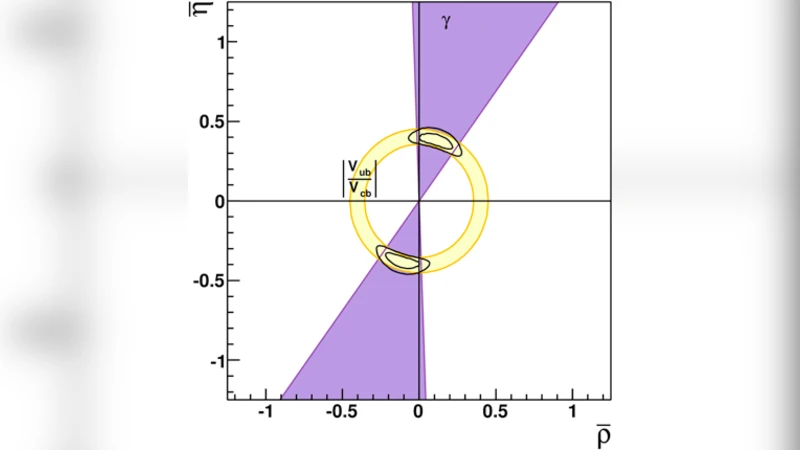
The authors illustrate the method with two concrete HEP problems. First, they consider the determination of the CKM parameters (\bar\rho) and (\bar\eta) (with fixed A and λ) from the measurement of the branching ratio (B\to\pi\ell\nu), which yields a reference posterior for (|V_{ub}|). Since all points satisfying (\bar\rho^2+\bar\eta^2=k) predict the same (|V_{ub}|), the LL domain is a circle of radius √k. The resulting 2‑D prior (\pi(\bar\rho,\bar\eta)=P(|V_{ub}|( \bar\rho^2+\bar\eta^2 ))/(2\pi(\bar\rho^2+\bar\eta^2))) is then used as the prior in a full CKM fit that also incorporates the measured CP‑violating phase γ. The allowed region obtained with this prior closely matches that obtained with a flat prior, but the reference‑based prior has a transparent statistical justification.

Second, they apply the framework to a simplified CMSSM (mSUGRA) model with parameters (m_0) and (m_{1/2}) (A₀=0, tanβ=10, μ>0). The observable is the expected signal yield (s(m_0,m_{1/2}) = \epsilon(m_0,m_{1/2}),\sigma(m_0,m_{1/2}),L), where ε is the selection efficiency, σ the production cross‑section, and L the integrated luminosity. The LL domain consists of all (m₀,m₁/₂) points that give the same s, which in practice form complex, non‑analytic iso‑yield contours. Computing the surface term K(m₀,m₁/₂) exactly is numerically demanding; the authors approximate it as a constant, justified by the near‑infinite length of the iso‑yield curves in the region of interest. Using a benchmark point (m₀=60 GeV, m₁/₂=250 GeV) they generate pseudo‑data for three luminosities (1 pb⁻¹, 100 pb⁻¹, 500 pb⁻¹) that exactly match the expectation. The resulting 2‑D priors display a pronounced peak at the true point, sharpening as the data sample grows, thereby demonstrating the consistency of the LL prescription.

In the conclusions, the authors emphasize that the reference‑prior‑based LL mapping provides a systematic, repeatable way to construct multi‑dimensional priors from well‑understood one‑dimensional measurements. Because reference priors possess good frequentist properties (e.g., asymptotic coverage), the resulting Bayesian analyses are expected to perform well even from a frequentist perspective. The main practical obstacle is the computation of the surface term K for realistic, high‑dimensional models; ongoing work aims to develop efficient numerical techniques for this purpose. Overall, the paper offers a pragmatic bridge between Bayesian rigor and the HEP community’s desire for objective, data‑driven inference, and it sets the stage for broader applications to more complex new‑physics scenarios.