Modelling Distributed Shape Priors by Gibbs Random Fields of Second Order

We analyse the potential of Gibbs Random Fields for shape prior modelling. We show that the expressive power of second order GRFs is already sufficient to express simple shapes and spatial relations between them simultaneously. This allows to model and recognise complex shapes as spatial compositions of simpler parts.

💡 Research Summary

The paper investigates how to use Gibbs Random Fields (GRFs) of second order as a compact yet expressive way to model shape priors for visual recognition. The authors start from the observation that human perception decomposes complex objects into simpler parts and interprets their spatial arrangement, a principle that should be exploited already in early stages of computer vision. Traditional global shape models (e.g., level‑set or variational approaches) treat a shape as a single continuous function and require a good initial pose; semi‑global models introduce auxiliary variables to capture local shape characteristics, but this leads to higher‑order potentials and increased computational complexity.

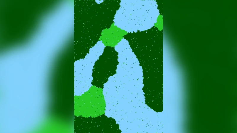
The central claim of the paper is that a second‑order GRF—i.e., a Markov random field whose cliques are all pairs of neighboring pixels defined by a set of displacement vectors A—already possesses enough expressive power to represent both simple shapes and the spatial relations between them. The model is defined on a finite pixel lattice D ⊂ ℤ². A set A ⊂ ℤ² specifies the allowed relative offsets; each offset a defines an equivalence class of edges Eₐ = {(t, t + a)}. For each a a potential function uₐ : K × K → ℝ is introduced, where K is the set of part labels plus a background label. All edges belonging to the same equivalence class share the same potential, which dramatically reduces the number of parameters while preserving translational invariance. The prior distribution over labelings y : D → K is

p(y) = (1/Z) exp