Considerate Approaches to Achieving Sufficiency for ABC model selection

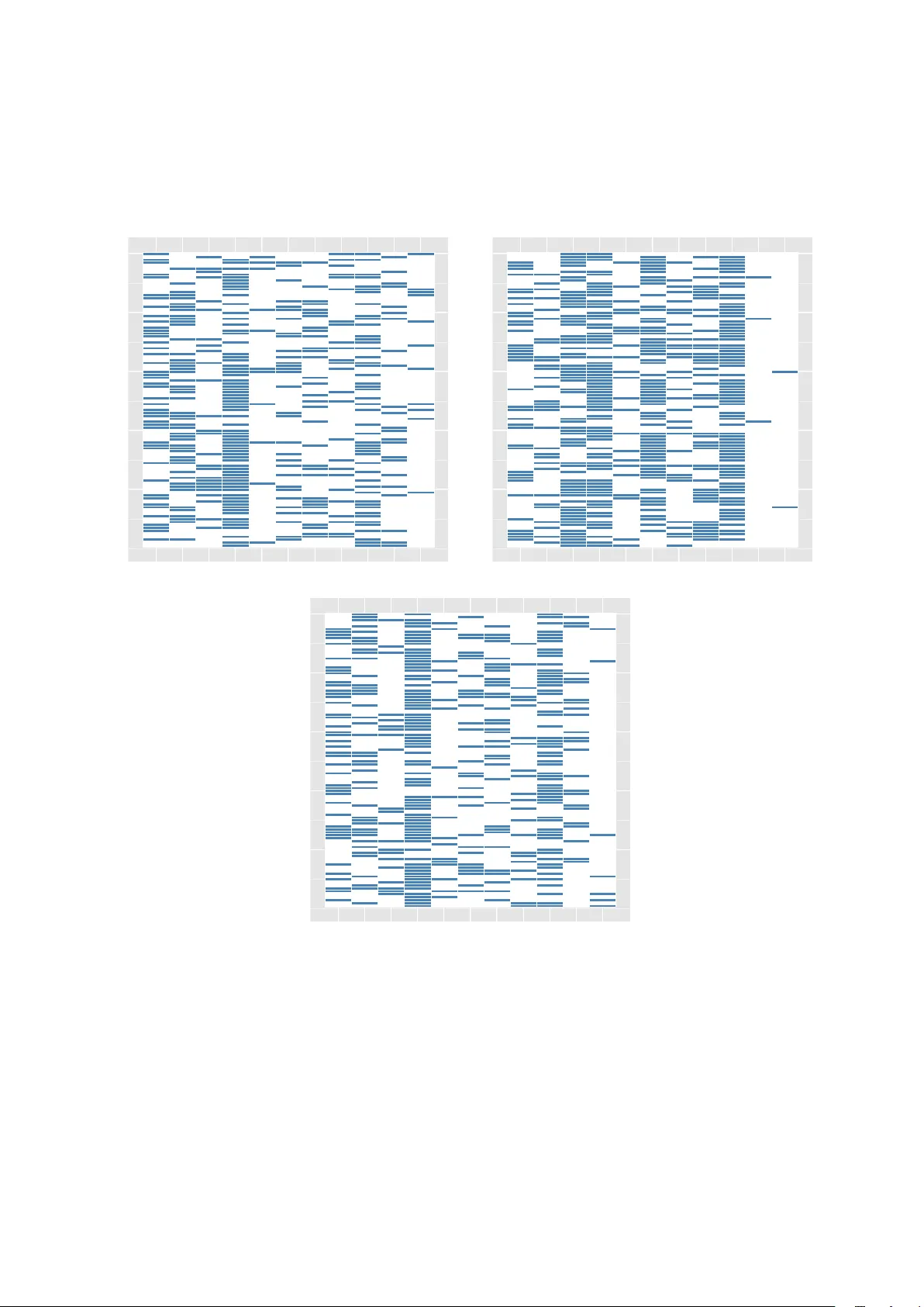
Considerate Approac hes to Ac hieving Sufficiency for ABC mo del selection Chris Barnes 1 , ∗ , Sarah Filippi 1 , ∗ , Mic hael P .H. Stumpf 1 , ∗ , # , Thomas Thorne 1 , ∗ 1 Cen tre for In tegrativ e Systems Biology and Bioinformatics, Imp erial College London, London SW7 2AZ, UK. Octob er 29, 2018 Abstract F or nearly an y challenging scientific problem ev aluation of the lik eliho o d is problematic if not imp ossible. Appro ximate Ba yesian computation (ABC) allows us to employ the whole Bay esian formalism to problems where w e can use sim ulations from a mo del, but cannot ev aluate the likeli- ho od directly . When summary statistics of real and simulated data are compared — rather than the data directly — information is lost, unless the summary statistics are sufficient. Here w e em- plo y an information-theoretical framew ork that can b e used to construct (approximately) sufficient statistics b y combining differen t statistics until the loss of information is minimized. Suc h sufficient sets of statistics are constructed for b oth parameter estimation and mo del selection problems. W e apply our approac h to a range of illustrative and real-world mo del selection problems. ∗ All authors con tributed equally . # T o Whom Corresp ondence Should be Addressed: m.stumpf@imp erial.ac.uk 1 In tro duction Mathematical models are widely used to describ e and analyze complex systems and pro cesses across the natural, engineering and so cial sciences. F orm ulating a mo del to describ e, e.g. a predator-prey system, geoph ysical pro cess, comm unication system, or social net work requires us to condense our assumptions and kno wledge into a single coherent framework (May, 2004). In constructing these mo dels we ha ve to state our assumptions ab out their constituent parts and their interactions explicitly . Mathematical analysis or computer simulations of these models then allows us to compare mo del predictions with exp erimental observ ations in order to test and ultimately improv e the mo dels. Even previously largely observ ational sciences suc h as biology , geology and meteorology are now heavily influenced by computer simulations which are employ ed for explanatory as well as predictiv e purp oses. Because man y of the mathematical models in these disciplines are to o complicated to b e analyzed in closed form, computer simulations ha ve become the primary tool in the theoretical analysis of very large or complex mo dels. Modelling such systems is often (relativ ely) straigh tforward if the mathematical structure of the mo del and reliable estimates for the model parameters are known. Unfortunately , it is considerably harder to infer the structure of mathematical mo dels and estimate their respective parameters based on experimental data, in particular if we seek to infer a mo del that can describe the data. Whenev er probabilistic mo dels exist we can emplo y standard mo del selection approaches of either a frequentist, Bay esian, or information theoretic nature (Co x & Hinkley, 1974; Mack ay, 2003; Burnham & Anderson, 2002). But if suitable probabilit y mo dels do not exist, or if the ev aluation of the likelihoo d is computationally in tractable, then we ha ve to base our assessmen t on the level of agreement b etw een simulated and observed data. This is particularly challenging when the parameters of sim ulation mo dels are not known but must b e inferred from observed data as well. F or such cases — cases where con v entional statistical approaches fail b ecause of the enormous computational burden incurred in ev aluating the likelihoo d — so-called approximate Bay esian computation (ABC) schemes ha ve recently come to the fore (Pritc hard et al. , 1999; Beaumont et al. , 2002; T anak a et al. , 2006; Secrier et al. , 1 2009). These forgo the explicit ev aluation of the lik eliho od b y a principled comparison betw een the observed and sim ulated data. In many cases inferences are furthermore based not on the data themselves, but on summary statistics of the data. Such statistics serve as data compression to ols(Cov er & Thomas, 2006) and, if used sensibly , enable computationally efficien t inference from data sets, where the complexity of the data would st ymie con ven tional lik eliho od-based metho ds (Pritchard et al. , 1999; Ratmann et al. , 2007). ABC schemes hav e b ecome increasingly popular, because of their flexibilit y and their deceptive conceptual simplicit y . While esp ecially some computationally demanding areas ha ve fuelled the developmen t of p o werful ABC approaches, notably p opulation genetics (F agundes et al. , 2007), evolutionary biology (Wilkinson et al. , 2010), systems biology (Liepe et al. , 2010), dynamical systems theory (T oni et al. , 2009), and epidemiology (Blum & T ran, 2008), a w orrying increase in naive (and plainly incorrect, see e.g. W alk er et al. (2010)) applications are b eginning to emerge. Suc h problems, as recent results by Didelot et al. (2010) and Rob ert et al. (2011) suggest, are more imminent in mo del selection applications. In the presen t context, all problems stem back to the issue of sufficiency of statistics, and its role in model selection. The presen t pap er sets out to develop remedies for suc h problems. Belo w w e will b egin with an outline of the basic ideas underlying ABC, before discussing the particular challenges raised in particular by Rob ert and colleagues. W e will then list the cases where ABC- based model selection is p ossible; in essence it is the ill-judged use of summary statistics and failure to ensure sufficiency which lies at the heart of the problem identified b y Robert et al. (2011), b efore setting out metho ds that allo w us to remedy these problems. W e illustrate the use of these methods in a n umber of applications b efore concluding with some more general remarks on the conceptual and mathematical foundations of ABC approac hes. 2 Appro ximate Ba y esian Computation 2.1 Sufficien t Statistics Ba yesian inference cen tres around the p osterior distribution , p ( θ | x ) = f ( x | θ ) π ( θ ) p ( x ) (1) where x are the data, whic h are drawn from some sample space, x ∈ Ω ⊆ R D , f ( x | θ ) is the likeliho o d , π ( θ ) the prior distribution , and θ an unknown parameter (Rob ert, 2007); p ( x ) is often called the evidence (Mack ay, 2003), but in many applications or discussions dismissed as a normalization constant. The Likeliho o d principle states that all the information about parameter θ is contained in the lik eliho o d function f ( x | θ ), i.e. once we ha ve the form of the lik eliho od, we do not ha ve to retain an y of the data. This principle is complemented by the sufficiency principle . Here a summary statistic of the general form S : R d − → R w , S ( x ) = s (2) with w  d t ypically , is called sufficient if the lik eliho od is independent of the parameter conditional on the v alue of the summary statistic. W e denote by f ( x | θ , s ) the likelihoo d conditionally on the v alue of the summary statistic S ( x ) = s and g ( x | s ) the densit y probability of the data given the summary statistic. The statistic is sufficien t if and only if: f ( x | s, θ ) = g ( x | s ) . The likelihoo d can then generally b e written in the Neyman-Fisher factorized form f ( x | θ ) = g ( x | s ) ˜ f ( s | θ ) , (3) where s = S ( x ) and ˜ f ( s | θ ) is the likelihoo d of the sufficient statistic (Cox, 2006). The function g ( · ) is indep endent of the parameter θ . Th us ˜ f ( s | θ ) carries all the information ab out the parameter. This factorization is, ho wev er, not unique, as it dep ends on the sufficient statistic, whic h is generally not unique. F or example, an y statistic containing additional information in addition to a sufficient statistic is also sufficien t. Therefore w e typically seek to determine the minimally sufficient statistic, which is generally unique. As a consequence the functional forms (and v alues) of g ( · ) and ˜ f ( ·| θ ) dep end on the c hoice of sufficien t statistics. In order to understand the terms in the factorization theorem, Eqn. (3), we fo cus on the case where X is a discrete random v ariable, we then hav e g ( x | s ) = Pr( X = x |S ( X ) = s ) 2 and ˜ f ( s | θ ) = Pr( S ( X ) = s | θ ) . Th us g ( x | s ) is really the conditional probability of X giv en an observed v alue for the summary statistic, S ( X ) = s and it is therefore link ed to the compression of the data achiev ed b y the summary statistic. Here it is w orth remem b ering that the complete data also form a v alid summary statistic, and for this choice of statistic w e hav e trivially , for all s , g ( x | s ) = 1 , ∀ x ∈ Ω. 2.2 ABC for parameter inference In practical applications we are in terested in ev aluating the p osterior distribution for mo del parameters, θ , defined Eqn. (1). When the likelihoo d is hard to ev aluate it is still often possible to sim ulate from the mo del according to f ( ·| θ ). It is easy to show that for simulated data y w e ha ve p ( θ | x ) = 1 ( x = y ) f ( y | θ ) π ( θ ) p ( x ) , (4) whic h in man y practical applications can b e approximated using suitable distance functions, ∆( x, y ), whence, after marginalization o ver simulated data we get, p ( θ | x ) ≈ Z Ω 1 (∆( x, y ) ≤  ) f ( y | θ ) π ( θ ) p ( x ) dy . (5) This is ob viously correct, as  − → 0. Based on the fact that sufficient statistics con tain all the information ab out the θ that is contained in the data, we may be tempted to replace the data by the corresp onding summary statistics. W e th us replace the comparison of the data in Eqn. (5) by a comparison of the v alues of their respective summary statistics, using a distance function which, by abusing the notation, is denoted b y ∆( S ( x ) , S ( y )), p ( θ | x ) ≈ Z Ω 1 (∆( S ( x ) , S ( y )) ≤  ) f ( y | θ ) π ( θ ) p ( x ) dy = R R D 1 (∆( S ( x ) , s ) ≤  ) ˜ f ( s | θ ) π ( θ ) ds R Θ R R w 1 (∆( S ( x ) , s ) ≤  ) ˜ f ( s | θ ) π ( θ ) dsdθ , (6) where we hav e made it explicit in the second line that once we use summary statistics we are only considering the second term on the right-hand side of Eqn. (3); any dep endence on g ( · ) is lost, and so is therefore the effect of the data-compression in the summary statistic. Something similar is also implicit in con v entional Bay esian inference. Cox (2006) reinforces this point b y stating that “ Any Bayesian infer enc e uses the data only via the minimal sufficient statistic. This is b e c ause the c alculation of the p osterior distribution involves multiplying the likeliho o d by the prior and normalizing. Any factor of the likeliho o d that is a function of y alone wil l disapp e ar after normalization. ” Quite generally , the choice of the summary statistic is imp ortan t: without sufficiency the whole inference will only map the parameter regimes that will lead to mo del b eha viour which embo dies the constrain ts implied b y sp ecified summary statistic. Only if the summary statistic is sufficient, how ever, will w e b e able to infer the mo del parameters (F earnhead & Prangle, 2010a). F or some non-sufficien t statistics, ho wev er, some asp ects of the true p osterior can be elucidated as sho wn in Figure 1. W e will return to a discussion of non-sufficien t statistics later. 2.3 ABC for mo del selection One of the p erhaps most useful (and aesthetically pleasing) asp ects of the Bay esian inferen tial framew orks is that mo del selection is natural and intrinsic, esp ecially compared to frequentist framew orks (Rob ert, 2007). F rom the earliest days ABC approac hes for mo del selection ha ve also b een promoted, see e.g. Beaumon t et al. (2002) and F agundes et al. (2007). Recently , how ev er, Rob ert et al. (2011) hav e issued a note of caution. This is based on the observ ation that a statistic, or set of statistics, whic h is sufficien t for mo del parameters in different mo dels, may still not be sufficient across mo dels (Didelot et al. , 2010; Rob ert et al. , 2011). 3 θ p ( θ ) 0 200 400 600 0 50 100 150 200 250 mean −4 −2 0 2 4 min −4 −2 0 2 4 0 5 10 15 20 25 30 0 50 100 150 200 250 300 var −4 −2 0 2 4 max −4 −2 0 2 4 Figure 1: Parameter inference for the mean of a normal model with kno wn standard deviation, σ 2 = 1, using the mean, v ariance, maximum and minim um as a statistic. W e find that only the truly sufficient statistic ( θ = µ = 1) yields the correct p osterior distribution despite the fact that w e generated 1,000 acceptances of samples of size 10,000 with  = 0 . 001. 4 T o illustrate this p oint we now consider a finite set of mo dels, M = { M 1 , . . . , M q } , eac h of which has an asso ciated parameter v ector θ m ∈ Θ m , 1 ≤ m ≤ q . W e aim to p erform inference on the joint sp ac e ov er mo dels and parameters, ( m, θ m ). Rob ert et al. (2011) ha ve focused on the Bay es F actors, but, of course, similar problems arise also for the marginal mo del likelihoo ds, p ( m | x ) = R Θ m f ( x | θ m ) π ( θ m ) dθ m π ( m ) P q i =1 R Θ i f ( x | θ i ) π ( θ i ) dθ i π ( i ) . (7) Again, we can apply ABC b y replacing ev aluation of the likelihoo d in fav our of comparing simulated and real data for differen t parameters drawn from the p osterior, whence w e obtain p ( m | x ) ≈ R Θ m R Ω 1 (∆( x, y ) ≤  ) f ( y | θ m ) π ( θ m ) dθ m dy π ( m ) P q i =1 R Θ i R Ω 1 (∆( x, y ) ≤  ) f ( y | θ i ) π ( θ i ) dθ i dy π ( i ) , (8) whic h is of course alwa ys exact once  − → 0. The same is no longer true, how ever, once the complete data hav e b een replaced by summary statistics. So in general p ( m | x ) 6 = R Θ m R R w 1 (∆( S m ( x ) , s m ≤  ) ˜ f ( s m | θ m ) π ( θ m ) dθ m ds m π ( m ) P q i =1 R Θ i R R w 1 (∆( S i ( x ) , s i ) ≤  ) ˜ f ( s i | θ i ) π ( θ i ) dθ i ds i π ( i ) ; , (9) where S i , 1 ≤ i ≤ q are the summary statistics for eac h mo del. An equality can only hold if the factors g i ( x ) , 1 ≤ i ≤ q are all identical. Otherwise the differen t levels of data-compression are lost and un biased mo del selection is no longer p ossible. 2.4 Resuscitating ABC Mo del Selection As shown by Robert et al. (2011) and Didelot et al. (2010) ev en if w e choose a set of statistics that is sufficient for parameter estimation across models, this do es not guaran tee that the same set of statistics are sufficient for mo del selection. R Robert et al. (2011) argue that therefore model selection, though not parameter estimation is fraught with problems in an ABC framew ork. Here we will argue that this is not the case. While we do agree that sufficiency and problems when using inadequate (or insufficient ) statistics for mo del selection, we main tain that • this mirrors problems that can also b e observ ed in the parameter estimation context (see Figure 1), • for man y imp ortant, and arguably the most imp ortant applications of ABC, this problem can in principle b e av oided by using the whole data rather than summary statistics, • in cases where summary statistics are required, we argue that we can construct approximately sufficient statistics in a disciplined manner, • when all else fails, a c hange in p erspective, allo ws us to nevertheless make use of the flexibility of the ABC framework (see Discussion). The bulk of this article will deal with the deriv ation and application of a metho d that constructs summary statistics appropriate for the twin use of parameter estimation and mo del selection. After this w e will briefly return to an outline of alternativ e approac hes and map the applicability of ABC-based mo del selection more generally . 3 Some Basic Concepts from Information Theory Our metho d is most easily framed in the terms of information theory (Mac k ay, 2003; Co ver & Thomas, 2006; M ´ ezard & Montanari, 2009), and in order to keep this article self-con tained we briefly review some of the basic concepts. W e let X denote a discrete random v ariable with p otential states X and probability mass function p X ( x ) = Pr ( X = x ), x ∈ X . In this section, for sake of clarity , we explicitly denote the random v ariables as subscript of the corresp onding probability density . 5 3.1 En trop y and Mutual Information The entr opy of X , denoted by H , measures the uncertain ty of X and is defined as follows, H ( X ) = − X x p X ( x ) log p X ( x ) = − E X [log p X ( X )] = E X  1 log p X ( X )  ≥ 0 , where E X denotes the exp ectation under the probabilit y mass function p X . Let ( X , Y ) b e a pair of discrete random v ariables with joint distribution p X,Y . The c onditional entr opy H ( Y | X ) is defined as H ( Y | X ) = − E X,Y  log p Y | X ( Y | X )  . The mutual information I ( X ; Y ) b et w een tw o discrete random v ariables X and Y measures the amount of information that Y contains ab out X . It can be seen as the reduction of the uncertaint y ab out X due to the kno wledge of Y , I ( X ; Y ) = H ( X ) − H ( X | Y ) = X x,y ∈X p X,Y ( x, y ) log p X,Y ( x, y ) p X ( x ) p Y ( y ) = K L ( p X,Y || p X p Y ) ≥ 0 , where K L ( P || Q ) refers to the Kul lb ack-L eibler (KL) div ergence b et ween probabilities P and Q . The mutual information I ( X ; Y ) is equal to 0 if and only if the random v ariables X and Y are indep endent. The c onditional mutual information of discrete random v ariables X , Y and Z is defined as I ( X ; Y | Z ) = H ( X | Z ) − H ( X | Y , Z ); it is the reduction in uncertaint y of X due to knowledge of Y when Z is giv en. This quantit y is zero if and only if X and Y are conditionally indep enden t giv en Z , which means that Z contains all the information ab out X in Y . The conditional mutual information satisfies the chain rule: for discrete random v ariables X 1 , X 2 , · · · , X n and Y we hav e I ( X 1 , X 2 , · · · , X n ; Y ) = n X i =1 I ( X i ; Y | X 1 , X 2 , · · · , X i − 2 , X i − 1 ) . In the following we only consider en tropy , rather than the differen tial entrop y , which applies to contin uous random v ariables. 3.2 Data Pro cessing Inequality and Sufficien t Statistics The data pr o c essing ine quality (DPE) states that for random v ariables X , Y , and Z such that X → Y → Z , (i.e. Y dep ends, deterministically or randomly , on X and Z dep ends on Y ) I ( X ; Y ) ≥ I ( X ; Z ) , with equalit y only if X → Y → Z forms a Marko v Chain, which means that the random v ariables X and Z are conditionally indep endent giv en Y : p X,Z | Y = p X | Y p Z | Y . No w consider a family of distributions { f ( ·| θ ) } θ ∈ Θ and let X be a sample from a distribution in this family . Let S b e a deterministic statistic and denote b y S the random v ariable such that S = S ( X ). Therefore θ → X → S . By the DPE I ( θ ; S ) ≤ I ( θ ; X ) . Analogously to the discussion ab o ve, a statistic S is said sufficient for p ar ameter θ if and only if S contains all the information in X ab out θ , i.e. I ( θ ; S ) = I ( θ ; X ) where S = S ( X ) Equiv alen tly w e may write: Result 1. S is a sufficient statistic for p ar ameter θ if and only if I ( θ ; X | S ) = 0 . In that c ase, E θ,X  log p ( θ | X ) p ( θ | S )  = 0 . 6 F rom now on, we resume the use of typically bay esian notation (see section 2) where the random v ariables are no longer given as subscripts but are unambiguously inferred from context. F or example, the density of probability p ( θ | S ) inv olved in the theorem designates b oth the p osterior probability of the parameter θ conditional on S and its v alue when the parameter is actually equal to θ . Pr o of. By definition, S is a sufficien t statistic if and only if I ( θ ; X ) = I ( θ ; S ). S b eing a deterministic fonction of X , the previous equation is equiv alen t to I ( θ ; X , S ) − I ( θ ; S ) = 0 ⇔ H ( θ ) − H ( θ | X, S ) − H ( θ ) + H ( θ | S ) = 0 ⇔ H ( θ | S ) − H ( θ | X, S ) = 0 ⇔ I ( θ ; X | S ) = 0 If S is a sufficient statistic for parameter θ then I ( θ ; X ) = I ( θ ; S ) ⇔ X θ,x p ( θ , x ) log p ( θ , x ) p ( θ ) p ( x ) = X θ,s p ( θ , s ) log p ( θ , s ) p ( θ ) p ( s ) ⇔ X θ,x p ( θ , x ) log p ( θ , x ) p ( θ ) p ( x ) = X θ,x p ( θ , x ) log p ( θ , S ( x )) p ( θ ) p ( S ( x )) ⇔ X θ,x p ( θ , x ) log p ( θ , x ) p ( θ ) p ( S ( x )) p ( θ ) p ( x ) p ( θ, S ( x )) = 0 ⇔ X θ,x p ( θ , x ) log p ( θ | x ) p ( θ |S ( x )) = 0 4 Constructing Sufficien t Statistics W e consider the following situation: supp ose that w e hav e a finite set of summary statistics S = {S 1 , . . . , S w } and assume that S is a sufficien t statistic. W e aim to identify a subset U of S which is sufficien t for θ . The follo wing result characterizes such a subset. Result 2. L et S b e a finite set of summary statistics of X , and assume that S is a sufficient statistic. Denote by U a subset of S . F or a r andom variable X distribute d ac c or ding to a distribution p ar ametrize d by θ , let U = U ( X ) and S = S ( X ) . The fol lowing statements hold U is a sufficient statistic ⇔ I ( θ ; S | U ) = 0 ⇔ E X [ K L ( p ( θ | S ) || p ( θ | U ))] = 0 . Pr o of. By definition of the conditional m utual information I ( θ ; S | U ) = H ( θ | U ) − H ( θ | S, U ) = H ( θ ) − H ( θ | S, U ) − H ( θ ) + H ( θ | U ) = I ( θ ; U, S ) − I ( θ ; U ) = I ( θ ; S ) − I ( θ ; U ) since U is a vector composed of elemen ts of S . The statistic S being sufficien t, I ( θ ; S ) = I ( θ ; X ), and therefore I ( θ ; S | U ) = 0 if and only if U is a sufficient statistic. Denote by h the function suc h that for all x , u = U ( x ) = 7 h ( S ( x )), I ( θ ; S | U ) = H ( θ | U ) − H ( θ | S, U ) = X θ,s,u p ( θ , s, u ) log  p ( θ | u, s ) p ( θ | u )  = X θ,s p ( θ , s ) log  p ( θ | h ( s ) , s ) p ( θ | h ( s ))  = X θ,s p ( θ , s ) log  p ( θ | s ) p ( θ | h ( s ))  = X s p ( s ) X θ p ( θ | s ) log  p ( θ | s ) p ( θ | h ( s ))  = X s p ( s ) K L ( p ( θ | s ) || p ( θ | h ( s ))) = X x p ( x ) K L ( p ( θ |S ( x )) || p ( θ |U ( x ))) = E X [ K L ( p ( θ | S ) || p ( θ | U ))] . According to this result identifying a sufficien t statistic with minimum cardinalit y from a sufficient family S of summary statistics b oils down to identifying the smallest subset U of S such that I ( θ ; S | U ) = 0 where U = U ( X ) and S = S ( X ) or, equiv alently , E X [ K L ( p ( θ | S ) || p ( θ | U ))] = 0. Here w e aim to determine a sufficient statistic for Appro ximate Ba yesian Computation (ABC) metho ds for parameter inference and then for mo del selection. W e focus in this section on the parameter inference task. In the ABC framework, the exp ectation o v er the data of the Kullbac k-Leibler div ergence (Cov er & Thomas, 2006) betw een the tw o p osterior distributions p ( θ | S ) and p ( θ | U ) cannot b e exactly computed since w e only hav e at our disp osal a dataset x and the v alue of the statistics for this dataset s ∗ = ( s ∗ 1 , . . . , s ∗ w ) = S ( x ). Thus, w e approximate it by the exp ectation with resp ect to the empirical measure of the data. The metho d is summarized in Algorithm 1. W e denote by | U | the cardinalit y of a set U . Algorithm 1 Minimization of the mutual information 1: input: a sufficient set of statistics whose v alues on the dataset is s ∗ = { s ∗ 1 , . . . , s ∗ w } 2: output: a subset U ∗ of s ∗ 3: for all u ∗ ⊂ s ∗ do 4: p erform ABC to obtain ˆ p ( θ | u ∗ ) 5: end for 6: let T ∗ = { u ∗ ⊂ s ∗ suc h that K L ( ˆ p ( θ | s ∗ ) || ˆ p ( θ | u ∗ )) = 0 } 7: return U ∗ = argmin u ∗ ∈ T ∗ | u ∗ | This methodology is computationally prohibitive since it en umerates all p ossible subsets u ∗ of s ∗ and perform the ABC algorithm for all of these. Moreov er, it is challenging to obtain a precise estimate of the p osterior ˆ p ( θ | u ∗ ) of θ given a v alue of the statistics U = u ∗ when the cardinalit y of u ∗ is large. In particular, it is often imp ossible to obtain an estimate of p ( θ | s ∗ ). It is then necessary to design an algorithm whic h do es not need the computation of this probability . The following result pro vides a first step into this direction. Result 3. L et X b e a r andom variable gener ate d ac c or ding to f ( ·| θ ) . L et S b e a sufficient statistic and U and T two subsets of S such that U = U ( X ) , T = T ( X ) and S = S ( X ) satisfy U ⊂ T ⊂ S . We have I ( θ ; S | T ) = I ( θ ; S | U ) − I ( θ ; T | U ) . Pr o of. F or all subset T of S , I ( θ ; S | T ) = H ( θ | T ) − H ( θ | S, T ) = H ( θ | T ) − H ( θ | S ) . Then, for U and T subsets of S , I ( θ ; S | T ) − I ( θ ; S | U ) = H ( θ | T ) − H ( θ | U ) . If U in included in T , then H ( θ | T ) = H ( θ | T , U ) and I ( θ ; S | T ) − I ( θ ; S | U ) = − I ( θ ; T | U ) whic h pro ves the result. 8 It follows that the information con tained in S on θ giv en T is smaller than the information contained in S on θ given U ⊂ T . In order to construct a subset T of S such that I ( θ ; S | T ) = 0, where S = S ( X ) and T = T ( X ), it is th us sufficien t to add one by one statistics of S un til the condition holds. Indeed, if we denote the statistic added at time step k ≤ w by S ( k ) and S ( k ) = S ( k ) ( X ), then I ( θ ; S | S (1) , . . . , S ( k ) ) ≤ I ( θ ; S | S (1) , . . . , S ( k +1) ) . And there exists an integer k ≤ w suc h that I ( θ ; S | S (1) , . . . , S ( k ) ) = 0. According to result 3, at each time k , I ( θ ; S | S (1) , . . . , S ( k ) ) = I ( θ ; S | S (1) , . . . , S ( k − 1) ) − I ( θ ; S (1) , . . . , S ( k ) | S (1) , . . . , S ( k − 1) ) . The mutual information is a non negative function, then, in order to decrease as muc h as p ossible I ( θ ; S | S (1) , . . . , S ( k ) ), the added statistic at time k > 1 should b e such that S ( k ) = argmax V ∈ S \{ S (1) ,...,S ( k − 1) } I ( θ ; S (1) , . . . , S ( k − 1) , V | S (1) , . . . , S ( k − 1) ) = argmax V ∈ S \{ S (1) ,...,S ( k − 1) } E X  K L  p ( θ | S (1) , . . . , S ( k − 1) , V ) || p ( θ | S (1) , . . . , S ( k − 1) )  . As previously mentioned, in practice, this exp ectation can not b e computed. W e hence replace it by the exp ectation with resp ect to the empirical measure of the data, leading to the approximation, for all 1 ≤ k ≤ n , argmax V ∈ S \{ S (1) ,...,S ( k − 1) } E p ( X )  K L  p ( θ | S (1) , . . . , S ( k − 1) , V ) || p ( θ | S (1) , . . . , S ( k − 1) )  ≈ argmax v ∗ ∈ s ∗ \{ s ∗ (1) ,...,s ∗ ( k − 1) } K L  p ( θ | s ∗ (1) , . . . , s ∗ ( k − 1) , v ∗ ) || p ( θ | s ∗ (1) , . . . , s ∗ ( k − 1) )  , where s ∗ is the v alue of the statistic S on the dataset. In addition, the first statistic S (1) should con tain the maxim um information ab out θ , in the sense that S (1) = argmax V ∈ S I ( θ ; V ) = argmin V ∈ S H ( θ | V ) = argmax V ∈ S E p ( θ,V ) [log p ( θ | V )] . This results in algorithm 2. Algorithm 2 Greedy minimization of the m utual information 1: input: a sufficient set of deterministic statistics whose v alues on the dataset is s ∗ = { s ∗ 1 , . . . , s ∗ w } 2: output: a subset U ∗ of s ∗ 3: for all u ∗ ∈ s ∗ , p erform ABC to obtain ˆ p ( θ | u ∗ ) 4: let s ∗ (1) = argmax u ∗ ∈ s ∗ log ˆ p ( θ | u ∗ ) 5: for k ∈ { 2 , . . . , w } do 6: for all u ∗ ∈ s ∗ \ n s ∗ (1) , . . . , s ∗ ( k − 1) o , p erform ABC to obtain ˆ p ( θ | s ∗ (1) , . . . , s ∗ ( k − 1) , u ∗ ) 7: let s ∗ ( k ) = argmax u ∗ K L ( ˆ p ( θ | s ∗ (1) , . . . , s ∗ ( k − 1) , u ∗ ) || ˆ p ( θ | s ∗ (1) , . . . , s ∗ ( k − 1) )) (10) 8: if K L ( ˆ p ( θ | s ∗ (1) , . . . , s ∗ ( k ) ) || ˆ p ( θ | s ∗ (1) , . . . , s ∗ ( k − 1) )) ≤  then 9: return U ∗ = ( s ∗ (1) , . . . , s ∗ ( k − 1) )) 10: end if 11: end for 12: return U ∗ = s ∗ This algorithm is computationally expensive if the cardinalit y of the set of statistics |S | = w is large. Indeed at each iteration k , one p erforms the ABC algorithm w − k + 1 times. A simplification of it consists in replacing the maximization step (see equation (10)) by testing randomly v arious statistics and choosing a statistic S ( k ) suc h that I ( θ ; S (1) , . . . , S ( k ) | S (1) , . . . , S ( k − 1) ) is large. Different criteria may be used to determine if the m utual information is large or not, and then decide if the statistic should b e included or not. Most of these criteria consist of determining if the posterior probability of θ given S (1) , . . . , S ( k − 1) and the posterior probability of θ given S (1) , . . . , S ( k ) are significan tly differen t. If so, adding the statistic S ( k ) is justified, otherwise w e do not add it and instead turn to a different statistic. In the algorithm 3, we denote by C h p ( θ | s ∗ (1) , . . . , s ∗ ( k ) ) , p ( θ | s ∗ (1) , . . . , s ∗ ( k − 1) ) i the criterion which is equal to 1 if the statistic S ( k ) should be added and 0 otherwise. In practice, w e can use, for instance, one of the following measures: 9 • w e add the statistic S ( k ) if K L ( p ( θ | s ∗ (1) , . . . , s ∗ ( k ) ) || p ( θ | s ∗ (1) , . . . , s ∗ ( k − 1) )) ≥ δ k where δ k is a threshold which ma y b e computed by b o otstrapping the data to estimate E p ( X )  p ( θ | S (1) , . . . , S ( k − 1) )  : δ k = K L  p ( θ | s ∗ (1) , . . . , s ∗ ( k ) ) || E p ( X )  p ( θ | S (1) , . . . , S ( k − 1) )   , • the Kolmogorov-Smirno v test enables us to compare p ( θ | s ∗ (1) , . . . , s ∗ ( k − 1) ) and p ( θ | s ∗ (1) , . . . , s ∗ ( k ) ) and so, the statistic S ( k ) is added if the test has a p -v alue smaller than a certain threshold, say 0 . 01. Algorithm 3 Sto c hastic minimization of the m utual information 1: input: a sufficient set of deterministic statistics whose v alues on the dataset is s ∗ = { s ∗ 1 , . . . , s ∗ w } 2: output: a subset V ∗ of s ∗ 3: c ho ose randomly u ∗ in s ∗ 4: T ∗ ← s ∗ \ { u ∗ } 5: V ∗ ← u ∗ 6: rep eat 7: rep eat 8: if T ∗ = Ø then return V ∗ 9: end if 10: c ho ose randomly u ∗ in T ∗ 11: T ∗ ← T ∗ \ u ∗ 12: p erform ABC to obtain ˆ p ( θ | V ∗ , u ∗ ) 13: un til C [ ˆ p ( θ | V ∗ , u ∗ ) , ˆ p ( θ | V ∗ )] = 1 14: T ∗ ← s ∗ \ { V ∗ , u ∗ } 15: optional ly: V ∗ ← Or derDep endency ( V ∗ , u ∗ ) and T ∗ ← s ∗ \ V ∗ 16: V ∗ ← V ∗ ∪ u ∗ 17: un til T ∗ = Ø 18: return V ∗ The order in which the statistics are added matters (Jo yce & Marjoram, 2008; Nunes & Balding, 2010) and the only wa y to a void this incon venience is to use the computationally exp ensiv e algorithm 2. Nevertheless, w e suggest to test for order dep endency before deciding on whether to add a statistic. This consists of determining if, giv en the recently added statistic u ∗ , the previously added statistics in V ∗ still bring relev ant information or are not necessary anymore and hence ma y b e released from the set under construction. More precisely , after line 15 of the algorithm 3, we add the function describ ed in algorithm 4. Algorithm 4 Order Dep endency 1: Input: A set of accepted statistics V ∗ = { s ∗ (1) , . . . , s ∗ ( k − 1) } and the last accepted statistic u ∗ 2: Output: A subset U ∗ of { V ∗ ∪ u ∗ } 3: U ∗ ← u ∗ 4: for i ∈ { 1 , . . . , k − 1 } do 5: if C ( p ( θ | U ∗ , s ∗ ( i ) ) , p ( θ | U ∗ )) = 1 then 6: U ∗ ← U ∗ ∪ s ∗ ( i ) 7: end if 8: end for 9: return U ∗ 5 Relation to previous work The presented information theoretic framework builds up on tw o previous methods for summary statistic selec- tion. Our main contributions are the generalisation of the notion of approximate sufficiency , rigorous deriv ations 10 of algorithms using information theory and the application of summ ary statistic selection for the joint space. Jo yce & Marjoram (2008) developed a notion of appro ximate sufficiency for parameter inference and pre- sen ted a sequential algorithm to score statistics according to whether their inclusion w ould impro ve the inference. Their sequential algorithm resembles (and indeed inspired) Algorithm 3 although they do not retain statistics once they ha ve failed to b e added whic h w e feel is required since whether a statistic is added dep ends strongly on the statistics already accepted. Their rule for adding statistics is essen tially an approximate test for inde- p endence on the p osterior distribution under the addition of a new statistic but can only b e used for single parameter mo dels. W e hav e shown that the true stopping criterion should b e the change in KL div ergence whic h can b e used for multiv ariate p osteriors, although tests for indep endence (KS, χ 2 ) can b e used as an appro ximation in single parameter mo dels. Nunes & Balding (2010) prop osed a heuristic algorithm to minimize the entrop y of the p osterior with resp ect to sets of summary statistics . Additionally they prop osed a refinemen t step where the set of statistics that minimised the posterior mean root sum of squared errors (MRSSE) w as selected. The minim um entrop y approac h is related to Algorithm 1 since, when H ( θ ) is constant, minimising the en tropy maximises the m utual information. Ho wev er, assuming there exists a sufficient statistic, choosing the set of statistics that minimises the en tropy is guaran teed to give sufficiency but not minimal sufficiency since adding a statistic to a sufficien t set can reduce the entrop y by chance (a manifestation of “conditioning alw ays reduces en tropy”). 6 Automated selection of summary statistics for mo del selection As p oin ted out recently sufficiency across models is still not sufficien t to p erform reliably mo del choice in the ABC framework. Here we sho w how a natural extension of the metho dology in tro duced ab o ve can also b e emplo yed in order to construct sets of statistics that are sufficient for ABC-based mo del selection, when it is impractical to use the raw data (T oni & Stumpf, 2010). Consider q mo dels, eac h with an as sociated set of parameters Θ i , i ∈ { 1 , ..., q } . W e aim to identify a set of sufficien t statistic for model selection. Let M b eing a random v ariable taking v alue in { 1 , . . . , q } . A statistic is sufficien t for mo del selection if and only if it is sufficient for the joint space { M , { θ i } 1 ≤ i ≤ q } . According to result 1, this means that a summary statistic S is sufficien t for mo del selection if and only if I ( M , θ 1 , ...., θ q ; X | S ) = 0 where S = S ( X ) and X is a sample from a distribution in the family { f ( ·| θ i ) } θ i ∈ Θ i , 1 ≤ i ≤ q . The following result enables us to link this condition with the sufficiency for parameter inference for eac h model. Result 4. F or al l deterministic statistic S , I ( M , θ 1 , ...., θ q ; X | S ) = I ( M ; X | θ 1 , ...., θ q , S ) + X i I ( θ i ; X | S ) , wher e S = S ( X ) and X is a sample fr om a distribution in the family { f ( ·| θ i ) } θ i ∈ Θ i , 1 ≤ i ≤ q . Pr o of. F rom the chain rule of mutual information we hav e that I ( M , θ 1 , ...., θ q ; X | S ) = I ( M ; X | θ 1 , ...., θ q , S ) + X i I ( θ i ; X | θ 1 , · · · , θ i − 1 , S ) . The result then follows from the fact that, for all i , I ( θ i ; X | θ 1 , · · · , θ i − 1 , S ) = I ( θ i ; X | S ). The mutual information b eing alwa ys non negative, this shows that a statistic S is sufficient for mo del selection if and only if I ( M ; X | θ 1 , ...., θ q , S ) = 0 and I ( θ i ; X | S ) = 0 for all i ∈ { 1 , · · · , q } . Therefore, a sufficien t statistic for model selection is sufficien t for parameter inference in each model and, given the parameter v alues for every models, the statistic is sufficien t for inferring the model. Thus, in order to identify a sufficient statistic for model selection, one should determine a set of minimal sufficien t statistics S m i for eac h mo del 1 ≤ i ≤ q and then identify among all statistics T containing ∪ i ∈{ 1 ··· q } S m i the one with the smallest cardinality suc h that I ( M ; X | θ 1 , ...., θ q , T ) = 0. The method, summarized in algorithm 5, consists in running one of the previous algorithms, for example algorithm 3 and then add statistics whic h bring new information ab out the mo dels in the sense that the p osterior probabilit y of the model conditional on the statistics v aries significantly if we add a this new statistic. Similarly to algorithm 3, it is p ossible to test for order dependency b efore deciding to add a statistic. T o do so, we apply the algorithm 4 in which at step 3, the set U ∗ is initialized by M ∗ ∪ u ∗ suc h that w e alw ays k eep the set M ∗ and condition line 5 is replaced by C h ˆ p ( M | θ 1 , . . . , θ q , U ∗ , s ∗ ( i ) ) , ˆ p ( M | θ 1 , . . . , θ q , U ∗ ) i = 1. 11 Algorithm 5 Sto c hastic minimization of the m utual information for mo del selection 1: input: a sufficient set of deterministic statistics whose v alues on the dataset is s ∗ = { s ∗ 1 , . . . , s ∗ w } 2: output: a subset V ∗ of s ∗ whic h is sufficien t for mo del selection 3: for i ∈ { 1 , . . . , q } do 4: determine a sufficien t statistic whose v alue on the dataset is S m i ⊂ s ∗ using algorithm 3 5: end for 6: Let M ∗ = ∪ 1 ≤ i ≤ q S m i 7: Let W ∗ ← s ∗ \ M ∗ 8: c ho ose randomly u ∗ in W ∗ 9: T ∗ ← W ∗ \ { u ∗ } 10: V ∗ ← u ∗ 11: rep eat 12: rep eat 13: if T ∗ = Ø then return V ∗ 14: end if 15: c ho ose randomly u ∗ in T ∗ 16: T ∗ ← T ∗ \ u ∗ 17: p erform ABC to obtain ˆ p ( M | θ 1 , . . . , θ q , M ∗ , V ∗ , u ∗ ) 18: un til C [ ˆ p ( M | θ 1 , . . . , θ q , M ∗ , V ∗ , u ∗ ) , ˆ p ( M | θ 1 , . . . , θ q , M ∗ , V ∗ )] = 1 19: T ∗ ← W ∗ \ { V ∗ , u ∗ } 20: optional ly: V ∗ ← Or derDep endenc eMo delSele c ( V ∗ , M ∗ ∪ u ∗ ) and T ∗ ← W ∗ \ V ∗ 21: V ∗ ← V ∗ ∪ u ∗ 22: un til T ∗ = Ø 23: return V ∗ 7 Applications W e illustrate the framework dev elop ed ab ov e in three differen t contexts. First we consider a simple mo del selection problem in volving tw o normal distributions. W e then consider a t ypical p opulation genetics example on three demographic scenarios for simulated data, b efore finally turning to a problem where we consider alternativ e random walk mo dels; this last example should b e t ypical for applications where likelihoo d-based inferences are out of the question due to the complexit y of the models and the data. 7.1 Normal example The developed framew ork w as illustrated on a simple example with tw o mo dels y 1 , ...y d ∼ N ( µ, σ 2 1 ) and y 1 , ...y d ∼ N ( µ, σ 2 2 ) , where the v ariances of the normal distributions, σ 1 and σ 2 , are fixed. Under a conjugate prior, µ ∼ N (0 , a 2 ), the true Ba yes factor is given by B F ( y ) = σ − d 1 exp {− S 2 / 2 σ 2 1 } exp {− ¯ y 2 / 2( a 2 + σ 2 1 /d ) } q a − 2 + dσ − 2 2 σ − d 2 exp {− S 2 / 2 σ 2 2 } exp {− ¯ y 2 / 2( a 2 + σ 2 2 /d ) } q a − 2 + dσ − 2 1 , where ¯ y = d − 1 d X i =1 y i and S 2 = d X i =1 ( y i − ¯ y ) 2 . In this case ¯ y is sufficient for parameter inference but the pair { ¯ y , S 2 } is sufficien t for the joint space. T o test the automated choice of appro ximate summary statistics, 100 data sets were sampled under mo del 1 and the algorithm run to select statistics for parameter inference and for the join t space from a po ol of 5 12 statistics including ¯ y , S 2 , range, maximum and a non informative statistic u ∼ U (0 , 2). The v alues of the parameters were chosen to b e σ 1 = 0 . 3, σ 2 = 0 . 6, n = 15 and a = 2. Since there are difficulties that arise from the p ossibly very different scales of the summary statistics the distance w as defined as ∆( S ( x ) , S ( y )) = X i [log S i ( x ) − log S i ( y )] 2 , whic h accoun ts for the relativ e difference betw een data and sim ulation and av oids the need to known the scales of the statistics a priori . Here, S i ( x ) denotes the i -th comp onen t of S ( x ) ∈ R w The stopping criteria w ere defined through tests for indep endence ( p < 1 × 10 − 5 ) betw een the p osterior distributions under differen t summary statistics; a Kolmogorov-Smirno v test in the case of the contin uous parameter p osterior and a P earson test in the case of the discrete mo del posterior. The ABC was run with 500 particles with  = 0 . 1. Figure 2 sho ws the results of the summary statistic selection ov er the 100 runs. Figure 2 (left) sho ws the results for parameter inference across the t wo mo dels. The mean w as selected in ev ery replicate, the maximum in 14 replicates and S 2 once. Figure 2 (righ t) sho ws the additional statistics selected for the join t space. S 2 w as selected in 84 cases, the range in 19 cases, the maximum in 9 cases and the noise statistic once. Figure 3 shows the Bay es F actor obtained via ABC versus the analytical prediction. As exp ected the Bay es factor calculated using only the statistics selected for parameter inference is uncorrelated with the true Ba yes factor (figure on the left). When the statistics sufficien t for the joint space are included the ABC Ba yes factor correlates well with the analytical prediction. 7.2 P opulation genetics example T o further demonstrate the efficacy of our methodology w e applied the summary statistic selection pro cedure to a real world ABC problem, that of mo del selection in p opulation genetics. Data were generated using coalescen t sim ulations (Hudson, 1991) from three competing mo dels, producing 100 data sets from eac h for fixed parameters using a mo dified version of the MS softw are pack age do wnloadable from http://home.uchicago. edu/rhudson1/source/mksamples.html ). The mo dels considered were: Mo del 1 Constant population size (with population mutation rate θ = 20, corresp onding to a 20,000bp stretc h of DNA in a p opulation of size N = 1 , 000 , 000. Mo del 2 Exp onen tial gro wth mo del with exp onential gro wth rate γ = 0 . 4 and all other parameters as ab o ve. Mo del 3 Two island model with scaled migration rate m = 10 and all other parameters as ab o ve. T o p erform ABC we generated 5 , 000 , 000 samples of datasets comprising 100 c hromosomes for each mo del; in each case the population mutation rate θ (Ewens, 2004) w as dra wn from the prior U (5 , 30); the real v alue for whic h the data were generated was θ = 20 (measured in units of total p opulation size). The summary statistics summarised b elow w ere then used in our ABC summary statistic selection framew ork to derive sufficien t sets of summary statistics for mo del selection on the observ ed data. The summary statistics calculated were: S1 Num b er of Segregating Sites, N S . S2 Num b er of Distinct Haplotypes, N H . S3 Homozygosit y , h H , where h is the probability that t wo haplotypes are identical, h H = N H X h =1 ν 2 h . S4 Av erage SNP Homozygosity , ¯ h S = N S X i =1 ( ν 0 ( i ) 2 + ν 1 ( i ) 2 ) . S5 Num b er of occurences of most common haplot yp e, f H . S6 Mean num b er of pair-wise differences betw een haplot yp es, T . 13 Run 20 40 60 80 100 mean S2 range max random Run 20 40 60 80 100 mean S2 range max random Figure 2: Summary statistics selected in 100 runs of the automated summary statistic selection. Left: Statistics selected for parameter inference (the union of statistics found under model 1 and model 2). Righ t: Additional statistics chosen for the joint space. ● ● ● ● ● ● ● ● ● ● ● ● ● ● ● ● ● ● ● ● ● ● ● ● ● ● ● ● ● ● ● ● ● ● ● ● ● ● ● ● ● ● ● ● ● ● ● ● ● ● ● ● ● ● ● ● ● ● ● ● ● ● ● ● ● ● ● ● ● ● ● ● ● ● ● ● ● ● ● ● ● ● ● ● ● ● ● ● ● ● ● ● ● ● ● ● ● ● ● ● −2 0 2 4 6 8 −2 0 2 4 6 log(BF) predicted log(BF) ABC ● ● ● ● ● ● ● ● ● ● ● ● ● ● ● ● ● ● ● ● ● ● ● ● ● ● ● ● ● ● ● ● ● ● ● ● ● ● ● ● ● ● ● ● ● ● ● ● ● ● ● ● ● ● ● ● ● ● ● ● ● ● ● ● ● ● ● ● ● ● ● ● ● ● ● ● ● ● ● ● ● ● ● ● ● ● ● ● ● ● ● ● ● ● ● ● ● ● ● ● −2 0 2 4 6 8 −2 0 2 4 6 8 log(BF) predicted log(BF) ABC Figure 3: Predicted vs appro ximated log Bay es F actor for the normal to y model. Left: The case for sufficien t statistics selected for parameter inference. Righ t: The case for sufficien t statistics selected for the join t space. In b oth cases the red line represents the line y = x . 14 S7 Num b er of Singleton Haplotypes, f sH S8 Num b er of Singleton SNPs, f sS . S9 Link age Disequilibrium measured by r 2 = 2 N S ( N S − 1) N S − 1 X i =1 N S X j = i +1 ( ν 00 ( i, j ) − ν 0 ( i ) ν 0 ( j )) 2 ν 0 ( i ) ν 1 ( i ) ν 0 ( j ) ν 1 ( j ) S10 F raction of pairs of lo ci which violate the four-gamete test, i.e. for which the t wo-locus haplotypes 00, 01, 10 and 11 exist. S11 Random v ariable, ρ ∼ U [0 , 1] . where N is the num b er of sequences in the data, and for eac h SNP lo cus, i , let ν 0 ( i ) ν 1 ( i ) denote the frequencies of the ancestral and derived alleles; further for any haplotype h , ν h is the corresp onding frequency . The results of the selection pro cess when p erformed ov er 100 different simulated data sets from each of the three mo dels considered are shown in figure 4. It is apparent that the c hosen statistics v ary b et ween data sets generated quite considerably — this is to b e exp ected as the statistics required for sufficiency will v ary dep ending on the data. F or data generated by all of the mo dels it is apparent that S4 , the av erage SNP homozygosit y , is selected often, whilst as exp ected the uninformative random statistic S11 is rarely chosen. F or data generated under the exponential growth model, S4 , as well as S3 (homozygosity), S6 (mean num b er of pair-wise differences b et ween haplot yp es) and S9 (link age disequilibrium), appear to b e fa voured by the mo del selection approach. Data generated from this mo del apparently requires more statistics than data generated from the Null model to ac hieve sufficiency . The metho d applied to data generated from the tw o island mo del selects statistics S4 and S9 often, in terestingly seeming to require fewer statistics than the exponential growth mo del to p erform model selection. This is a new and initially perhaps surpising finding: the summaries chosen b y our model selection approach dep end subtly on the true data-generating mo del. This is, b y hindsight, ho wev er, not unexp ected: we are trying to achiev e sufficiency for model parameters first, and then p o ol the statistics required to do just that for all mo dels, before refining this set of statistics in order to obtain sufficiency for mo del selection. As some mo dels will generate data that is more difficult to obtain under other mo dels than is the case vice v ersa, such relative biases will affect the set of statistics c hosen. In light of p opulation genetics theory , therefore, our observ ations are completely in line with our understanding of coalescent pro cesses (see e.g. Hein et al. (2005)). 7.3 Random w alk mo dels W e also apply our framework to the problem of mo del selection on random walks, using a n umber of summary statistics. The mo dels (Rudnick & Gaspari, 2010) under consideration were: Mo del 1 Brownian motion. Mo del 2 Persisten t random walk (where the walk is more lik ely to con tinue in the same direction ov er successive steps but do es not hav e a particular fa voured orientation). Mo del 3 Biased random walk (where one direction is fav oured). W e used fiv e summary statistics, that are individually not sufficien t in more than one dimension for an y of the random w alk mo dels: S1 Mean square displacemen t. S2 Mean x and y displacemen t. S3 Mean square x and y displacement. S4 Straigh tness index. S5 Eigen v alues of gyration tensor (reference random walks bo ok). 15 Run 20 40 60 80 100 S1 S2 S3 S4 S5 S6 S7 S8 S9 S10 S11 Run 20 40 60 80 100 S1 S2 S3 S4 S5 S6 S7 S8 S9 S10 S11 Run 20 40 60 80 100 S1 S2 S3 S4 S5 S6 S7 S8 S9 S10 S11 Figure 4: Summary statistics selected in 100 runs of the automated summary statistic selection pro cedure on sim ulated data se ts from our three p opulation genetics mo dels. (eac h run is p erformed on a differen t simulated observed data p oint). A) Statistics chosen for mo del selection with data generated from model 1. B) Statistics chosen for mo del selection with data generated from mo del 2. C) Statistics c hosen for model selection with data generated from mo del 3. 16 Since the mo dels ha ve m ultiple parameters, we can no longer apply a χ 2 test to select sufficient statistics, and so instead w e approximate the KL-div ergence using the p osterior, applying the formula describ ed in (Boltz et al. , 2007), K L ( p X || p Y ) ≈ log N V N U − 1 + d E U [log ρ k ( · , V )] − d E U [log ρ k ( · , U )] , (11) where U and V are the sets of p osterior particles drawn from distributions p X and p Y resp ectiv ely , d is the n umber of parameters and E U [log ρ k ( · , V )] is the expectation of the distance to the k th nearest neighbour in the set of particles V , ρ k ( u, V ) of each particle u ∈ U . Applying formula (11) in our summary statistic selection framew ork to data simulated from the three differen t mo dels ov er 100 runs, the statistics shown in figure 5 are chosen. Again it is apparen t that there are some differences in the selected statistics for different data sets generated. Lo oking at the summary statistics selected by our metho d, statistic S5 , the eigenv alues of the gyration tensor, a measure of the anisotrop y of the random w alk, app ears to b e c hosen often for data generated b y all three mo dels. There also app ears to be a sligh t preference for statistic S2 , the mean x and y displacemen t, whic h can be understo o d given that this statistic is necessary for sufficiency for parameter inference on the biased random w alk mo del. W e need to stress that the structure of the data here is complex and summary statistics are expected to b e h ugely v ariable. 8 Discussion Sufficien t statistics are rare; in conv enient form — i.e. where the n umber of statistics is equal to the n umber of parameters to b e estimated — they are restricted to problems that can be describ ed in terms of mo dels that b elong to the exp onential family (Lehmann & Casella, 1993; Didelot et al. , 2010). As previous authors hav e p oin ted out it is necessary to develop metho ds that construct sets of statistics that are (at least approximately (Le Cam, 1964; Kusama, 1976)) sufficient (Jo yce & Marjoram, 2008; Nunes & Balding, 2010; F earnhead & Prangle, 2010a,b). It is either this, or rein terpreting ABC-based inferences not as appro ximations to the full Ba yesian (and thus lik eliho o d-based) apparatus but as inference pro cedures in their o wn right (Wilkinson, 2008; Dro v andi et al. , 2011), p otentially systematically biased or for appro ximate mo dels. A third approach, previously adv o cated, is to consider mo del c hecking rather than model selection as a viable wa y of ensuring that only appropriate mo dels are calibrated against data. W e b eliev e that the latter p osition fails to ac knowledge the role of sufficiency of statistics also in the context of parameter estimation; and we will briefly return to this p oin t b elow after having addressed the other t wo p oin ts. All methods aimed at constructing collections of statistics that tak en together are (appro ximately) sufficien t will fail, almost trivially , unless an exhaustive set of summary statistics can b e envisioned which fulfils the sufficiency criteria as outlined abov e. If that is not the case, then w e might naively exp ect that all candidate summary statistics from our starting set S will b e included in U . This, how ever, need not (and we b eliev e generally will not) be the case, as the information theoretical framework will tend to bias against inclusion of statistics that are in some w ay co-linear to an y statistics that are already included in the constructed set. It is, of course, in principle possible to use the KL div ergence with resp ect to the distribution obtained with the full data as an ov erall b enc hmark, but in cases where this is indeed p ossible, it may b e b est to use the full data (see e.g. T oni et al. (2009)) for inference rather than risk the information reduction inherent to most summary statistics. There has b een m uch interest in trying to interpret ABC not solely as an approximation to the “true” p osterior, but as an inferential framework in its own right (Wilkinson, 2008; Drov andi et al. , 2011). This is p erhaps an attractiv e option. One wa y of achieving this shift in p erspective is to consider distributions such as p ( M , θ | S ) as distributions whic h sp ecify the probability of a parameter and mo del b eing in concordance with a given summary statistic. If all w e care ab out is that a model and parameter combination hav e high (or lo w) probability of pro ducing data with certain mean/maxim um/minimum or an y other summary statistic v alue, then this is p erfect. It is easy to envisage scenarios where we are only interested in certain aspects of the data (such as maxim um w ater levels). ABC metho ds can b e used to infer parameters (and models) that are more lik ely to giv e rise to simulated data that shares some but not all characteristics of the data. In terestingly , this w ould also allow us to emplo y ABC as a design to ol (Barnes et al. , 2011): we sp ecify the data (or system behaviour) 17 Run 20 40 60 80 100 S1 S2 S3 S4 S5 Run 20 40 60 80 100 S1 S2 S3 S4 S5 Run 20 40 60 80 100 S1 S2 S3 S4 S5 Figure 5: Summary statistics selected in 100 runs of the automated summary statistic selection on differen t simulated data sets, considering three different random walk mo dels. A) Statistics chosen for mo del selection with data generated from mo del 1. B) Statistics c hosen for mo del selection with data generated from model 2. C) Statistics chosen for mo del selection with data generated from mo del 3. 18 that we w ould lik e to observe and infer parameters (and mo dels) whic h hav e high probability of producing these t yp es of b eha viour. While this may p erhaps seem lik e sophistry it do es also hav e serious implications for mo del c hecking: any ABC approach that is based on summary statistics will infer mo del parameters (or marginal mo del p osteriors) that reflect the b eha viour enco ded b y these statistics. Thus w e can no longer use these same statistics for model c hecking. This reflects the need to use non-sufficient summary statistics for mo del chec king from Bay esian p osterior predictiv e distributions: if w e p erform inference under a mo del for which a sufficient statistic exists, then calculating the same statistic for replicate data generated from the p osterior predictiv e distribution will result in test statistics that are in line with the observed data, irresp ectiv e of the v alidit y of the mo del. Hence some authors, in particular Gelman et al. (2003), strongly advocate the use of graphical model c hec king tech- niques o ver numerical tests. W e feel that the situation in ABC reflects some of the same problems that are also encoun tered in mo del c hecking. Th us in an ABC framework, irresp ectiv e of whether the statistics are sufficien t or not, the p osterior distributions reflect the c hoice of statistics and the same statistics are therefore ill-suited for mo del chec king. W e conclude by reiterating that ABC approaches employing summary statistics rather than the whole data hav e to fully engage with the level of information-loss inherent to summary statistics. Notions of simple sufficien t statistics probably do not apply for most scien tifically in teresting and c hallenging problems and the use of statistics rather than the real data will alw a ys result in loss of information. Our approac h is based around the assessmen t of information loss and allo ws the principled construction of sets of statistics (from a candidate set) that capture as m uch as possible from the observed data. While not a panacea, it is within the computational reac h of ABC practitioners and makes information loss due to inadequate use of statistics apparent, for b oth the parameter and mo del selection problems. References Barnes, C., Silk, D., Sheng, X. & Stumpf, M. 2011 Bay esian design of syn thetic biological systems ARXIV q-bio.MN, stat.AP , 1103.1046. Beaumon t, M., Zhang, W. & Balding, D. 2002 Approximate Ba yesian computation in p opulation genetics Genetics 162 , 2025–2035. Blum, M. G. B. & T ran, V. C. 2008 HIV with con tact-tracing: a case study in Approximate Ba yesian Compu- tation ARXIV stat.AP published in: Biostatistics 11, 4 (2010) 644-660. Boltz, S., Debreuve, E. & Barlaud, M. 2007 Eigh th In ternational W orkshop on Image Analysis for Multimedia In teractive Services (WIAMIS ’07) in Eighth International Workshop on Image A nalysis for Multime dia Inter active Servic es (WIAMIS ’07) 16–16 IEEE. Burnham, K. & Anderson, D. 2002 Mo del selection and m ultimo del inference: A practical information-theoretic approac h Springer Scienc e+Business Me dia, Inc. . Co ver, T. & Thomas, J. 2006 Elements of Information The ory Wiley-Interscience. Co x, D. 2006 Principles of Statistic al Infer enc e Cambridge: Cambridge Universit y Press. Co x, D. & Hinkley , D. 1974 The or etic al Statistics New Y ork: Chapman&Hall/CRC. Didelot, X., Everitt, R., Johansen, A. & Lawson, D. 2010 Lik eliho o d-free estimation of mo del evidence war- wick.ac.uk . Dro v andi, C. C., Pettitt, A. N. & F addy , M. J. 2011 Appro ximate Ba yesian computation using indirect inference Journal of the R oyal Statistic al So ciety Series C-Applie d Statistics 60 , 317–337. Ew ens, W. 2004 Mathematic al Population Genetics 2nd edition New Y ork: Springer. F agundes, N. J. R., Ray , N., Beaumont, M., Neuensc hw ander, S. et al. 2007 Statistical ev aluation of alternative mo dels of human evolution. Pr o c Natl A c ad Sci U S A 104 , 17614–17619. 19 F earnhead, P . & Prangle, D. 2010a Constructing Summary Statistics for Approximate Bay esian Computa- tion: Semi-automatic ABC arXiv.or g stat.ME v2: Revised in resp onse to reviewer comments, adding more examples and a metho d for inference from multiple data sources. F earnhead, P . & Prangle, D. 2010b Semi-automatic Appro ximate Ba yesian Computation ARXIV stat.ME . Gelman, A., J.B., C., Stern, H. & Rubin, D. 2003 Bayesian Data Analysis 2nd edition Chapman & Hall/CRC. Hein, J., Sc hierup, M. & Wiuf, C. 2005 Gene Gene alo gies, variation and evolution Oxford Univ ersity Press. Hudson, R. R. 1991 Gene genealogies and the coalescent pro cess. Jo yce, P . & Marjoram, P . 2008 Approximately Sufficien t Statistics and Ba yesian Computation Statistic al Ap- plic ations in Genetics and Mole cular Biolo gy Lo ok up nearly sufficient statistics. Kusama, T. 1976 On approximate sufficiency Osaka Journal of Mathematics 13 , 661–669. Le Cam, L. 1964 Sufficiency and Appro ximate Sufficiency The A nnals of Mathematic al Statistics 35 , 1419–1455. Lehmann, E. & Casella, G. 1993 The ory of p oint estimation Springer. Liep e, J., Barnes, C., Cule, E., Erguler, K. et al. 2010 ABC-SysBio–approximate Bay esian computation in Python with GPU supp ort. Bioinformatics (Oxfor d, England) 26 , 1797–1799. Mac k ay , D. J. 2003 Information the ory, infer enc e and le arning algorithms Cambridge Universit y Press. Ma y , R. M. 2004 Uses and abuses of mathematics in biology Scienc e 303 , 790–3 doi:10.1126/science.1094442. M ´ ezard, M. & Montanari, A. 2009 Information, Physics and Computation Oxford Univ ersity Press. Nunes, M. A. & Balding, D. J. 2010 On Optimal Selection of Summary Statistics for Approximate Ba yesian Computation Statistic al Applic ations in Genetics and Mole cular Biolo gy 9 . Pritc hard, J. K., Seielstad, M. T., Perez-Lezaun, A. & F eldman, M. W. 1999 Population growth of human Y c hromosomes: a study of Y chromosome microsatellites Mol Biol Evol 16 , 1791–1798. Ratmann, O., Jorgensen, O., Hinkley , T., Stumpf, M., Richardson, S. & Wiuf, C. 2007 Using likelihoo d-free inference to compare evolutionary dynamics of the protein net works of H. p ylori and P . falciparum. PL oS Computational Biolo gy 3 , e230. Rob ert, C. 2007 The Bayesian Choic e Springer. Rob ert, C. P ., Cornuet, J.-M., Marin, J.-M. & Pillai, N. 2011 Lac k of confidence in ABC model choice stat.ME 8 pages, 7 figures, 1 table, submitted to the Pro ceedings of the National Academ y of Sciences, extension of Rudnic k, J. & Gaspari, G. 2010 Elements of the R andom Walk Cambridge Universit y Press. Secrier, M., T oni, T. & Stumpf, M. P . H. 2009 The ABC of rev erse engineering biological signalling systems. Mole cular Biosystems 5 , 1925–1935. T anak a, M. M., F rancis, A. R., Luciani, F. & Sisson, S. A. 2006 Using approximate bay esian computation to estimate tub erculosis transmission parameters from genotype data. Genetics 173 , 1511–1520 doi:10.1534/ genetics.106.055574. T oni, T. & Stumpf, M. P . H. 2010 Simulation-based mo del selection for dynamical systems in systems and p opulation biology Bioinformatics 26 , 104–110. T oni, T., W elch, D., Strelko wa, N., Ipsen, A. & Stumpf, M. P . 2009 Appro ximate Bay esian computation scheme for parameter inference and mo del selection in dynamical systems Journal of the R oyal So ciety, Interfac e / the R oyal So ciety 6 , 187–202. 20 W alk er, D. M., Allingham, D., Lee , H. W. J. & Small, M. 2010 Parameter inference in small world netw ork dis- ease models with approximate Bay esian Computational metho ds PHYSICA A-ST A TISTICAL MECHANICS AND ITS APPLICA TIONS 389 , 540–548. Wilkinson, R. D. 2008 Approximate Bay esian computation (ABC) giv es exact results under the assumption of mo del error ARXIV stat.CO 13 pages, 1 figure. Wilkinson, R. D., Steip er, M. E., Soligo, C., Martin, R. D., Y ang, Z. & T a v ar ´ e, S. 2010 Dating Primate Div ergences through an In tegrated Analysis of P alaeontological and Molecular Data Systematic Biolo gy . 21