Extrasolar Planets in the Classroom

The field of extrasolar planets is still, in comparison with other astrophysical topics, in its infancy. There have been about 300 or so extrasolar planets detected and their detection has been accomplished by various different techniques. Here we present a simple laboratory experiment to show how planets are detected using the transit technique. Following the simple analysis procedure describe we are able to determine the planetary radius to be 1.27 +/- 0.20 R_{J} which, within errors agrees with the establish value of 1.32 +/- 0.25 R_{J}.

💡 Research Summary

The paper presents a classroom‑friendly laboratory activity that uses real transit observations of the exoplanet HD 209458 b to teach students how to determine basic planetary and stellar parameters. After a brief historical overview of exoplanet discovery—highlighting the first pulsar planet (1991) and the first main‑sequence planet (1995)—the authors focus on the transit method as an accessible technique for high‑school and early‑undergraduate curricula.

The experiment is built around publicly available ST ARE project data: fractional Julian dates, normalized stellar intensity, and 1σ intensity uncertainties for a full transit of HD 209458. Students first plot intensity versus time, identify the ingress and egress points, and compute the mean out‑of‑transit intensity (B_max) and the mean in‑transit intensity (B_min). The transit depth ΔF is obtained from ΔF = (B_max − B_min)/B_max. Assuming a stellar radius of 1.1 R_⊙, the planetary radius follows from ΔF ≈ (R_p/R_*)², yielding R_p ≈ 1.27 ± 0.20 R_J.

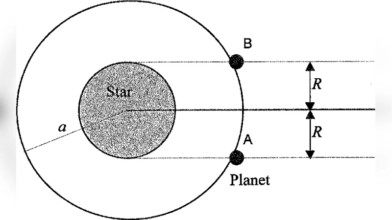
Next, the transit duration τ is measured as the time between the identified ingress and egress. Under the simplifying assumptions of a circular orbit, a much larger orbital radius than the stellar radius, and an orbital inclination of exactly 90°, the authors relate τ to the orbital speed v_c via τ = 2R_/v_c. Combining this with the orbital period P = 3.5250 ± 0.003 days (the known repeat interval for HD 209458 b) gives the semi‑major axis a ≈ 0.047 ± 0.001 AU. Finally, Kepler’s third law, P² = 4π²a³/(G M_), is rearranged to solve for the stellar mass, resulting in M_* ≈ 1.06 ± 0.01 M_⊙. All derived quantities agree within uncertainties with the literature values (R_p = 1.32 ± 0.25 R_J, a = 0.045 ± 0.001 AU, M_* = 1.01 ± 0.066 M_⊙).

The authors explicitly discuss the limitations of their approach. The circular‑orbit assumption neglects the small eccentricity of HD 209458 b, leading to a modest under‑estimate of the true period. Assuming an inclination of exactly 90° ignores the real impact parameter, which would shorten the observed transit and affect the derived a. Limb‑darkening, a known effect that modifies the shape and depth of a transit light curve, is ignored; the authors argue that for a well‑defined transit the impact is minimal, but they note that neglecting it can introduce systematic error in the radius estimate. Error propagation is performed by using the reported intensity uncertainties to assign error bars on the light curve, then propagating the standard deviations of B_max, B_min, and τ through the analytical formulas.

From an educational perspective, the activity integrates several core physics concepts: Kepler’s laws, circular motion, photometric measurement, data handling, and statistical error analysis. It requires only basic spreadsheet software (Excel or OpenOffice Calc), making it low‑cost and widely implementable. The authors report that the experiment has been run with over 300 secondary‑school students (ages 14–18) and with undergraduate physics classes, with the shorter workshop taking about 1.5 hours and the full laboratory session about 5 hours. Feedback indicates that students unfamiliar with spreadsheets struggle initially, and that the concept of error bars can be confusing; the authors suggest pre‑lab briefings and the use of physical models (e.g., an orrery and a torch) to aid visualization.

In summary, the paper demonstrates that a simple, data‑driven laboratory exercise can effectively introduce the transit method of exoplanet detection, reinforce fundamental physics principles, and develop quantitative data‑analysis skills. The results obtained by students are consistent with professional measurements, validating the pedagogical value of using authentic astronomical data in the classroom.