Quadratic choreographies

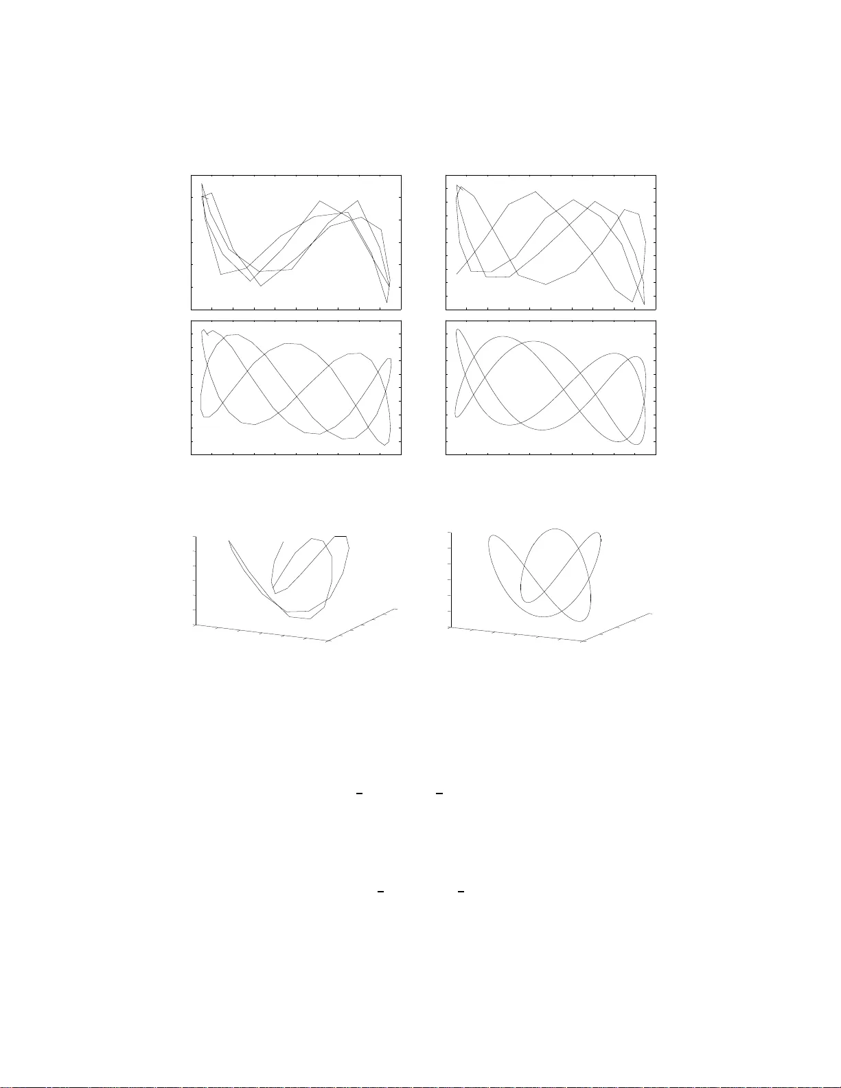
Quadrat ic c horeog raphies P . Ryck elynck a, , L. Smo ch a a ULCO, LMP A, F -62100 Calais, F r anc e Univ Lil le Nor d de F r anc e, F-59000 Lil le, F r anc e . CNRS, FR 2956, F r anc e. Abstract This pa p er addresses the classical and discrete Euler-La grange equations for systems o f n pa rticles interacting quadra tically in R d . By highlig hting the r ole play ed by the center of mass of the particle s , we solve the pr evious systems via the classical quadratic eigenv alue problem (QEP ) and its discr ete transcendental generaliza tion. The ro ots of class ical and discrete QEP being giv en, we state some conditional conv ergence results. Next, we fo cus esp ecia lly on p erio dic and c horeog raphic solutions and w e provide s ome numerical expe r iment s whic h confirm the co n vergence. Keywor ds: Calculus of v ariations , F unctional equations, Discretiza tion, Quadratic eigenv alue pr oblems, Perio dic and almost-p erio dic solutions 2000 MSC: 49 K21, 49K15, 65L0 3, 6 5L12 1. In tro duction This pap er s e eks to co n tinue the developmen t of the theory for the disc r ete calculus of v ariations which was initiated by Cres son and al., see [2, 3]. It consists originally in r eplacing the de r iv a tive ˙ x ( t ) of the dy namic v a riable x ( t ) defined on [ t 0 , t f ] with a 2 N + 1 terms scale der iv a tive  ε x ( t ) = N X j = − N γ j ε x ( t + j ε ) χ − j ( t ) , t ∈ [ t 0 , t f ] , γ j ∈ C (1) where χ j ( t ) denotes the characteristic function of [ t 0 , t f ] ∩ [ t 0 + j ε, t f + j ε ], for some time delay ε . W e co nsider a lagra ngian L of n particles in R d , where d denotes the “phys- ical” dimension. The principle of leas t action may b e extended to the cas e of non-differentiable dynamic v ar iables. F or conserv ative sy s tems, the equations of motion may b e returned a s the following t wo dyna mic sets of equa tions ¨ x j ( t ) = F j ( x 1 , . . . , x n ) and −  − ε  ε x j ( t ) = ˜ F j ( x 1 , . . . , x n ) (2) Email addr esses: ryckelyn@lmp a.univ-littoral.fr (P . Ryck elync k), smoch@lm pa.univ-litt oral.fr (L. Smo ch ) Pr eprint submitted to Elsevier Octob er 20, 2018 where the functions F j , ˜ F j are built fro m the specific in teraction b et ween the particles. While the fir st system in (2) deals with ODE, the second one cons ists in a set of functional difference equations . W e investigate for eac h sys tem the existence of ps eudo-p erio dic solutions of the shap e u ( t ) = u 0 + K X ℓ =1 e λ ℓ t u ℓ , (3) where u 0 and u ℓ constitute a family of K + 1 vectors of C d and ( λ ℓ ) ℓ ∈ ( C ⋆ ) K is a sequence o f K distinct co mplex num ber s. The rest of this pap er is orga nized a s follo ws. Sec tio n 2 is dev oted to the deriv ation of the clas s ical and discr ete Euler-Lagrang e e quations (resp ectively abbreviated as C.E.L. and D.E.L.) and highlights the role play ed b y the center of mass 1 n x s ( t ) where x s ( t ) = P j x j ( t ). In Section 3, we present a method for s olving the equations of motio n for g eneric la grangia ns for C.E.L. as w ell as D.E.L.. The first step o f this metho d determines x s ( t ) from some generalized (quadratic or transcendental) eigenv alue pro blem. The second step seeks x j ( t ) from x s ( t ) by solving a nother eig env alue problem. Section 4 is devoted to the conv ergence of the g eneralized eig env alue pr oblem linked to the D.E.L. as ε tends to 0. Section 5 deals with the existence a nd the featur es of p erio dic and choreographic solutions . Finally , Section 6 presen ts some numerical exper iment s illustrating the phenomenon of conv ergence as ε tends to 0, for some v ar ious op erators  ε . 2. Equations o f m otion for symm etric quadr atic lagrangians of n par- ticles systems in R d The pr inciple o f least discrete action has b een de velop ed in [7, 8] to which we refer throughout the pap er. W e denote by C pw the space of the functions x : [ t 0 , t f ] → R d contin uous on eac h in terv al [ t 0 + j ε, t 0 + ( j + 1 ) ε ] ∩ [ t 0 , t f ] for all j ≥ 0 and small enough, i.e. j ≤ t f − t 0 ε . If X = ( x 1 , . . . x n ) deno tes a sy s tem of n functions in C pw , w e ma y think of X as the set of dynamic v a riables describing the state of a system of n interacting particles in R d . W e consider actions A cont , A disc : C n pw → R of the shap e A cont ( X ) = Z t f t 0 L ( X ( t ) , ˙ X ( t )) dt, A disc ( X ) = Z t f t 0 L ( X ( t ) ,  ε X ( t )) dt. (4) F r om now on, w e drop t from the for m ulas when it is clea r enough. W e intro duce a general quadratic lagrangian o f n par ticles in R d , compatible with discr ete s ymmetries of the sy stem. Let J 1 , . . . , J 5 ∈ C 0 ([ t 0 , t f ] , R d × d ), J 1 , . . . , J 4 be symmetric matrices and J 6 , J 7 ∈ C 0 ([ t 0 , t f ] , R d ). F o r an iso lated particle with p ositio n x and velo city y we may set L 1 ( x , y ) = 1 2 t y J 1 y + 1 2 t x J 2 x + t x J 5 y + t J 6 y + t J 7 x . 2 Next, tw o particles with p ositions x j , x k , and v eloc ities y j , y k are interacting for pairs in co nformity with the following lagra ngian L 2 ( x j , y j , x k , y k ) = t y j J 3 y k + t x j J 4 x k . Therefore, the lag rangian of the who le system is L = n X j =1 L 1 ( x j , ˙ x j ) + X j 6 = k L 2 ( x j , ˙ x j , x k , ˙ x k ) . (5) The or em 2.1 . L et X = ( x 1 , . . . , x n ) in C n pw and x s = n X j =1 x j . A ne c essary and sufficient c ondition for X to b e a critic al p oint of A cont in C n pw is that X satisfies the dynamic syst em ( J 1 − 2 J 3 ) ¨ x j + ( − 2 ˙ J 3 + t J 5 + ˙ J 1 − J 5 ) ˙ x j + ( t ˙ J 5 − J 2 + 2 J 4 ) x j = − 2 J 3 ¨ x s − 2 ˙ J 3 ˙ x s + 2 J 4 x s + ( J 7 − ˙ J 6 ) , ∀ j. (6) A ne c essary and sufficient c ondition for X to b e a critic al p oint of A disc in C n pw is that X satisfies the line ar functional r e curr enc e system of e quations  − ε (( J 1 − 2 J 3 )  ε x j ) +  − ε ( t J 5 x j ) + J 5  ε x j + ( J 2 − 2 J 4 ) x j = − 2  − ε ( J 3  ε x s ) − 2 J 4 x s − (  − ε J 6 + J 7 )) , ∀ j. (7) Pr o of. W e first reca ll the classical and discrete Euler-Lagr ange equations, whic h are resp ectively given by − d dt ∂ L ∂ ˙ x j ( t, X ( t ) , ˙ X ( t )) + ∂ L ∂ x j ( t, X ( t ) , ˙ X ( t )) = 0 (8) and  − ε ∂ L ∂  ε x j ( t, X ( t ) ,  ε X ( t )) + ∂ L ∂ x j ( t, X ( t ) ,  ε X ( t )) = 0 , (9) for all j ∈ { 1 , . . . , n } . The computation o f gradients of L needs the following prop erty : if a , b ∈ R d , ∇ x ( t ax + t xb ) = a + b . Let us prove (6). Beca use of the symmetry of J 1 , J 2 , J 3 , J 4 , we get ∂ L ∂ ˙ x j = J 1 ˙ x j + 2 J 3 X k 6 = j ˙ x k + t J 5 x j + J 6 and ∂ L ∂ x j = J 2 x j + 2 J 4 X k 6 = j x k + J 5 ˙ x j + J 7 . 3 Then, by setting x s = n X j =1 x j , we get ∂ L ∂ ˙ x j = ( J 1 − 2 J 3 ) ˙ x j + 2 J 3 ˙ x s + t J 5 x j + J 6 and ∂ L ∂ x j = ( J 2 − 2 J 4 ) x j + 2 J 4 x s + J 5 ˙ x j + J 7 . The equation (8) gives for all j : ( ˙ J 1 − 2 ˙ J 3 ) ˙ x j + ( J 1 − 2 J 3 ) ¨ x j + t ˙ J 5 x j + t J 5 ˙ x j + ˙ J 6 + 2 ˙ J 3 ˙ x s + 2 J 3 ¨ x s = ( J 2 − 2 J 4 ) x j + J 5 ˙ x j + J 7 + 2 J 4 x s which is equiv alen t to (6). The pro of of (7 ) is quite s imilar since (9) gives for all j :  − ε ( J 1  ε x j − 2 J 3  ε x j ) +  − ε ( t J 5 x j ) + J 5  ε x j + ( J 2 − 2 J 4 ) x j = − 2  − ε ( J 3  ε x s ) − 2 J 4 x s − (  − ε J 6 + J 7 ). which implies (7). W e notice that the equations (6) a nd (7) are quite uncoupled since the coupling is rea lized only thro ugh the vector x s . W e mention t wo simple cons e - quences of the previo us result. The firs t one arises from summing all equations (6) or summing all equations in (7) over j , and the second one dea ls with time- independent lagr angians suc h that J 5 is skew-symmetric. Cor ol lary 2.1 . If X is a solution to (6), then the s um x s satisfies t he d ynamic system ( J 1 + 2( n − 1) J 3 ) ¨ x s + ( ˙ J 1 + 2( n − 1) ˙ J 3 + t J 5 − J 5 ) ˙ x s − ( J 2 + 2( n − 1) J 4 − t ˙ J 5 ) x s + n ( ˙ J 6 − J 7 ) = 0 . (10) Similarly, if X is a solution t o (7), t hen x s satisfies the functional e quation  − ε ( J 1  ε x s ) + 2( n − 1)  − ε ( J 3  ε x s ) +  − ε ( t J 5 x s ) + J 5  ε x s + ( J 2 + 2( n − 1) J 4 ) x s + n  − ε J 6 + nJ 7 = 0 . (11) Cor ol lary 2.2 . Supp ose that the functions J k ( t ) , k ∈ { 1 , . . . , 7 } , ar e c onstant w.r.t. time and J 5 is skew-symmetric. The systems of e quations (10) and (6) simplify r esp e ctively into ( J 1 + 2( n − 1) J 3 ) ¨ x s − 2 J 5 ˙ x s − ( J 2 + 2( n − 1) J 4 ) x s = nJ 7 (12) and ( J 1 − 2 J 3 ) ¨ x j − 2 J 5 ˙ x j − ( J 2 − 2 J 4 ) x j = − 2 J 3 ˙ x s + 2 J 4 x s + J 7 . (13) 4 Similarly, the syst ems of functional r e cu rre nc e e quations (11) and (7) simplify r esp e ctively into ( J 1 + 2( n − 1) J 3 )  − ε  ε x s + J 5 (  ε x s −  − ε x s ) + ( J 2 + 2( n − 1) J 4 ) x s = − n  − ε (1) J 6 − nJ 7 (14) and ( J 1 − 2 J 3 )  − ε  ε x j + J 5 (  ε x j −  − ε x j ) + ( J 2 − 2 J 4 ) x j = − 2 J 3  − ε  ε x s − 2 J 4 x s +  − ε J 6 − J 7 . (15) R emark 2 .1 . Let J 8 , J 9 , J 10 ∈ C 0 ([ t 0 , t f ] , R nd × nd ) denote the ma trices con- structed by blo cks as follows J 8 =       J 1 2 J 3 . . . 2 J 3 2 J 3 J 1 . . . . . . . . . . . . . . . 2 J 3 2 J 3 . . . 2 J 3 J 1       , J 9 =       J 2 2 J 4 . . . 2 J 4 2 J 4 J 2 . . . . . . . . . . . . . . . 2 J 4 2 J 4 . . . 2 J 4 J 2       , and J 10 = diag ( J 5 , . . . , J 5 ). If X ∈ C n pw is a critical p oint of A cont , i.e. X satisfies (6) and if Y ∈ C n pw v a nishes at t 0 and t f , then we hav e A cont ( X + Y ) − A cont ( X ) = 1 2 Z t f t 0 ( t ˙ Y J 8 ˙ Y + t Y J 9 Y + t Y J 10 ˙ Y ) dt . As a cons e quence, if the in tegrand is a p ositive definite quadra tic form w.r.t. ( Y , ˙ Y ), then the equations (6) are necessa r y and sufficient conditions for a s trict minim um of the action A cont to occur. Esp ecially , if J 5 = 0 and t he matrices J 8 and J 9 are definite p os itive, such an optimum o ccurs. R emark 2.2 . Let A ∈ R d × d a nonsingular matrix and b ∈ R d be g iven. Let us consider the tra ns formation of the w ho le system ˆ x j ( t ) = A x j ( t ) + b . Then this transfor mation is co v ariant for quadratic lagr angians in the s ense that L ( x 1 , . . . , x n ) is of the sha p e (5) iff ˆ L ( ˆ x 1 , . . . , ˆ x n ) is of the sha p e (5). Mor e ov er the prop erties of symmetry for ˆ J 1 , . . . , ˆ J 5 are equiv alen t to those for J 1 , . . . , J 5 . A t last, the equations of mo tio n (2) a re co v a r iant alto g ether as can b e shown from the for mula for affine forc es ˆ F j ( ˆ X ) = AF j ( A − 1 ( ˆ x 1 − b ) , . . . , A − 1 ( ˆ x n − b )). where ˆ X = ( ˆ x 1 , . . . , ˆ x n ). 5 R emark 2.3 . If J 5 = 0, the system has a lagr angian of the shape T ( ˙ X ) − U ( X ) and consequently , it is conser v ative, i.e. the energy n X j =1  1 2 t ˙ x j J 1 ˙ x j − 1 2 t x j J 2 x j + t J 6 ˙ x j − t J 7 x j  + X j 6 = k ( t ˙ x j J 3 ˙ x k − t x j J 4 x k ) (16) is a constant of motion. 3. Solutions of equation s o f motion i n the general case 3.1. Pr eliminari es on Qu adr atic Eige nvalue Pr oblems W e provide in this section the solutions to problems presented in Corollar ie s 2.1 and 2.2. F rom now on we suppose that the vectors a nd matrices J k , k = 1 , . . . , 7, are time-indep endent and that J 5 is sk ew-symmetric . By gener al ca se, we mean that the set of coefficie nts ( J k ) k =1 ,..., 7 , satisfying the conditions (19) and (23) b elow is everywhere dense in ( R d × d ) 5 × ( R d ) 2 . According to [5, 6, 9] we define the Quadratic Eigenv a lue Pr oblem asso cia ted to ( A, B , C ) a s the sear ch of the complex ro o ts of the discriminantal equation det( Aλ 2 + B λ + C ) = 0 (17) where the l.h.s. is a p olyno mial of λ of deg ree 2 d , together with the description of the v arious k ernels ker( Aλ 2 + B λ + C ). The r eader is referred to [9] for a survey o f theory applications a nd algo rithms of the QEP . It is a clas sical old fa c t [5, 4, 9] that, if all the ro o ts λ ℓ , ℓ ∈ { 1 , . . . , 2 d } , o f Aλ 2 + B λ + C are distinct and C is inv ertible, the g eneral s olution to the dynamic system A ¨ x + B ˙ x + C x = k 0 has the shap e (3), with K = 2 d , u 0 = C − 1 k 0 and u ℓ ∈ ker( λ 2 ℓ A + λ ℓ B + C ). When the num b er of ro ots is less than 2 d , s light more complicated ex pressions for the solutions may be fo und in [5, 6, 9] Because of equations (10) to (15) and the pr e vious discussion, we may provide, under sp ecific as sumptions, the shap e o f the so lutions to C.E.L. and D.E.L.. 3.2. The c ase of C.E.L. W e introduce the matrix-v alued function P ν ( λ ) := ( J 1 + 2( ν − 1) J 3 ) λ 2 − 2 J 5 λ − ( J 2 + 2( ν − 1) J 4 ) (18) and the following subsets of C Q ν := { λ ∈ C / det( P ν ( λ )) = 0 } , ∀ ν ∈ R . Pr op osition 3.1 . We assume t hat |Q n | = |Q 0 | = 2 d, Q n ∩ Q 0 = ∅ , det( P n (0)) 6 = 0 and det( P 0 (0)) 6 = 0 (19) wher e n denotes the n u mb er of inter acting p articles. Then al l the so lutions x s and x j to (12) and (13) r esp e ctively ar e of the shap e (3) with K = 2 d . 6 Pr o of. Since det( J 2 + 2( n − 1) J 4 ) 6 = 0, w e may define x s, 0 = − n ( J 2 + 2( n − 1) J 4 ) − 1 J 7 and we hav e obviously 0 / ∈ Q n . The first condition |Q n | = 2 d guarantees that the solution x s to (12) is of the s hap e (3) with K = 2 d , i.e. x s ( t ) = x s, 0 + X α ∈Q n e αt x s,α , (20) for some co nvenien t vectors x s,α ∈ ker ( P n ( α )). Since Q n ∩ Q 0 = ∅ , the matrix P 0 ( α ) is invertible for each α ∈ Q n so we ma y define for j ∈ { 1 , . . . , n } x j,α = 2 P 0 ( α ) − 1 ( J 4 − α 2 J 3 ) x s,α , ∀ α ∈ Q n . Let us set x j, 0 = − ( J 2 − 2 J 4 ) − 1 (2 J 4 x s, 0 + J 7 ). Straightforw ard co mputations show that x j, 0 = 1 n x s, 0 and x j,α = 1 n x s,α , ∀ α ∈ Q n . Therefore, we ha ve prov ed that x j, 0 + P α ∈Q n e αt x j,α = 1 n x s ( t ) is a particular solution to (1 3). Hence, the general solution to (13) is g iven by the formula (3) with K = 2 d , i.e. x j ( t ) = 1 n x s ( t ) + X β ∈Q 0 e β t x ′ j,β (21) for some co nvenien t vectors x ′ j,β ∈ k er ( P 0 ( β )). Let us consider first the well-pose dnes s of the Dirichlet problem for C.E .L., i.e. (12) and (13). W e use so me facts men tioned in [9 , Section 3] which ar e consequences of the exis tence o f the Smith form for r egular QEP , see also [5, 4]. Let ν = 0 o r ν = n . Since P ν ( λ ) a dmits ex actly 2 d distinct ro ots, then dim ker ( P ν ( λ )) = 1 , ∀ λ ∈ Q ν and the union of the v ar io us ker( P ν ( λ )) spans C d . If ν = n , w e ma y decomp ose x s ( t 0 ) and x s ( t f ) o n the family { x s,α } α ∈Q n and w e o btain a linea r s y stem of 2 d equations w.r.t the 2 d unknowns which ar e abscissas of x s,α along the linear straight lines ker( P n ( α )), α ∈ Q n . W e pro c eed in a similar wa y when ν = 0 a nd j ∈ { 1 , . . . , n } . W e get a linear system of 2 d equatio ns b y de c o mpo sing x j ( t 0 ) and x j ( t f ) w.r.t. the 2 d unk nowns which are the abscissas o f x ′ j,β , β ∈ Q 0 . Hence, the Dirichlet pr oblem amounts to solving n + 1 uncoupled sq uare systems of size 2 d (the very la st one being useless due to the definition of x s ). Each o f the prev ious system is Cr amer for almost all couple ( t 0 , t f ). Indeed, the determina nt of eac h system has the shap e P ( e λt 0 , e λt f ) λ ∈Q ν , ν = 0 or ν = n , P b eing a polyno mial with co efficients depe nding on the co ordinates of x s,λ and x j,λ . 3.3. The c ase of D.E.L. Let us e x tend the Propo sition 3.1 to the D.E.L. case. It should be empha- sized here that D.E.L. do not admit in genera l a unique solution. Nevertheless, given a solution, there exists one and only one pseudo-per io dic s olution which agrees with the fir st one on a grid G ε . As well as the study of autono mous dynamic differential systems leads to QEP , the study of autonomous difference 7 equations leads to transc enden tal eigen v a lue problem associa ted to the following complicated matrix ˜ P ν ( ε, λ ) := − ( J 1 + 2( ν − 1) J 3 ) X − 2 N ≤ k ≤ 2 N − N ≤ ℓ ≤ N | k + ℓ | ≤ N γ k + ℓ γ ℓ ε 2 e kλε − J 5 N X k = − N 1 ε ( γ k − γ − k ) e kλε − ( J 2 + 2( ν − 1) J 4 ) . (22) Let us introduce the following subsets ˜ Q ν := n λ ∈ C / det( ˜ P ν ( ε, λ )) = 0 o , ∀ ν ∈ R . Pr op osition 3.2 . We assume t hat | ˜ Q n | = | ˜ Q 0 | = 4 N d, ˜ Q n ∩ ˜ Q 0 = ∅ det( ˜ P n ( ε, 0)) 6 = 0 and det( ˜ P 0 ( ε, 0)) 6 = 0 . (23) Then ther e ex ists solutions ˜ x s and ˜ x j to (14) and (15) r esp e ctively of the shap e (3) inside t he i nterval [ t 0 + 2 N ε, t f − 2 N ε ] . Pr o of. The t w o last conditions (23) imply that 0 / ∈ ˜ Q n . If we s et ζ = e λǫ , w e see that the quantit y ˜ P n ( ε, λ ) ζ 2 N is a p olynomial w.r.t. ζ of degree 4 N . So the equation ζ 2 N d det( ˜ P n ( ε, λ )) = 0 gives rise to a p oly nomial equa tion w.r.t. ζ of degree 4 N d . Computation o f the l.h.s. of (14) is p erformed b y using (1) and [8, Lemma 6 .1]. W e find X − 2 N ≤ k ≤ 2 N − N ≤ ℓ ≤ N | k + ℓ | ≤ N 1 ε 2 γ k + ℓ γ ℓ χ ℓ ( t ) χ − k ( t )( J 1 +2( n − 1) J 3 ) ˜ x s ( t + k ε )+( J 2 +2( n − 1) J 4 ) ˜ x s ( t ) + N X k = − N χ − k ( t ) 1 ε ( γ k − γ − k ) J 5 ˜ x s ( t + k ε ) + n  − ε 1 J 6 + nJ 7 = 0 . (24) When t lies in the in terv al [ t 0 + 2 N ε, t f − 2 N ε ], the v ario us characteristic func- tions χ k ( t ) o ccuring in (2 4) are equal to 1 . Next, we define for t j ∈ [ t 0 , t f ] the g rid G t j ,ε = { t j + mε, m ∈ N } ∩ [ t 0 , t f ]. So, both restrictio ns o f ˜ x s ( t ) and ˜ x j ( t ) to G t j ,ε are vector-v a lued s equences satisfying linear consta n t matricial recurrence s . The classical theory of those systems [5, 6, 9] shows that, provided the characteristic equation a dmits a num ber of ro ots equa l to the order of the recurrence , ˜ x s ( t ) has the s ha pe ˜ x s ( t ) = ˜ x s, 0 + P λ e λt ˜ x s,λ , ∀ t ∈ G t j ,ε , for so me vectors ˜ x s,λ and ˜ x s, 0 . Here, the order of recurrence is eq ual to 4 N d and it is also equal to the num b er of roots of the characteris tic equation whic h is | ˜ Q n | . So we may plug the previous formula int o (24) a nd we find X λ e λt ˜ P n ( ε, λ ) ˜ x s,λ + ˜ P n ( ε, 0) ˜ x s, 0 = n  − ε 1 J 6 + nJ 7 . (25) 8 Because the v alues of the fu nction e λt , on the g rid G t j ,ε , are the n um b ers e λt j ζ m with m = t − t j ε ∈ N , all the functions e λt on this grid are linearly indep en- dent . Indeed, a linear relatio nship b etw een these functions would g ive rise to a V andermonde deter minant w.r.t. to the asso cia ted distinct n umbers ζ . Therefore, every non-cons tant function of t m ust v anish in (25), whic h means that the “phases” λ o ccuring in ˜ x s ( t ) are exactly the ro ots α of ˜ Q n . By as - sumption, ˜ P n ( ε, 0) is inv ertible and ˜ P n ( ε, α ) is s ingular. Thus, we may choose ˜ x s, 0 = n ˜ P n ( ε, 0) − 1 ( J 7 +  − ε 1 J 6 ) a nd ˜ x s,λ ∈ ker( ˜ P n ( ε, λ )). Finally , we hav e determined the general solution ˜ x s to (14) o n the grid G t j ,ε , namely ˜ x s ( t ) = ˜ x s, 0 + X α ∈ ˜ Q n e αt ˜ x s,α . (26) Now, let us deal with ˜ x j ( t ). This function satisfies the following functiona l equation, which is similar to (24) − X − 2 N ≤ k ≤ 2 N − N ≤ ℓ ≤ N | k + ℓ | ≤ N 1 ε 2 γ k + ℓ γ ℓ χ ℓ ( t ) χ − k ( t )( J 1 − 2 J 3 ) ˜ x j ( t + k ε ) − ( J 2 − 2 J 4 ) ˜ x j ( t ) − J 5 N X k = − N χ − k ( t ) 1 ε ( γ k − γ − k ) ˜ x j ( t + k ε ) = 2 J 3  − ε  ε ˜ x s ( t ) + 2 J 4 x s ( t ) −  − ε 1 J 6 + J 7 . (27) Let us construct a particular solution to (27) for t ∈ G t j ,ε . B y using the previous expression for ˜ x s ( t ), the r.h.s . of (27) may be rewritten as  − ε 1 J 6 − J 7 − 2(  − ε  ε 1 J 3 + J 4 ) ˜ x s, 0 − 2 X α ∈ ˜ Q n e αt ( J 3 + θ α J 4 ) ˜ x s,α where θ α = e − αt  − ε  ε e αt = 1 ε 2 P k,j γ k + j γ j e kαε . Now, if w e substitute ˜ x j ( t ) = ˜ x j, 0 + X α ∈ ˜ Q n e αt ˜ x j,α in (27), we note that the l.h.s. of (27 ) is equal to ˜ P 0 ( ε, 0) ˜ x j, 0 + X α ∈ ˜ Q n e αt ˜ P 0 ( ε, α ) ˜ x j,α . Because det( ˜ P 0 ( ε, 0)) 6 = 0, w e may define ˜ x j, 0 = ˜ P 0 ( ε, 0) − 1 (2(  − ε  ε 1 J 3 + J 4 ) ˜ x s, 0 −  − ε 1 J 6 + J 7 ). Since ˜ Q n ∩ ˜ Q 0 = ∅ , the matr ix ˜ P 0 ( ε, α ) is in vertible for each α ∈ ˜ Q n and w e may s et ˜ x j,α = 2 ˜ P 0 ( ε, α ) − 1 ( J 3 + θ α J 4 ) ˜ x s,α . 9 Similarly to t he ca se of C.E.L ., we readily prove that ˜ x j, 0 = 1 n ˜ x s, 0 and ˜ x j,α = 1 n ˜ x s,α , ∀ α ∈ ˜ Q n . A t last, since | ˜ Q 0 | = 4 N d , we conclude that the ge ne r al solution to (27) on the g rid G t j ,ε is given b y ˜ x j ( t ) = 1 n ˜ x s ( t ) + X β ∈ ˜ Q 0 e β t ˜ x ′ j,β (28) for some co nvenien t vectors ˜ x ′ j,β in ker( ˜ P 0 ( ε, β )). If w e dro p the requirement that t lies in G t j ,ε , i.e. if w e r emov e the con- dition t − t j ε ∈ N , the functions t 7→ ˜ x s ( t ) and t 7→ ˜ x j ( t ) may be extended by the preceding formulas to pseudo-p erio dic functions t 7→ ˜ x s ( t ) and t 7→ ˜ x j ( t ) resp ectively . Since the equations of motion are autono mous (indep endent w.r.t. t ), these n + 1 functions are solutions to (14) and (15) respetively . Ther efore, these functions are of the shap e (3) with K = 4 N d and K = 8 N d r esp ectively and the pro o f is complete. R emark 3.1 . Solving D.E.L. with Dirichlet conditions leads to n + 1 uncoupled linear systems, one of siz e P α ∈ ˜ Q n dim ker ( ˜ P ν ( ε, α )) and the n others of size P β ∈ ˜ Q 0 dim ker ( ˜ P 0 ( ε, β )). If those systems are Cra mer, then the pseudo-p erio dic solution to D.E.L. exists and is unique. 4. Con v ergence issues Let us fix ν, γ − N , . . . , γ N , J 1 , . . . , J 5 . Motiv ated by studying the convergence of the solutions to D.E.L. to the resp ective solutions to C.E .L., it is natural a t first sight to ask if the matrix-v alued function ˜ P ν ( ε, λ ) tends to P ν ( λ ) lo cally uniformly w.r.t. λ ∈ C as ε tends to 0 . Next, we recall the Hausdo rff metric d H ( F 1 , F 2 ) := max  max x ∈ F 1 min y ∈ F 2 | x − y | , max x ∈ F 2 min y ∈ F 1 | x − y |  , defined fo r all nonempty finite s ubsets F 1 , F 2 ⊂ C . Thus, we natura lly inv esti- gate the co n vergence, in this se nse, of ˜ Q ν = (det( ˜ P ν ( ε, . ))) − 1 { 0 } to Q ν = (det( P ν ( . ))) − 1 { 0 } as ε tends to 0. In or der to pr ov e this result, w e shall need the following Theor em of Cuck er and Corbala n [1]. The or em 4.1 . L et P ( X ) = a 0 X m + a 1 X m − 1 + . . . + a m ∈ C [ X ] \{ 0 } . L et ξ 1 , . . . , ξ r b e its r o ots in C , with multiplicities µ 1 , . . . , µ r r esp e ctively, and let B 1 , . . . , B r b e disjoint disks c enter e d at ξ 1 , . . . , ξ r with r adii ε 0 and c ontaine d in the op en disk c enter e d at 0 with r adius 1 /ε 0 . Then, ther e i s a δ ∈ R + , such that, if | b j − a j | < δ for every 0 ≤ j ≤ m , then t he p olynomial Q ( X ) = b 0 X m + b 1 X m − 1 + . . . + b m has µ j r o ots (c ounte d with multiplicity) in e ach B j and deg( Q ) − deg ( P ) r o ots with absolute value gr e ater than 1 /ε 0 . 10 It extends olde r r esults of W eb er and Os trowski to the ca se o f per turbation of po lynomials of dis tinct deg rees. Hence, w e m ust exclude the 4 N d − 2 d div ergent ro ots, as ε tends to 0, fro m the set ˜ Q ν to prov e the second result of conv ergence men tioned ab ov e. The or em 4.2 . We ke ep the assumptions (19) and (23) of Pr op ositions 3.1 and 3.2. We assume that  ε define d by (1) is such tha t γ − N γ N 6 = 0 and   ε 1 = 0  ε t = 1 , ∀ t ∈ [ t 0 + 2 N ε, t f − 2 N ε ] . (29) L et ν ∈ R and K any c omp act nei ghb ourho o d of Q ν . Then, when ε tends to 0, ˜ P ν ( ε, λ ) tends to P ν ( λ ) lo c al ly uniformly in C and ˜ Q ν ∩ K t ends to Q ν in the Hausdorff sense. Pr o of. The a ssumptions (29) ar e equiv alent to the alg ebraic equations N X k = − N γ k = 0 and 1 2 N X k = − N k ( γ k − γ − k ) = 1 since the c hara cteristic functions ar e equal to 1 in [ t 0 + 2 N ε, t f − 2 N ε ]. In The- orem 6.1 of [8], we ha ve proved that these co nditions are themselves equiv alent to one or the other statements • for all x ∈ C 2 ([ t 0 , t f ]), lim ε → 0  ε x ( t ) = ˙ x ( t ) lo cally uniformly in ] t 0 , t f [, • for all x ∈ C 2 ([ t 0 , t f ]), lim ε → 0  − ε x ( t ) = − ˙ x ( t ) lo cally uniformly in ] t 0 , t f [. The mo de of convergence means that for all δ > 0,  ± ε x ( t ) tends uniformly to ± ˙ x ( t ) in [ t 0 + δ, t f − δ ] when ε tends to 0. This con vergence can not b e improv ed since the functions t 7→  ε 1 and t 7→  ε t are equal to 0 a nd 1 resp ectively only in the in terv al [ t 0 + 2 N ε , t f − 2 N ε ]. By comp osition of these prop erties we obtain − 1 e λt  − ε  ε e λt = − X − 2 N ≤ k ≤ 2 N − N ≤ ℓ ≤ N | k + ℓ | ≤ N 1 ε 2 γ k + ℓ γ ℓ χ ℓ ( t ) χ − k ( t ) e kλε − → ε → 0 λ 2 (30) and 1 e λt   ε e λt −  − ε e λt  = N X k = − N χ − k ( t ) 1 ε ( γ k − γ − k ) e kλε − → ε → 0 2 λ. (31) W e see easily that the functions e − λt  − ε  ε e λt and e − λt (  ε e λt −  − ε e λt ) defined at ε = 0 b y the respec tiv e v alues − λ 2 and 2 λ are con tinuous w.r.t. ε . The quantities in b oth sides in each equation are o bviously the c o efficien ts of ( J 1 + 2( ν − 1 ) J 3 ) and J 5 in (18) a nd (22) when t lies in the interv a l [ t 0 + 2 N ε, t f − 2 N ε ]. Hence, the mapping λ 7→ ˜ P ν ( ε, λ ) tends to λ 7→ P ν ( λ ) uniformly on any compac t 11 subset of the preceding pro duct, a s ε tends to 0. Let us deal with ˜ Q ν . W e compute firs t ˜ P ν ( ε, λ ) − P ν ( λ ) = ( J 1 + 2( ν − 1) J 3 )( λ 2 + e − λt  − ε  ε e λt ) + J 5 ( − 2 λ + e − λt  ε e λt − e − λt  − ε e λt ) , (32) for all ε 6 = 0, t ∈ [ t 0 , t f ] and λ ∈ C . The l.h.s. of (32) is indep endent of t and the r.h.s. is co nstant w.r.t. t inside [ t 0 + 2 N ε, t f − 2 N ε ], a s we see from (30) and (31). E xpanding in T aylor series the ex p one ntials e kλε w.r.t. ε , we find a matrix-v alued convergen t T aylor serie s w.r.t. ε for ˜ P ν ( ε, λ ). The co efficient of ε m in ˜ P ν ( ε, λ ) is a po lynomial matrix w.r.t. λ , indep endent of t inside [ t 0 + 2 N ε, t f − 2 N ε ]. No w, the determinant of such a conv ergent T aylor series is itself a conv ergent T aylor series. A t this p oint w e ha ve esta blished that ζ 2 N d det( ˜ P ν ( ε, λ )) is a po lynomial of degree 4 N d w.r.t. ζ = e λε and admits a T aylor expansion w.r.t. ε starting at ζ 2 N d det( P ν ( λ )). W e cho ose ε 0 so that Q ν ⊂ ˙ K ⊂ K ⊂ B (0 , 1 /ε 0 ) a nd sma ll eno ugh to sepa rate the elements of ˜ Q ν . Let δ as in Theorem 4.1. W e choose next ǫ so that, if 1 ≤ m ≤ 4 N d , the coefficie nt of ζ m in det( ˜ P ν ) − det( P ν ) is less than δ . Now, we may formulate the conclusion of Theor em 4.1 as the following inclusion ˜ Q ν = (det( ˜ P ν ( ε, . ))) − 1 { 0 } ⊂ ( C \B (0 , 1 / ε 0 )) ∪ [ λ ∈Q ν B ( λ, ε 0 ) ! . As a consequence, intersecting b oth sides with K we get d H ( ˜ Q ν ∩ K , Q ν ) < ε 0 for all ε small enough. This ends the pro of. R emark 4.1 . The conv ergence of ˜ x ( t ) to x ( t ) as ε tends to 0 implies mo re complicated issues. Indeed, not only the phases ˜ Q n and ˜ Q 0 hav e to tend to Q n and Q 0 resp ectively but the amplitudes ˜ x s,α , ˜ x j,α , and ˜ x ′ j,β , where α ∈ ˜ Q n and β ∈ ˜ Q 0 , have to tend a lso to the resp ective amplitudes x s,α , x j,α , and x ′ j,β , where α ∈ Q n and β ∈ Q 0 . W e r efer to [8] for an examination of the difficulties in the ca se n = 1. 5. P erio dicity and c horeographies W e foc us in this section on p erio dic and choreogra phic solutions . Let us define a choreography of n particles ( x 1 , . . . , x n ) in R d as a T -perio dic solution to the equations of motion in whic h the tr a jectories differ one to the other by some dela y of the shap e k T n , k ∈ { 1 , . . . , n } . In other w ords, a choreogr aphic solution is a C 2 mapping u : R /T Z → R d such that u ( t + T ) = u ( t ) and s uc h that the family { x j ( t ) } j , defined by x j ( t ) = u ( t + j T /n ), satis fies for all j ¨ u ( t + j T n ) = F j ( u ( t + T n ) , . . . , u ( t + T )) , −  − ε  ε u ( t + j T n ) = ˜ F j ( u ( t + T n ) , . . . , u ( t + T )) , 12 i.e. the res pec tive equations of motio n C.E.L. and D.E.L . presented in (2). The or em 5.1 . 1. Under t he assumptions of Pr op osition 3.1, al l t he solutions to C.E.L. ar e p erio dic if and only if Q n ∪ Q 0 ⊂ i R , ∀ λ ′ , λ ′′ ∈ Q n ∪ Q 0 , λ ′ /λ ′′ ∈ Q , (33) 2. Under t he assumptions of Pr op ositio n 3.2, al l the pseudo-p erio dic solut ions to D.E.L. ar e p erio dic if and only if ˜ Q n ∪ ˜ Q 0 ⊂ i R , ∀ λ ′ , λ ′′ ∈ ˜ Q n ∪ ˜ Q 0 , λ ′ /λ ′′ ∈ Q . (34) 3. If det( P n (0)) 6 = 0 , de t( ˜ P n ( ε, 0)) 6 = 0 and |Q 0 | = 2 d, Q 0 ⊂ i R ⋆ , ∀ λ ′ , λ ′′ ∈ Q 0 , λ ′ /λ ′′ ∈ Q , (35) | ˜ Q 0 | = 4 N d, ˜ Q 0 ⊂ i R ⋆ , ∀ λ ′ , λ ′′ ∈ ˜ Q 0 , λ ′ /λ ′′ ∈ Q , (36) then ther e exists chor e o gr aphic solut ions x j ( t ) and ˜ x j ( t ) t o C.E.L. and D.E.L.. Pr o of. 1. W e first notice that if { u ℓ } ℓ =1 ,...,K , is a family of nonzero vectors in C d , then the v arious functions t 7→ e λ ℓ t u ℓ are linear ly indepe ndent iff the λ ℓ are pa irwise dis tinct. It r elies on the nonsingula rity of the V andermonde matrix V ( λ 1 , . . . , λ K ). As a consequenc e , the function u ( t ) = P K ℓ =1 e λ ℓ t u ℓ is p erio dic iff for so me T > 0 w e have ∀ ℓ , λ ℓ T ∈ 2 iπ Z and this is equiv alent to the r equirement ∀ ℓ , iλ ℓ ∈ R ⋆ and ∀ j, k , λ j /λ k ∈ Q ⋆ . Therefore, the per io d T of u ( t ) is inf { T > 0 , T λ ℓ 2 iπ ∈ Z , ∀ ℓ } . T aking in account that the vectors x s,α and x ′ j,β , o ccuring in the proof of Prop osition 3.1, may be chosen arbitrar ily in the resp ective appr opriate null spaces ker ( P n ( α )) and ker( P 0 ( β )), the previo us prop er ties of p erio dicity apply to the set of solutions to C.E.L. and give formula (33). 2. Pseudo-p erio dic so lutions to D.E.L. are o f the sha p e (3) by using Pr op o- sition 3.2 and the pre v ious arguments apply . 3. W e first observe that for each c horeo graphic solution of the shap e (3 ), x s ( t ) is nec e s sarily constant. Indeed, x s ( t ) = n X j =1 u  t + j T n  = n u 0 + K X ℓ =1 u ℓ e λ ℓ t n X j =1  e λ ℓ T n  j . (37) By perio dicity , w e have λ ℓ T ∈ 2 iπ Z for all ℓ so that P n j =1  e λ ℓ T n  j = 0. Having this fact in mind, we may solve (13 ). Our assumptions imply that the s olution x j ( t ) to (1 3) may b e written a s (3) with K = 2 d , since the underlying Q uadratic Eigenv a lue Pr oblem satisfies |Q 0 | = 2 d and det( P n (0)) 6 = 0 (see Prop osition 3 .1). Plugg ing x j ( t ) = u ( t + j T n ) int o (13) and using the linear indep endence of the summands (3), we see that (13) is satisfied if and only if u 0 = P n (0) − 1 J 7 and for a ll λ ∈ Q 0 , 13 u λ ∈ k er( P 0 ( λ )). If we choose the vectors x j ( t 0 ) and ˙ x j ( t 0 ) or x j ( t 0 ) and x j ( t f ) for all j according to the preceding explicit form for x j ( t ), we have justified the existence of choreogr aphic solutions to C.E.L. with x s = cst . Let us deal now with D.E.L.. As s een in the pro of of Prop osition 3.2, each solution ˜ x j ( t ) to (15) has the shape (3) with K = 4 N d due to o ur assumptions on ˜ Q 0 and ˜ P n ( ε, 0). The remainder o f the pro of is en tirely similar to C.E .L.. First, (15) is satisfied if and o nly if u 0 = ˜ P n ( ε, 0) − 1 ( J 7 −  − ε J 6 ) and for a ll λ ∈ ˜ Q 0 , u λ ∈ ker( ˜ P 0 ( ε, λ )). Second, convenien t c hoice of initial or b ounda ry conditions guarantee the existence of choreographic solutions to D.E.L. with x s = cst . R emark 5.1 . W e may conv ert the existence of c horeogr aphic solutions in to a linear algebra pr oblem. Indeed, we add to the systems desc r ib e d at the end o f the Sections 3.1 and 3.2 the following equations x s,α = 0, x j,α = e α ( j − 1) T n x 1 ,α and x ′ j,β = e β ( j − 1) T n x 1 ,β , for all α ∈ Q n , β ∈ Q 0 and j = 1 , . . . , n . Due to (20) and (21) we se e that, provided Dirichlet problem is well-pose d, we find a choreogr a phic solution. R emark 5.2 . I n the litterature (see for instance [9, Section 3 .10]), the problem of the existence of c horeo graphic solutions arises when one studies gyroscopic systems. The alg ebraic conditions P7 and P8 in [9 , T able 1.1 ] a mount to require that J 1 = t J 1 > 0, J 2 = t J 2 > 0, J 3 and J 4 symmetric and s mall enough compared to J 1 and J 2 resp ectively . 6. Numerical experi men ts on c horeographies Exp erimental a nd working algorithms p erformed in this la s t section a re implemen ted in Maple a nd Ma tlab. W e deal with real symmetric ma trices J 1 , . . . , J 4 , zero vectors J 6 , J 7 , small dimension systems ( d = 2 , 3 ) s ince it dis- plays already the main features, and arbitrary num b er o f particles . F ur thermore, existence o f p erio dic or choreographic solutions req uires that J 5 = 0. Let us give some details on the choice of the matrices J i . Given J 1 , J 2 , J 3 , we set, if d = 2, J 4 = 1 2 J 2 + 1 2 ( J 1 − 2 J 3 )  j 1 j 2 j 3 j 4  . Iden tifying the co efficient s of the p olynomial det( P 0 ( λ )) with those of ( λ 2 + β 2 1 )( λ 2 + β 2 2 ) and requir ing th at J 4 = t J 4 , we get three eq uations on j 1 , j 2 , j 3 , the coefficient j 4 standing free. Thus, we may choose J 1 + 2( n − 1) J 3 and J 1 − 2 J 3 definite positive, J 2 − 2 J 4 and J 2 + 2( n − 1) J 4 definite negative. W e present in Figur e s 1 and 2 the g r aphs of tw o solutions to gyros copic C.E.L., s ha ring the s ame ma trices J 1 , J 2 , J 3 . On the left, a typical perio dic curve obtained by co nsidering β 1 = 4 i and β 2 = 1 0 i and on the right, a non-p erio dic curve. Incommensurability b etw een 4 i and 7 i √ 2 explains the non-choreographic behaviour of the curve, a s mentioned in prop erty (3 3). 14 –4 –2 2 4 –100 –80 –60 –40 –20 20 40 60 80 Figure 1: C.E.L., β 1 = 4 i and β 2 = 10 i –3 –2 –1 0 1 2 3 –40 –20 20 40 Figure 2: C.E.L., β 1 = 4 i and β 2 = 7 i √ 2 Let us dea l now with D.E .L.. F or sake o f clarit y , w e shall deno te b y x j ( t ) and y j,M ( t ), ∀ j ∈ { 1 , . . . , n } , the unique so lution to C.E.L (13) a nd the unique pseudo-p erio dic extension to [ t 0 , t f ] of the unique solution to D.E.L. (27) on the grid G t 0 ,ε with ε = t f − t 0 M resp ectively . First, we give some hints to solve (27). When t ∈ [ t 0 + 2 N ε , t f − 2 N ε ], w e ma y compute y j ( t 0 + 2 N ε ) as a function of y j ( t 0 + k ε ) with k v arying fro m − 2 N to 2 N − 1 . If t / ∈ [ t 0 + 2 N ε, t f − 2 N ε ], some of the c haracteris tic functions o ccuring in (27) v a nish and solving (27) must be slightly modified, see more details in [8]. W e consider the matrices J 1 =  7 2 2 7  , J 2 =  5 − 1 − 1 5  , J 3 =  8 1 1 8  and ( β 1 , β 2 ) = (2 i, 5 i ). In a fir st exp eriment, we use an ope r ator  ε,k such that N = 1 and ( γ − 1 , γ 0 , γ 1 ) = ( − 1 2 + ik , − 2 ik , 1 2 + ik ) where k ∈ R . Because x j +1 ( t ) = x j ( t + 1 n T ) a nd y j +1 ,M ( t ) = y j,M ( t + 1 n ˜ T ), a ll the particles hav e the same tra jecto ry , e ither in bo th cases C.E .L. and D.E.L.. Figure 3 depicts the curves of y j, 35 , y j, 42 , y j, 75 and x j . Since our algor ithms are suitable for each dimension, we pr ovide also an example of quadratic choreogra ph y with d = 3 in Figure 4 . W e c hoo se J 1 , . . . , J 4 such that det( ˜ P 0 ( ε, λ )) = ( λ 2 + 1)( λ 2 + 4)( λ 2 + 9) and the s ame op era tor  ε,k than previously . Figures 3 and 4 illustrate roughly the phenomenon of c o nv ergence, as M increases, of the pseudo -p erio dic solution y j,M ( t ) to D.E.L. to the solution x j ( t ) to C.E.L., for all j , for all op erator  ε,k . In order that the approximation bec omes meaningful, the num ber M = #( G t 0 ,ε ) − 1 must satisfy M 2 ≫ 1 | γ − 1 γ 1 | ( t f − t 0 ) 2 ρ (( J 1 − 2 J 3 ) − 1 ( J 2 − 2 J 4 )) as one sees from equation (27) ( ρ denotes here the sp ectral r adius). Let us remark that this low er b ound is indep endent on d and still holds for ge ne r al op erators  ε . In the next exp eriment, we still work with the prev ious lagrang ian, with N = 1 and with an op era tor  ε such that γ 0 = − ( γ − 1 + γ 1 ). W e choo se M = 100 in order to av oid so me err atic b ehaviour obse rved, for e x ample, in the first plot 15 −25 −20 −15 −10 −5 0 5 10 15 20 25 −6 −4 −2 0 2 4 6 −25 −20 −15 −10 −5 0 5 10 15 20 25 −5 −4 −3 −2 −1 0 1 2 3 4 5 −25 −20 −15 −10 −5 0 5 10 15 20 25 −5 −4 −3 −2 −1 0 1 2 3 4 5 −25 −20 −15 −10 −5 0 5 10 15 20 25 −5 −4 −3 −2 −1 0 1 2 3 4 5 Figure 3: So lution of D.E. L for M = 35 , 42 , 75 and solution to C.E.L. in R 2 −30 −20 −10 0 10 20 30 −30 −20 −10 0 10 20 30 −15 −10 −5 0 5 10 15 −40 −20 0 20 40 −30 −20 −10 0 10 20 30 −15 −10 −5 0 5 10 15 Figure 4: So lution of D.E. L. for M = 30 and solution to C.E.L. in R 3 ( M = 3 5) of Figur e 3. W e provide the plot of − log(min( k x j ( t ) − y j ( t ) k 2 , 3 M )) as a function of ( γ − 1 , γ 1 ) ∈ R 2 in Fig ur e 5. Two p eaks o c c ur at ( γ − 1 , γ 1 ) = ± (1 / 2 , 1 / 2) and r eveal a g o o d a pproximation of x j ( t ) b y y j ( t ). The tw o pr evious pairs are better unders to o d if we hav e a loo k to the er ror x j ( t ) − y j ( t ) with complex op erato r s ±  ε,k . In Figure 6, w e give the plot of the 2-nor m of the error with ( γ − 1 , γ 0 , γ 1 ) = ( − 1 2 + ik , − 2 ik , 1 2 + ik ) for several v alues o f M . The op erator  ε, 0 = 0 seems to b e in any case the b etter choice. Let us conclude this pap er with an additional remark on the conv ergence o f solutions, c ompleting Remar k 4.1. Reca ll first that D.E.L. conv erges to C.E.L iff  ε if of the sha p e (1) and checks  ε 1 = 0 and  ε t = 1, provided t ∈ [ t 0 + 2 N ε, t f − 2 N ε ], see [7 , Definition 6.1. a nd Theorem 6.3]. In that case, the condition ( γ − 1 , γ 0 , γ 1 ) = ( − 1 2 + ik , − 2 ik , 1 2 + ik ) is linked to the inclusion ˜ Q 0 ⊂ i R ⋆ as men tioned in [8, Pro p os ition 5.1]) for the sp ecia l cas e d = 1. Based 16 −2 −1.5 −1 −0.5 0 0.5 1 1.5 2 −2 −1 0 1 2 −7 −6 −5 −4 −3 −2 −1 gamma 1 gamma −1 −log(min(||x(t)−y(t)|| 2 ,3M) Figure 5: − log(min( k x j ( t ) − y j ( t ) k 2 , 3 M )) as function of γ − 1 and γ 1 ( M = 100) −1 −0.8 −0.6 −0.4 −0.2 0 0.2 0.4 0.6 0.8 1 0 0.1 0.2 0.3 0.4 0.5 0.6 0.7 0.8 0.9 1 k ||x(t)−y(t)|| 2 M=1000 M=2000 M=3000 M=4000 M=10000 Figure 6: 2-norm of the error with  ε,k for sev eral v alues of M on the prece ding exp eriments, we conjecture that under mild condition of no n- resonance of the lagrangian, the s olution to D.E.L. con verges to the solution to C.E.L., as ε tends to 0 . References [1] F. Cucker and A. G. Corbal an , A n alternate pr o of of the c ontinuity of the r o ots of a p olynomial , Amer. Ma th. Monthly , V ol. 96 (19 89), pp. 3 42–34 5. [2] J. Cresson , Non-differ entiable variational principles , J. Math. Anal. Appl., V o l. 307 (20 05), No. 1, pp. 48–64 . [3] J. Cresson, G. F. F. Frederico and D. F. M. Torres , Constants of Motion for Non-Differ entiable Quantum V ariational Pr oblems , T op ol. Meth- o ds Nonlinear Anal., V ol. 33 (200 9), No. 2, pp. 2 17–23 2. [4] I. Gohber g, P. L ancaster and L . R odman , Matrix Polynomi als , Aca- demic Pr e ss, New-Y or k, 1982 . [5] P. Lancaster , L amb da-Matric es and V ibr ating Systems , Pergamon Press, Oxford, UK, 19 66. [6] P. Lancaster , Quadr atic eigenvalue pr oblems , Linear Algebra Appl., 150 (1991), pp. 49 9-506 . [7] P. R yckel yn ck, L. Smoch , Discr ete c alculus of V ariations for Oscil latory Quadr atic L agr angia ns , submitted to J. Math. Anal. Appl (March 2011). [8] P. R yckel yn ck, L. Smoch , Discr ete c alculus of V ariations for Oscil latory Quadr atic L agr angians. Conver genc e Issues , submitted to SIAM J. Control Optim. (December 2010 ). [9] F. Tisseur, K. Meerber gen , The quadr atic eigenvalue pr oblem , SIAM review, 43 (2), 235-2 86. 17