Sparse Inverse Covariance Estimation via an Adaptive Gradient-Based Method

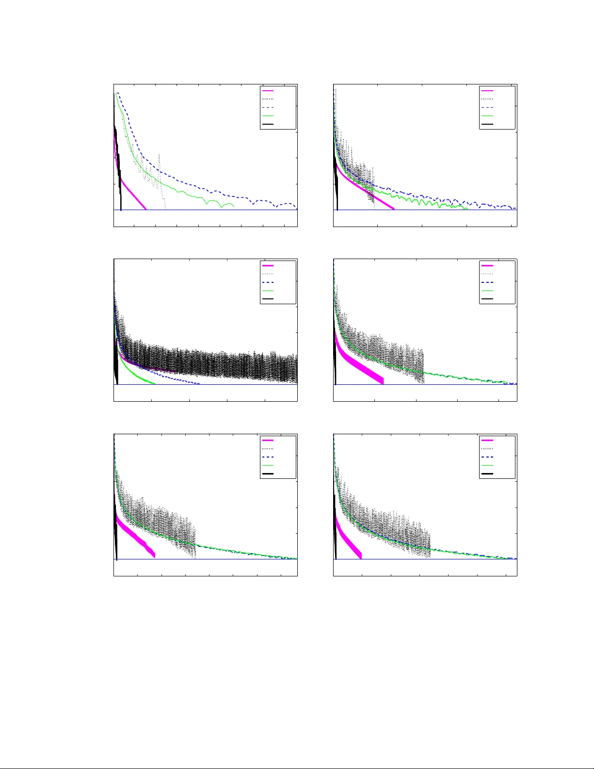
Sparse In v erse Co v ariance Estimation via an Adapti ve Gradient-Based Method Suvrit Sra ∗ Dongmin Kim Max Planck Institute for Intelligent Systems Uni versity of T exas at Austin T ¨ ubingen, Germany Austin, TX 78712 suvrit@tuebingen.mpg.de dmkim@cs.utexas.edu version of: June 3, 2010 Abstract W e study the problem of estimating from data, a sparse approximation to the in verse covariance matrix. Estimating a sparsity constrained in verse covariance matrix is a ke y component in Gaussian graphical model learning, but one that is numerically v ery challenging. W e address this challenge by de veloping a new adaptiv e gradient-based method that carefully combines gradient information with an adaptiv e step-scaling strategy , which results in a scalable, highly competitiv e method. Our algorithm, like its predecessors, maximizes an ` 1 -norm penalized log-likelihood and has the same per iteration arithmetic complexity as the best methods in its class. Our experiments re veal that our approach outperforms state-of-the-art competitors, often significantly so, for large problems. 1 Intr oduction A widely employed multi v ariate analytic tool is a Gaussian Markov Random Field (GMRF), which in essence, simply defines Gaussian distrib utions o ver an undirected graph. GMRFs are enormously useful; f amiliar applications include speech recognition [4], time-series analysis, semiparametric re gression, image analysis, spatial statistics, and graphical model learning [17, 29, 31]. In the context of graphical model learning, a key objecti ve is to learn the structure of a GMRF [29, 31]. Learning this structure often boils down to discovering conditional independencies between the variables, which in turn is equiv alent to locating zeros in the associated in verse co v ariance (precision) matrix Σ − 1 —because in a GMRF , an edge is present between nodes i and j , if and only if Σ − 1 ij 6 = 0 [17, 29]. Thus, estimating an in verse co v ariance matrix with zeros is a natural task, though formulating it in v olv es tw o obvious, b ut conflicting goals: (i) parsimony and (ii) fidelity . It is easy to ackno wledge that fidelity is a natural goal; in the GMRF setting it essentially means obtaining a statis- tically consistent estimate (e.g. under mild re gularity conditions a maximum-likelihood estimate [22]). But parsimony too is a valuable target. Indeed, it has long been recognized that sparse models are more robust and can even lead to better generalization performance [9]. Furthermore, sparsity has great practical value, because it: (i) reduces storage and subsequent computational costs (potentially critical to settings such as speech recognition [4]); (ii) leads to GM- RFs with fewer edges, which can speed up inference algorithms [20, 31]; (iii) rev eals interplay between variables and thereby aids structure discov ery , e.g., in gene analysis [10]. ∗ This w ork was done when SS was af filiated with the Max Planck Institute for Biological Cybernetics. W e finished this preprint on June 3, 2010, but ha ve uploaded it after more than a year to arXi v (in June 2011), so it is not the definiti ve v ersion of this work. 1 Achieving parsimonious estimates while simultaneously respecting fidelity is the central aim of the Sparse In- verse Cov ariance Estimation (SICE) problem. Recently , d’Aspremont et al. [8] formulated SICE by considering the penalized Gaussian log-likelihood [8] (omitting constants) log det( X ) − T r( S X ) − ρ X ij | x ij | , where S is the sample covariance matrix and ρ > 0 is a parameter that trades-of f between fidelity and sparsity . Maxi- mizing this penalized log-likelihood is a non-smooth concav e optimization task that can be numerically challenging for high-dimensional S (largely due to the positive-definiteness constraint on X ). W e address this challenge by dev elop- ing a new adaptiv e gradient-based method that carefully combines gradient information with an adaptive step-scaling strategy . And as we will later see, this care turns out to hav e a tremendous positive impact on empirical performance. Howe ver , before describing the technical details, we put our work in broader perspective by first enlisting the main contributions of this paper , and then summarizing related work. 1.1 Contributions This paper makes the follo wing main contrib utions: 1. It dev elops and ef ficient ne w gradient-based algorithm for SICE. 2. It presents associated theoretical analysis, formalizing key properties such as con ver gence. 3. It illustrates empirically not only our own algorithm, b ut also competing approaches. Our new algorithm has O ( n 3 ) arithmetic complexity per iteration like other competing approaches. Howe ver , our algorithm has an edge over many other approaches, because of three reasons: (i) the constant within the big-Oh is smaller , as we perform only one gradient ev aluation per iteration; (ii) the eigenv alue computation burden is reduced, as we need to only occasionally compute positiv e-definiteness; and (ii) the empirical con v ergence turns out to be rapid. W e substantiate the latter observ ation through e xperiments, and note that state-of-the-art methods, including the recent sophisticated methods of Lu [18, 19], or the simple but effecti v e method of [11], are both soundly outperformed by our method. Notation: W e denote by S n and S n + , the set of n × n symmetric, and semidefinite (  0 ) matrices, respecti vely . The matrix S ∈ S n + denotes the sample cov ariance matrix on n dimensional data points. W e use | X | to denote the matrix with entries | x ij | . Other symbols will be defined when used. 1.2 Related work, algorithmic appr oaches Dempster [9] was the first to formally in vestig ate SICE, and he proposed an approach wherein certain entries of the in v erse cov ariance matrix are explicitly set to zero, while the others are estimated from data. Another old approach is based on greedy forward-backward search, which is impractical as it requires O ( n 2 ) MLEs [17, 29]. More re- cently , Meinshausen and B ¨ uhlmann [21] presented a method that solves n different Lasso subproblems by regressing variables against each other: this approach is fast, b ut approximate, and it does not yield the maximum-likelihood estimator [8, 13]. An ` 1 -penalized log-likelihood maximization formulation of SICE was considered by [8] who introduced a nice block-coordinate descent scheme (with O ( n 4 ) per-iteration cost); their scheme formed the basis of the graphical lasso algorithm [13], which is much faster for very sparse graphs, but unfortunately has unkno wn theoretical complexity and its con ver gence is unclear [18, 19]. There exist numerous other approaches to SICE, e.g., the Cholesky-decomposition (of the inv erse cov ariance) based algorithm of [28], which is an expensi ve O ( n 4 ) per-iteration method. There are other Cholesky-based variants, but these are either heuristic [15], or limit attention to matrices with a known banded- structure [3]. Many generic approaches are also possible, e.g., interior-point methods [24] (usually too expensi ve for SICE), gradient-projection [2, 5, 11, 19, 27], or projected quasi-Newton [6, 30]. 2 Due to lack of space we cannot afford to giv e the various methods a surve y treatment, and restrict our attention to the recent algorithms of [18, 19] and of [11], as these seem to be over a broad range of inputs the most competiti ve methods. Lu [18] optimizes the dual (7) by applying Nesterov’ s techniques [23], obtaining an O (1 / √  ) iteration com- plexity algorithm (for  -accuracy solutions), that has O ( n 3 ) cost per iteration. He applies his framew ork to solve (1) (with R = ρee T ), though to improv e the empirical performance he deriv es a variant with slightly weaker theoretical guarantees. In [19], the author derives two “adapti v e” methods that proceed by solving a sequence of SICE problems with varying R . His first method is based on an adaptiv e spectral projected gradient [5], while second is an adap- tiv e version of his Nesterov style method from [18]. Duchi et al. [11] presented a simple, but surprisingly effecti ve gradient-projection algorithm that uses backtracking line-search initialized with a “good” guess for the step-size (ob- tained using second-order information). W e remark, howe ver , that ev en though Duchi et al.’ s algorithm [11] usually works well in practice, its con ver gence analysis has a subtle problem: the method ensures descent, but not sufficient descent, whereby the algorithm can “conv er ge” to a non-optimal point. Our express goal is the paper is to deriv e an algorithm that not only works better empirically , b ut is also guaranteed to con v erge to the true optimum. 1.3 Background: Problem f ormulation W e be gin by formally defining the SICE problem, essentially using a formulation deriv ed from [8, 11]: min X  0 F ( X ) = T r( S X ) − log det( X ) + T r( R | X | ) . (1) Here R ∈ S n is an elementwise non-negati v e matrix of penalty parameters; if its ij -entry r ij is large, it will shrink | x ij | tow ards zero, thereby gaining sparsity . Follo wing [19] we impose the restriction that S +Diag( R )  0 , where Diag( R ) is the diagonal (matrix) of R . This restriction ensures that (1) has a solution, and subsumes related assumptions made in [8, 11]. Moreover , by the strict con ve xity of the objecti ve, this solution is unique. Instead of directly solving (1), we also (like [8, 11, 18, 19]) focus on the dual as it is differentiable, and has merely bound constraints. A simple device to derive dual problems to ` 1 -constrained problems is [16]: introduce a new variable Z = X and a corresponding dual v ariable U . Then, the Lagrangian is L ( X, Z , U ) = T r( S Z ) − log det( Z ) + k R  X k 1 , 1 + T r( U ( Z − X )) . (2) The dual function g ( U ) = inf X,Z L ( X, Z , U ) . Computing this infimum is easy as it separates into infima ov er X and Z . W e ha ve inf Z T r( S Z ) − log det( Z ) + T r( U Z ) , (3) which yields S − Z − 1 + U = 0 , or Z = ( S + U ) − 1 . (4) Next consider inf X k R  X k 1 , 1 − T r( U X ) = inf X X ij ρ ij | x ij | − X ij u ij x ij , (5) which is unbounded unless | u ij | ≤ ρ ij , in which case it equals zero. This, with (4) yields the dual function g ( U ) = ( T r(( S + U ) Z ) − log det( Z ) | u ij | ≤ ρ ij , −∞ otherwise . (6) Hence, the dual optimization problem may be written as (dropping constants) min U − log det( S + U ) s.t. | u ij | ≤ ρ ij , i, j ∈ [ n ] . (7) 3 Observe that −∇G = ( S + U ) − 1 = X ; so we easily obtain the primal optimal solution from the dual-optimal. Defining, X U = ( S + U ) − 1 , the duality gap may be computed as F ( X U ) − G ( U ) = T r( S X U ) + T r( R | X U | ) − n. (8) Giv en this problem formalization we are no w ready to describe our algorithm. 2 Algorithm Broadly viewed, our new adaptive gradient-based algorithm consists of three main components: (i) gradient compu- tation; (ii) step-size computation; and (iii) “checkpointing” for positive-definiteness. Computation of the gradient is the main O ( n 3 ) cost that we (like other gradient-based methods), must pay at ev ery iteration. Even though we com- pute gradients only once per iteration, saving on gradient computation is not enough. W e also need a better strategy for selecting the step-size and for handling the all challenging positive-definiteness constraint. Unfortunately , both are easier said than done: a poor choice of step-size can lead to painfully slow con ver gence [2], while enforcing positiv e-definiteness requires potentially expensi ve eigen v alue computations. The key aspect of our method is a new step-size selection strategy , which helps greatly accelerate empirical conv er gence. W e reduce the unavoidable cost of eigen v alue computation by not performing it at ev ery iteration, b ut only at certain “checkpoint” iterations. Intuitiv ely , at a checkpoint the iterate must be tested for positive-definiteness, and failing satisfaction an alternate strategy (to be described) must be in voked. W e observed that in practice, most intermediate iterates generated by our method usually satisfy positiv e-definiteness, so the alternate strategy is triggered only rarely . Thus, the simple idea of checkpointing has a tremendous impact on performance, as borne through by our experimental results. Let us now formalize these ideas below . W e begin by describing our stepsize computation, which is deriv ed from the well-known Barzilai-Borwein (BB) stepsize [1] that was found to accelerate ( unconstrained ) steepest descent considerably [1, 7, 25]. Unfortunately the BB stepsizes do not work out-of-the-box for constrained problems, i.e., nai ¨ ıvely plugging them into gradient- projection does not work [7]. For constrained setups the spectral projected gradient (SPG) algorithm [5] is a popular method based on BB stepsizes combined with a globalization strategy such as non-monotone line-searches [14]. For SICE, very recently Lu [19] exploited SPG to de velop a sophisticated, adapti v e SPG algorithm for SICE. F or deri ving our BB-style stepsizes, we first recall that for unconstrained conve x quadratic problems, steepest-descent with BB is guaranteed to conv er ge [12]. This immediately suggests using an active-set idea, which says that if we could identify variables activ e at the solution, we could reduce the optimization to an unconstrained problem, which might be “easier” to solv e than its constrained counterpart. W e thus arri ve at our first main idea: use the active-set information to modify the computation of the BB step itself . This simple idea turns out to have a big impact on empirical consequences; we describe it below . W e partition the variables into active and working sets, and carry out the optimization over the working set alone. Moreov er , since gradient information is also a v ailable, we e xploit it to further refine the acti ve-set to obtain the binding set; both are formalized below . Definition 1. Giv en dual v ariable U , the active set A ( U ) and the binding set B ( U ) are defined as A ( U ) =  ( i, j )   | U ij | = ρ ij  , , (9) B ( U ) =  ( i, j )   U ij = − ρ ij , ∂ ij G ( U ) > 0 , or U ij = ρ ij , ∂ ij G ( U ) < 0  , (10) where ∂ ij G ( U ) denotes the ( i, j ) component of ∇G ( U ) . The role of the binding set is simple: variables bound at the current iteration are guaranteed to be active at the next. Specifically , let U =  U   | U ij | = ρ ij  , and denote orthogonal projection onto U by P U ( · ) , i.e., P U ( U ij ) = mid { U ij , − ρ ij , ρ ij } . (11) 4 If ( i, j ) ∈ B ( U k ) and we iterate U k +1 = P U  U k − γ k ∇G ( U k )  for some γ k > 0 , then since   U k +1 ij   =   P U  U k ij − γ k ∂ ij G ( U k )    = ρ ij , the membership ( i, j ) ∈ A ( U k +1 ) holds. Therefore, if we know that ( i, j ) ∈ B ( U k ) , we may discard U k ij from the update. W e now to employ this idea in conjunction with the BB step, and introduce our new modification: first compute B ( U k ) and then confine the computation of the BB step to the subspace defined by ( i, j ) / ∈ B ( U k ) . The last ingredient that we need is safe-guar d parameters σ min , σ max , which ensure that the BB-step computation is well- behav ed [14, 19, 26]. W e thus obtain our modified computation, which we call modified-BB (MBB) step: Definition 2 (Modified BB step) . ˜ σ = k ∆ ˜ U k − 1 k 2 F P i P j ∆ ˜ U k − 1 ij · ∆ ˜ G k − 1 ij · · · · · · ( a ) , or ˜ σ = P i P j ∆ ˜ U k − 1 ij · ∆ ˜ G k − 1 ij k ∆ ˜ G k − 1 k 2 F · · · · · · ( b ) , σ k = mid { σ min , ˜ σ , σ max } . (12) where ∆ ˜ U k − 1 and ∆ ˜ G k − 1 are defined by ov er only non-bound v ariables by the follo wing formulas: ∆ ˜ U k − 1 ij =  [ U k − 1 − U k − 2 ] ij , if ( i, j ) / ∈ B ( U k ) , 0 , otherwise . (13) ∆ ˜ G k − 1 ij =  [ ∇G k − 1 − ∇G k − 2 ] ij , if ( i, j ) / ∈ B ( U k ) , 0 , otherwise . (14) Assume for the moment that we did not have the positi ve-definite constraint. Even then, our MBB steps de- riv ed above, are not enough to ensure con v ergence. This is not surprising since even for the unconstrained gen- eral con v ex objecti v e case, ensuring con v ergence of BB-step-based methods, globalization (line-search) strategies are needed [14, 26]; the problem is only worse for constrained problems too, and some line-search is needed to ensure con v ergence [5, 12, 14]. The easy solution for us too would be in voke a non-monotone line-search strate gy . Howe v er , we observed that MBB step alone often produces conv er ging iterates, and even lazy line-search in the style of [7, 14] affects it adversely . Here we introduce our second main idea: T o retain empirical benefits of subspace steps while still guaranteeing conv er gence, we propose to scale the MBB stepsize using a diminishing scalar sequence, but not out-of-the-box; instead we propose to relax the application of diminishing scalars by introducing an “optimistic” di- minishment strate gy . Specifically , we scale the MBB step (12) with some constant scalar δ for a fixed number, say M , of iterations. Then, we check whether a descent condition is satisfied. If the current iterate passes the descent test, then the method continues for another M iterations with the same δ ; if it fails to satisfy the descent, then we diminish the scaling factor δ . This diminishment is “optimistic” because ev en when the method fails to satisfy the descent condition that triggered diminishment, we merely diminish δ once, and continue using it for the next M iterations. W e remark that superficially this strategy might seem similar to occasional line-search, but it is fundamentally different: unlike line-search our strategy does not enforce monotonicity after failing to descend for a prescribed number of iterations. W e formalize this belo w . Suppose that the method is at iteration c , and from there, iterates with a constant δ c for the next M iterations, so that from the current iterate U c , we compute U k +1 = P U  U k − δ c · σ k ∇G ( U k )  , (15) for k = c, c + 1 , · · · , c + M − 1 , where σ k is computed via (12)-(a) and (12)-(b) alternatingly . No w , at the iterate U c + M , we check the descent condition: 5 Definition 3 (Descent condition) . G ( U c ) − G ( U c + M ) ≥ κ X i X j ∂ ij G ( U c ) · [ U c − U c + M ] ij , (16) for some fixed parameter κ ∈ (0 , 1) . If iterate U c + M passes the test (16), then we reuse δ c and set δ c + M = δ c ; otherwise we diminish δ c and set δ c + M ← η · δ c , for some fixed η ∈ (0 , 1) . After adjusting δ c + M the method repeats the update (15) for another M iterations. Finally , we measure the duality gap ev ery M iterations to determine termination of the method. Explicitly , giv en a stopping threshold  > 0 , we define: Definition 4 (Stopping criterion) . F ( −∇G ( U )) − G ( U ) = F ( X U ) − G ( U ) = T r( S X U ) + T r( R | X U | ) − n < . (17) Algorithm 1 encapsulates all the abov e details, and presents pseudo-code of our algorithm SICE . Giv en U 0 and U 1 ; for i = 1 , · · · until the stopping criterion (17) met do ˜ U 0 ← U i − 1 and ˜ U 1 ← U i ; for j = 1 , · · · , M do /* Modified BB */ Compute B ( ˜ U j ) then compute σ j using (12)-(a) and -(b) alternatingly; ˜ U j +1 ← P U  ˜ U j − δ i · σ j ∇G ( ˜ U j )  ; if Is S + ˜ U  0 then if ˜ U M satisfies (16) then U i +1 ← ˜ U M , and δ i +1 ← δ i ; else /* Diminish Optimistically */ δ i +1 ← η δ i , where η ∈ (0 , 1) ; else Enforce posdef; ˜ U M ← ; if ˜ U M satisfies (16) then U i +1 ← ˜ U M , and δ i +1 ← δ i ; else /* Diminish Optimistically */ δ i +1 ← η δ i , where η ∈ (0 , 1) ; Algorithm 1: Sparse In v erse Cov ariance Estimation ( SICE ). 3 Analysis In this section we analyze theoretical properties of SICE . First, we establish con ver gence, and then briefly discuss some other properties. For clarity , we introduce some additional notation. Let M be the fixed number of modified-BB iterations, i.e., descent condition (16) is check ed only ev ery M iterations. W e index these M -th iterates with K = { 1 , M + 1 , 2 M + 1 , 3 M + 1 , · · · } , and then consider the sequence { U r } , r ∈ K generated by SICE . Let U ∗ denote the optimal solution to the problem. W e first show that such an optimal e xists. 6 Theorem 5 (Optimal) . If R > 0 , then there e xists an optimal U ∗ to (7) such that X ∗ ( S + U ∗ ) = I , and T r( X ∗ U ∗ ) = T r( R | X ∗ | ) . Pr oof. From [19, Proposition 2.2] (or the supplementary material), W e know that Problem (1) has a unique optimal solution X ∗ ∈ S n ++ . On the other hand, from [11, Lemma 1], there exists a feasible point U ∈ int ( U ) , thereby Slater’ s constraint qualification guarantees that the theorem holds. W e remind the reader that when proving conv ergence of iterativ e optimization routines, one often assumes Lips- chitz continuity of the objecti v e. W e, therefore be gin our discussion by stating the f act that the dual objecti v e function G ( U ) is indeed Lipschitz continuous. Proposition 6 (Lipschitz constant [18]) . The dual gradient ∇G ( U ) is Lipschitz continuous on U with Lipschitz con- stant L = λ 2 max ( X ∗ )(max ij r ij ) 2 . W e now prove that { U r } → U ∗ as r → ∞ . T o that end, suppose that the diminishment step δ c + M ← η · δ c is triggered only a finite number of times. Then, there exists a suf ficiently large K such that for all r ∈ K , r ≥ K , G ( U r ) − G ( U r +1 ) ≥ κ X i X j ∂ ij G ( U r ) · [ U r − U r +1 ] ij . In such as case, we may view the sequence { U r } as if it were generated by an ordinary gradient projection scheme, whereby the con ver gence { U r } → U ∗ follows using standard arguments [2]. Therefore, to prove the con ver gence of the entire algorithm, it suffices to discuss the case where the diminishment occurs infinitely often. Corresponding to an infinite sequence { U r } , there is a sequence { δ r } , which by construction is diminishing. Hence, if we impose the following unbounded sum condition on this sequence, follo wing [2], we can again ensure con ver gence. Definition 7 (Diminishing with unbounded sum) . (i) lim r →∞ δ r = 0 , and (ii) lim r →∞ X r i =1 δ i = ∞ . Since in our algorithm, we scale the MBB step (12) σ r by a diminishing scalar δ r , we must ensure that the resulting sequence δ r α r also satisfies the abov e condition. This is easy , but for the reader’ s con venience formalized belo w . Proposition 8. In Algorithm 1, the stepsize δ r · σ r satisfies the condition 7. Pr oof. Since lim r →∞ δ r = 0 and lim r →∞ P r i =1 δ i = ∞ by construction, lim r →∞ δ r · σ r ≤ σ max · lim r →∞ δ r = 0 and lim r →∞ r X i =1 δ i · σ i ≥ σ min · lim r →∞ r X i =1 δ i = ∞ . Using this proposition we can finally state the main conv er gence theorem. Our proof is based on that of gradient- descent; we adapt it for our problem by showing some additional properties of { U r } . Theorem 9 (Con ver gence) . The sequence of iterates ( X k , U k ) generated by Algorithm 1 conver ges to the optimum solution ( X ∗ , U ∗ ) . Pr oof. Consider the update (15) of Algorithm 1, we can rewrite it as U r +1 = U r + δ r · σ r D r , (18) 7 where the descent dir ection D r satisfies D r ij =    0 , if ( i, j ) ∈ B ( U r ) , − mid  U r ij − ρ ij δ r · σ r , U r ij + ρ ij δ r · σ r , ∂ ij G ( U r )  , otherwise . (19) Using (19) and the fact that there e xists at least one | ∂ ij G ( U r ) | > 0 unless U r = U ∗ , we can conclude that there exists a constant c 1 > 0 such that − X i X j ∂ ij G ( U r ) · D r ij ≥ X ( i,j ) / ∈B ( U r ) m 2 ij ≥ c 1 k∇G ( U r ) k 2 F > 0 , (20) where m ij = mid n U r ij − ρ ij δ r · σ r , U r ij + ρ ij δ r · σ r , ∂ ij G ( U r ) o . Similarly , we can also show that there e xists c 2 > 0 such that k D r k 2 F ≤ c 2 k∇G ( U r ) k 2 F . (21) Finally , using the inequalities (20) and (21), in conjunction with Proposition 6, 8, the proof is immediate from Propo- sition 1.2.4 in [2]. 4 Numerical Results W e present numerical results on both synthetic as well as real-world data. W e begin with the synthetic setup, which helps to position our method via--vis the other competing approaches. W e compare against algorithms that represent the state-of-the-art in solving the SICE problem. Specifically , we compare the following 5 methods: (i) PG : the pro- jected gradient algorithm of [11]; 1 (ii) ASPG : the very recent adaptiv e spectral projected gradient algorithm [19]; 2 (iii) ANES : an adaptiv e, Nesterov style algorithm from the ASPG paper [19]; 2 (iv) SCO V : a sophisticated smooth optimization scheme built on Nestero v’ s techniques [18]; 3 and (v) SICE : our proposed algorithm. W e note at this point that although due to space limits our experimentation is not exhausti ve, it is fairly extensi ve. Indeed, we also tried several other baseline methods such as: gradient projection with Armijo-search rule [2], limited memory projected quasi-Newton approaches [6, 30], among others. But all these approaches performed across wide range of problems similar to or worse than PG . Hence, we do not report numerical results against them. W e further note that Lu [18] reports the SCOV method vastly outperforms block-coordinate descent (BCD) based approaches such as [8], or ev en the graphical lasso FOR TRAN code of Friedman et al. [13]. Hence, we also omit BCD methods from our comparisons. 4.1 Synthetic Data Experiments W e generated random instances in the same manner as d’Aspremont et al. [8]; the same data generation scheme was also used by Lu [18, 19], and to be fair to them, we in fact used their M A T L A B code to generate our data (this code is included in the supplementary material for the interested reader). First one samples a sparse, inv ertible matrix S 0 ∈ S n , with ones on the diagonal, and having a desired density δ obtained by randomly adding +1 and − 1 off- diagonal entries. Then one perturbs S 0 to obtain S 00 = ( S 0 ) − 1 + τ N , where N ∈ S n is an i.i.d. uniformly random matrix. Finally , one obtains S , the random sample covariance matrix by shifting the spectrum of S 00 by S = S 00 − min { λ min ( S 00 ) − ς , 0 } I , where ς > 0 is a small scalar . The specific parameter v alues used were the same as in [18], namely: δ = . 01 , τ = . 15 , and ς = 10 − 4 . W e generated matrices of size 100 m × 100 m , for m ∈ [1 . . . 10] ∪ { 16 , 20 } . 1 Impl. 2 Downloaded from 3 Downloaded from 8  PG ASPG ANES SCO V SICE 1E-01 8.46 38.97 48.05 21.75 2.28 1E-02 34.89 72.25 100.61 46.10 4.74 1E-03 127.37 142.47 214.56 98.73 7.61 1E-04 807.16 519.37 482.97 224.58 17.30 2E-05 - 1914.33 862.86 409.06 42.38 1E-05 - 2435.14 1149.04 548.34 52.29  PG ASPG ANES SCO V SICE 1E-01 128.61 1005.98 1818.00 1858.70 66.08 1E-02 358.90 1712.01 3173.55 3216.55 102.48 1E-03 833.86 3529.29 5411.49 5085.51 170.25 1E-04 1405.56 5008.81 9528.91 9046.04 234.18 2E-05 - 6420.18 15964.26 15428.23 307.67 1E-05 - 7562.52 19812.06 19621.27 336.25 T able 1: Time (secs) for reaching desired duality gap. Left, S ∈ S 300 + , and right, S ∈ S 1000 + . Since all algorithms decrease the duality-gap non-monotonically , we show the time-points when a prescribed  is first attained. T able 1 shows two sample results (more extensiv e results are available in the supplementary material). All the algorithms were run with a con v ergence tolerance of  = 2 · 10 − 5 ; this tolerance is very tight, as previously reported results usually used  = . 1 or . 01 . T able 1 reveals two main results: (i) the advanced algorithms of [18, 19] are out- performed by both PG and SICE ; and (ii) SICE vastly outperforms all other methods. The first result can be attributed to the algorithmic simplicity of PG and SICE , because ASPG , ANES , and SCO V employ a complex, more expensi ve algorithmic structure: the y repeatedly use eigendecompositions. The second result, that is, the huge difference in performance between PG and SICE (see T able 1, second sub-table, fourth and fifth rows) is also easily explained. Al- though the step-size heuristic used by PG works very-well for obtaining low accuracy solutions, for slightly stringent con v ergence criteria its progress becomes much too slow . SICE on the other hand, exploits the gradient information to rapidly identify the active-set, and thereby exhibits faster conv er gence. In fact, SICE turns out to be even faster for low accurac y (  = . 1 ) solutions. The con ver gence behavior of the various methods is illustrated in more detail in Figure 1. The left panel plots the duality gap attained as a function of time, which makes the performance differences between the methods starker: SICE con v erges rapidly to a tight tolerance in a fraction of the time needed by other methods. The right panel summarizes performance profiles as the input matrix size n × n is varied. Even as a function of n , SICE is seen to be ov erall much faster (y-axis is on a log scale) than other methods. 50 100 150 200 10 −5 10 −3 10 −1 10 1 10 3 Running time (seconds) Duality gap ε PG ASPG ANES SCOV SICE 2000 4000 6000 8000 10000 12000 10 −5 10 −3 10 −1 10 1 10 3 Running time (seconds) Duality gap ε PG ASPG ANES SCOV SICE 200 400 600 800 1000 10 0 10 1 10 2 10 3 Size of matrix (n x n) Running time (seconds) Duality gap: ε =1.0E−02 PG ASPG ANES SCOV SICE 200 400 600 800 1000 10 0 10 1 10 2 10 3 Size of matrix (n x n) Running time (seconds) Duality gap: ε =1.0E−04 PG ASPG ANES SCOV SICE Figure 1: Left panel: duality g ap attained as a function of running time (in seconds); Right panel: Time taken to reach a prescribed duality gap as a function of matrix S ’ s size. 5 Conclusions and futur e work W e dev eloped, analyzed, and experimented with a powerful new algorithm for estimating the sparse in verse cov ariance matrices. Our method was shown to outperform all the competing state-of-the-art approaches. W e attribute the speedup gains to our careful algorithmic design, which also shows that even though the spectral projected gradient method is fast and often successful, in v oking it out-of-the-box can be a suboptimal approach in scenarios where the constraints were simple. In such as setup, our modified spectral approach turns out to afford significant empirical gains. 9 At this point sev eral avenues of future work are open. W e list them in order of difficulty: (i) Implementing our method in a multi-core or GPU setting; (ii) Extending our approach to handle more general constraints; (iii) Deriving an e v en more ef ficient algorithm that only occasionally computes gradients; (i v) Deri ving a method for SICE that does not need to explicitly compute matrix in verses. Refer ences [1] J. Barzilai and J. M. Borwein. T wo-Point Step Size Gradient Methods. IMA Journal of Numerical Analysis , 8(1):141–148, 1988. [2] D. P . Bertsekas. Nonlinear Pr ogr amming . Athena Scientific, second edition, 1999. [3] P . J. Bickel and E. Le vina. Regularized estimation of large cov ariance matrices. Ann. Statist. , 36(1):199–227, 2008. [4] J. A. Bilmes. Factored sparse in verse co variance matrices. In IEEE ICASSP , 2000. [5] E. G. Birgin, J. M. Mart ´ ınez, and M. Raydan. Nonmonotone Spectral Projected Gradient Methods on Conv ex Sets. SIAM Journal on Optimization , 10(4):1196–1211, 2000. [6] R. Byrd, P . Lu, J. Nocedal, and C. Zhu. A Limited Memory Algorithm for Bound Constrained Optimization. SIAM J . Sci. Comp. , 16(5):1190–1208, 1995. [7] Y . H. Dai and R. Fletcher . Projected Barzilai-Borwein Methods for Large-scale Box-constrained Quadratic Programming. Numerische Mathematik , 100(1):21–47, 2005. [8] A. d’Aspremont, O. Banerjee, and L. E. Ghaoui. First-order methods for sparse co v ariance selection. SIAM J . Matrix Anal. Appl. , 30(1):56–66, 2008. [9] A. P . Dempster . Cov ariance selection. Biometrics , 28(1):157–175, 1972. [10] A. Dobra, C. Hans, B. Jones, J. R. Ne vins, and M. W est. Sparse graphical models for exploring gene e xpression data. J ournal of Multivariate Analysis , 90:196–212, 2004. [11] J. Duchi, S. Gould, and D. K oller . Projected subgradient methods for learning sparse Gaussians. In Pr oc. Uncertainty in Artificial Intelligence , 2008. [12] A. Friedlander , J. M. Mart ´ ınez, and M. Raydan. A New Method for Large-scale Box Constrained Conv ex Quadratic Mini- mization Problems. Optimization Methods and Software , 5:55–74, 1995. [13] J. Friedman, T . Hastie, and R. T ibshirani. Sparse inv erse covariance estimation with the graphical lasso. Biostatistics , 9: 432–441, 2008. [14] L. Grippo and M. Sciandrone. Nonmonotone Globalization T echniques for the Barzilai-Borwein Gradient Method. Compu- tational Optimization and Applications , 23:143–169, 2002. [15] J. Z. Huang, N. Liu, M. Pourahmadi, and L. Liu. Covariance matrix selection and estimation via penalised normal likelihood. Biometrika , 93(1):85–98, 2006. [16] S. Kim, K. Koh, M. Lustig, S. Boyd, and D. Gorinevsky. An Interior-Point Method for Large-Scale ` 1 -Regularized Least Squares. IEEE J. Selected T opics in Signal Pr ocessing , 1:606–617, Dec. 2007. [17] S. L. Lauritzen. Graphical Models . OUP , 1996. [18] Z. Lu. Smooth optimization approach for sparse cov ariance selection. SIAM J. Optim. (SIOPT) , 19(4):1807–1827, 2009. [19] Z. Lu. Adapti v e first-order methods for general sparse in verse cov ariance selection. SIAM J. Matrix Analysis and Applications (SIMAX) , 31(4):2000–2016, 2010. [20] D. M. Malioutov , J. K. Johnson, and A. S. W illsky . W alk-Sums and Belief Propagation in Gaussian Graphical Models. JMLR , 7:2031–2064, 2006. [21] N. Meinshausen and P . B ¨ uhlmann. High-dimensional graphs and v ariable selection with the lasso. The Annals of Statistics , 34(3):1436–1462, 2006. [22] A. M. Mood, F . A. Graybill, and D. C. Boes. Introduction to the theory of statistics . McGraw-Hill, 1974. [23] Y . Nesterov . Smooth minimization of non-smooth functions. Math. Pro gram., Ser . A , 103:127–152, 2005. [24] Y . E. Nesterov and A. S. Nemirovski. Interior-P oint P olynomial Algorithms in Con vex Pro gramming: Theory and Applica- tions . SIAM, 1994. [25] M. Raydan. On the Barzilai and Borwein Choice of the Steplength for the Gradient Method. IMA Journal on Numerical Analysis , 13:321–326, 1993. [26] M. Raydan. The Barzilai and Borwein gradient method for the large scale unconstrained minimization problem. SIAM J. Opt. , 7(1):26–33, 1997. 10 [27] J. B. Rosen. The Gradient Projection Method for Nonlinear Programming. Part I. Linear Constraints. Journal of the Society for Industrial and Applied Mathematics , 8(1):181–217, 1960. [28] A. J. Rothman, P . J. Bickel, E. Levina, and J. Zhu. Sparse permutation inv ariant covariance estimation. Electr on. J. Statist. , 2:494–515, 2008. [29] H. Rue and L. Held. Gaussian Markov Random F ields . Chapman and Hall/CRC, 2005. [30] M. Schmidt, E. van den Berg, M. Friedlander, and K. Murphy . Optimizing Costly Functions with Simple Constraints: A Limited-Memory Projected Quasi-Newton Algorithm. In AIST A TS , 2009. [31] M. J. W ainwright and M. I. Jordan. Graphical Models, Exponential Families , and V ariational Inference. F ound. T rends Mach. Learn. , 1(1-2):1–305, 2008. A Additional numerical r esults  PG ASPG ANES SCO V SICE 1E-01 0.09 0.51 0.74 0.51 0.12 1E-02 0.14 0.62 1.10 0.75 0.14 1E-03 0.26 0.94 1.73 1.16 0.16 1E-04 0.52 1.17 2.87 1.93 0.20 2E-05 0.70 1.23 3.77 2.52 0.20 1E-05 0.78 1.26 4.31 2.86 0.20  PG ASPG ANES SCOV SICE 1E-01 1.70 6.40 8.48 6.04 0.94 1E-02 7.15 13.23 18.33 13.21 1.82 1E-03 22.79 27.00 43.98 31.79 2.97 1E-04 45.38 38.91 90.84 65.76 4.44 2E-05 61.46 46.53 162.22 118.36 4.80 1E-05 68.50 46.69 206.81 151.32 4.81 100 × 100 200 × 200  PG ASPG ANES SCO V SICE 1E-01 8.46 38.97 48.05 21.75 2.28 1E-02 34.89 72.25 100.61 46.10 4.74 1E-03 127.37 142.47 214.56 98.73 7.61 1E-04 807.16 519.37 482.97 224.58 17.30 2E-05 - 1914.33 862.86 409.06 42.38 1E-05 - 2435.14 1149.04 548.34 52.29  PG ASPG ANES SCO V SICE 1E-01 16.27 84.71 109.95 109.04 5.42 1E-02 51.89 150.26 226.52 226.34 9.46 1E-03 139.73 338.29 471.29 473.33 15.59 1E-04 357.93 769.44 1020.82 1027.13 25.84 2E-05 529.69 997.44 1776.06 1793.75 28.43 1E-05 603.84 1099.55 2221.23 2106.44 30.52 300 × 300 400 × 400  PG ASPG ANES SCO V SICE 1E-01 25.28 153.41 209.90 218.42 9.55 1E-02 66.44 262.69 428.14 437.31 16.42 1E-03 307.73 731.48 901.46 911.02 29.82 1E-04 631.33 1318.33 1788.93 1828.57 45.81 2E-05 815.42 1615.56 3069.17 3117.44 61.81 1E-05 - 1719.70 3821.50 3853.45 66.20  PG ASPG ANES SCO V SICE 1E-01 28.36 275.36 391.94 379.74 16.02 1E-02 87.15 499.69 744.94 728.40 27.69 1E-03 244.11 1082.84 1446.27 1365.46 49.70 1E-04 570.52 2088.16 2777.44 2660.26 75.53 2E-05 848.27 2952.95 5049.04 4873.74 88.16 1E-05 972.13 3379.78 6383.01 6130.96 99.84 500 × 500 600 × 600  PG ASPG ANES SCO V SICE 1E-01 96.06 291.24 422.53 327.12 28.36 1E-02 271.98 520.65 796.86 618.35 54.58 1E-03 496.38 925.59 1480.13 1155.40 80.02 1E-04 863.83 1332.72 2878.07 2251.48 118.62 2E-05 1133.74 2042.25 4776.05 3736.78 134.46 1E-05 1162.10 2077.83 6106.81 4614.11 141.79  PG ASPG ANES SCO V SICE 1E-01 110.74 609.90 956.90 942.62 30.17 1E-02 320.52 880.04 1742.28 1720.76 46.54 1E-03 785.29 1742.65 3106.48 3099.92 73.06 1E-04 1742.95 3287.96 5931.33 5925.93 124.42 2E-05 2523.65 4557.51 10083.89 10018.28 175.97 1E-05 - 5470.64 12656.09 12494.52 199.07 700 × 700 800 × 800  PG ASPG ANES SCO V SICE 1E-01 88.40 635.09 1306.82 1217.88 32.21 1E-02 245.25 1153.18 2331.24 2158.39 63.42 1E-03 816.69 2862.34 4053.39 3869.56 108.35 1E-04 1604.22 5424.09 7216.28 7538.87 184.97 2E-05 2117.68 6974.25 11973.47 12710.25 211.80 1E-05 2117.68 7907.47 15083.79 15784.19 242.39  PG ASPG ANES SCO V SICE 1E-01 128.61 1005.98 1818.00 1858.70 66.08 1E-02 358.90 1712.01 3173.55 3216.55 102.48 1E-03 833.86 3529.29 5411.49 5085.51 170.25 1E-04 1405.56 5008.81 9528.91 9046.04 234.18 2E-05 - 6420.18 15964.26 15428.23 307.67 1E-05 - 7562.52 19812.06 19621.27 336.25 900 × 900 1000 × 1000 11 0.5 1 1.5 2 2.5 3 3.5 4 10 −5 10 −3 10 −1 10 1 10 3 Running time (seconds) Duality gap ε PG ASPG ANES SCOV SICE 50 100 150 200 10 −5 10 −3 10 −1 10 1 10 3 Running time (seconds) Duality gap ε PG ASPG ANES SCOV SICE n = 100 n = 200 500 1000 1500 2000 10 −5 10 −3 10 −1 10 1 10 3 Running time (seconds) Duality gap ε PG ASPG ANES SCOV SICE 500 1000 1500 2000 10 −5 10 −3 10 −1 10 1 10 3 Running time (seconds) Duality gap ε PG ASPG ANES SCOV SICE n = 300 n = 400 500 1000 1500 2000 2500 3000 3500 10 −5 10 −3 10 −1 10 1 10 3 Running time (seconds) Duality gap ε PG ASPG ANES SCOV SICE 1000 2000 3000 4000 5000 6000 10 −5 10 −3 10 −1 10 1 10 3 Running time (seconds) Duality gap ε PG ASPG ANES SCOV SICE n = 500 n = 600 12 1000 2000 3000 4000 5000 6000 10 −5 10 −3 10 −1 10 1 10 3 Running time (seconds) Duality gap ε PG ASPG ANES SCOV SICE 2000 4000 6000 8000 10000 12000 10 −5 10 −3 10 −1 10 1 10 3 Running time (seconds) Duality gap ε PG ASPG ANES SCOV SICE n = 700 n = 800 2000 4000 6000 8000 10000 12000 14000 10 −5 10 −3 10 −1 10 1 10 3 Running time (seconds) Duality gap ε PG ASPG ANES SCOV SICE 5000 10000 15000 10 −5 10 −3 10 −1 10 1 10 3 Running time (seconds) Duality gap ε PG ASPG ANES SCOV SICE n = 900 n = 1000 13