Relative Density-Ratio Estimation for Robust Distribution Comparison

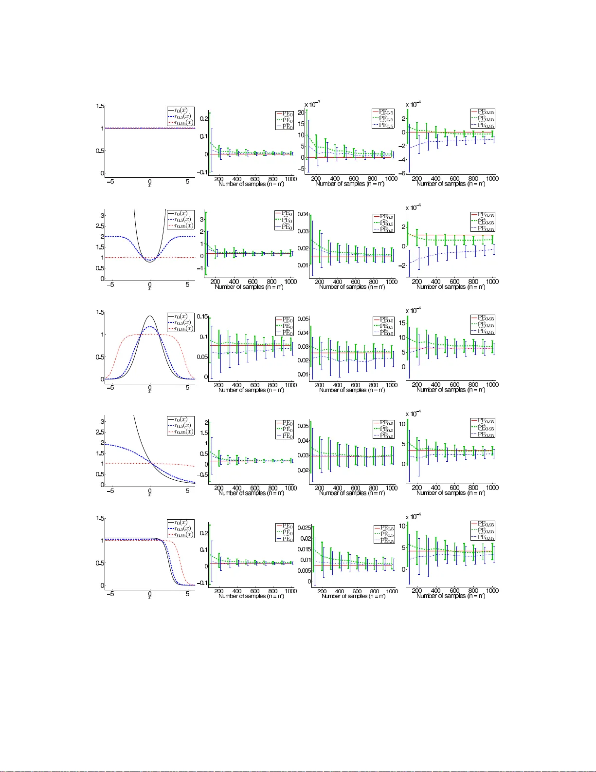
Relativ e Densit y-Ratio Estimati on for Ro bust Distribution Comparison Mak oto Y amada y amada@sg.cs.titech.a c.jp T okyo Institute of T e chnolo gy 2-12-1 O-okayama, Me gur o-ku, T okyo 1 52-8552 , Jap an. T aiji Suzuki s-t aiji@st a t. t.u-tokyo.ac.jp The University of T okyo 7-3-1 Hongo, Bun kyo-ku, T okyo 113-865 6, Jap an. T ak afumi Kanamori kanamori@is.nago y a-u.ac.jp Nagoya University F ur o cho, Chikusaku, Nagoya 464-8603, Jap an. Hirotak a Hachiy a hachiy a@sg.cs. titech.ac.jp T okyo Institute of T e chnolo gy 2-12-1 O-okayama, Me gur o-ku, T okyo 152-8552 , Jap an. Masashi Sugiy ama sugi@cs.titech.ac.jp T okyo Institute of T e chnolo gy 2-12-1 O-okayama, Me gur o-ku, T okyo 152-8552 , Jap an. Editor: ??? Abstract Div ergence e s timators based on direct approximation o f density-ratios without go ing through separate approximation of numerator and denomina to r densities hav e b een success- fully applied to m achine learning ta s ks that inv olve distribution compariso n s uch a s outlier detection, transfer learning, and t wo-sample homoge neit y test. How ever, since density-ratio functions often poss ess high ﬂuctuation, divergence es timation is still a challenging task in practice. In this pap er, we pr op ose to use r elative diver genc es for distribution compa ri- son, which involv es appr oximation of r elativ e density-ra tios . Since r elative density-ratios are alwa ys smo other than cor resp onding or dinary densit y-ratios , our pro p osed metho d is fav o rable in terms of the non-pa rametric conv ergence sp eed. F urthermore, we show that the prop osed divergence estimator has asymptotic v ariance indep endent o f the mo del com- plexity under a parametric setup, implying tha t the prop osed estimator hardly ov erﬁts even with complex mo dels. Through exp eriments, we demo ns trate the usefulness of the prop osed approach. Keyw ords: Densit y ratio, Pearson divergence, Outlier detection, Two-sample homogene- it y test, Unconstrained least-s q uares importance ﬁtting. 1. In t ro duction Comparing probabilit y distrib u tions is a fu ndamenta l task in statistical data pr o cessing. It can b e used for, e.g., outlier dete ction (Smola et al., 2009; Hido et al., 2011), two- sample homo geneity test (Gretton et al., 2007; Su giy ama et al., 2011), and tr ansfer le arning (Shimo daira, 2000 ; Su giy ama et al., 2007). Y amad a, Suz uki, Kana mori, H achiy a, and Sugiy ama A standard approac h to comparing probabilit y densities p ( x ) and p ′ ( x ) would b e to estimate a div ergence from p ( x ) to p ′ ( x ), suc h as the Kul lb ack-L eibler (KL) diver genc e (Kullbac k and Leibler, 1951): KL[ p ( x ) , p ′ ( x )] := Z log  p ( x ) p ′ ( x )  p ( x )d x . A naiv e w a y to estimate the KL divergence is to separately approxima te the densities p ( x ) and p ′ ( x ) from data and p lu g the estimated densities in the ab ov e d eﬁnition. Ho wev er, since densit y estimatio n is kno wn to b e a hard task (V apnik, 1998), this approac h do es not w ork we ll u nless a go o d parametric mo del is a v ailable. Recent ly , a d iv ergence estimation approac h wh ic h directly appro ximates the density r atio , r ( x ) := p ( x ) p ′ ( x ) , without going through separate appro ximation of densities p ( x ) an d p ′ ( x ) has b een pr op osed (Sugiy ama et al., 2008; Nguyen et al., 2010). Suc h d ensit y-ratio app ro ximation m etho ds w ere pr o v ed to ac hiev e the optimal non-parametric con v er gence rate in the m ini-max s ense. Ho wev er, the K L div ergence estimation via density-ratio app ro ximation is computation- ally rather exp ens ive du e to the non-linearit y in tro duced by the ‘log’ term. T o cop e with this problem, anot her div ergence called the Pe arson (PE) diver genc e (P earson, 1900) is useful. The PE div ergence f rom p ( x ) to p ′ ( x ) is deﬁn ed as PE[ p ( x ) , p ′ ( x )] := 1 2 Z  p ( x ) p ′ ( x ) − 1  2 p ′ ( x )d x . The PE div ergence is a squared-loss v arian t of the KL div ergence, and they b oth b elong to the class of the A li-Silvey-Csisz´ ar diver genc es (whic h is al so kno wn as the f -diver genc es , see Ali and Silv ey, 1966; Csisz´ ar, 1967 ). Th us, the PE and K L d iv ergences share similar prop erties, e.g., they are non -n egativ e and v anish if and only if p ( x ) = p ′ ( x ). Similarly to the KL divergence estimation, the PE div ergence can also b e accurately estimated based on densit y-ratio appro ximation (Kan amori et al., 2009): the den sit y- ratio approximat or called unc onstr aine d le ast-squar es imp ortanc e ﬁtting (uLSIF) giv es the PE div ergence estimator analyt ic al ly , wh ic h can b e computed ju s t b y solving a system of linear equations. The practical usefulness of the uLSIF-based PE div ergence esti- mator wa s d emons trated in v arious app lications such as outlier d etectio n (Hido et al., 2011), t w o-sa mple h omogeneit y test (Sugiy ama et al., 2011), and dimensionalit y reduction (Suzuki and Su giy ama, 2010). In this paper, we ﬁrs t establish the non-parametric conv ergence rate of the u L SIF-based PE div ergence estimator, w hic h elucidates its sup erior theoretical pr op erties. How eve r, it also rev eals that its con v ergence r ate is actually go v erned by the ‘sup ’-norm of the tru e densit y-ratio function: max x r ( x ). T his imp lies that, in the region where the denominator densit y p ′ ( x ) tak es s mall v alues, the d en sit y r atio r ( x ) = p ( x ) /p ′ ( x ) tends to take large v alues and therefore the o v erall conv ergence sp eed b ecomes slo w. More critically , den s it y ratios can ev en dive rge to inﬁnity u nder a rather simple setting, e.g. , w h en the ratio of t w o G aussian f u nctions is considered (Cortes et al., 2010). Th is makes the p aradigm of div ergence estimation based on dens ity-ratio approxima tion u nreliable. 2 Rela tive Density-Ra tio Estima tion In order to o v ercome this fund amen tal problem, we prop ose an alternativ e approac h to distribution comparison called α -r elative diver genc e e stimation . In the prop osed approac h, w e estimate the quantit y called th e α - r elative diver ge nc e , whic h is the div ergence from p ( x ) to th e α -mixtur e density αp ( x ) + (1 − α ) p ′ ( x ) for 0 ≤ α < 1. F or examp le, the α -relativ e PE divergence is given by PE α [ p ( x ) , p ′ ( x )] := PE[ p ( x ) , αp ( x ) + (1 − α ) p ′ ( x )] = 1 2 Z  p ( x ) αp ( x ) + (1 − α ) p ′ ( x ) − 1  2  αp ( x ) + (1 − α ) p ′ ( x )  d x . W e estimate the α -relativ e div ergence by d irect app ro ximation of the α -r elative d ensity- r atio : r α ( x ) := p ( x ) αp ( x ) + (1 − α ) p ′ ( x ) . A notable adv ant age of this approac h is that th e α -relativ e densit y-ratio is alw a ys b ound ed ab o v e by 1 /α when α > 0, ev en when th e ordin ary d ensit y-ratio is u nb ound ed . Based o n this feature, we theoretically show that the α -r elativ e PE div ergence estima- tor based on α -relativ e densit y-ratio app ro ximation is more fa v orable than the ordinary densit y-ratio app roac h in terms of the non-parametric conv ergence s p eed. W e further prov e that, under a co rrectly-sp eciﬁed parametric setup, the asymp totic v ariance of our α -relativ e PE d iv ergence estimator do es not dep end on the mo del complexit y . This means t hat the prop osed α -rela tiv e PE div ergence estimator hardly ov erﬁts ev en with complex mo dels. Through extensive exp eriments on outlier d etection, tw o-sample homogeneit y test, and transfer learning, we demonstrate that our pr op osed α -relativ e PE diverge nce estimator compares f av orably with alternativ e app roac h es. The rest of this pap er is structured as follo w s. In Sect ion 2, our prop osed relativ e PE d iv ergence estimator is d escrib ed. In S ection 3, w e provide n on-parametric analysis of the conv ergence rate and parametric analysis of the v ariance of the p r op osed PE div er- gence estimator. In Section 4, we exp erimen tally ev aluate the p erformance of th e prop osed metho d on v arious tasks. Finally , in Section 5, w e conclude the p ap er by summarizing our con tributions and describin g futur e p rosp ects. 2. Estimation of Relative P earson Divergence via Least-Squares Relativ e Densit y-Ratio Appro ximation In this section, we p r op ose an estimator of th e relativ e P earson (PE) diverge nce based on least-squares relativ e d ensit y-ratio appr o ximatio n. 2.1 Problem F orm ulation Supp ose we are giv en ind ep endent and identica lly d istributed (i.i.d.) samp les { x i } n i =1 from a d -dimensional d istribution P with densit y p ( x ) and i.i.d. samples { x ′ j } n ′ j =1 from another 3 Y amad a, Suz uki, Kana mori, H achiy a, and Sugiy ama d -dimensional d istribution P ′ with den sit y p ′ ( x ): { x i } n i =1 i . i . d . ∼ P , { x ′ j } n ′ j =1 i . i . d . ∼ P ′ . The goal of this pap er is to compare the tw o un derlying distribu tions P and P ′ only usin g the tw o sets of samp les { x i } n i =1 and { x ′ j } n ′ j =1 . F or 0 ≤ α < 1, let q α ( x ) b e the α -mixtur e density of p ( x ) and p ′ ( x ): q α ( x ) := αp ( x ) + (1 − α ) p ′ ( x ) . Let r α ( x ) b e the α -r elative density-r atio of p ( x ) and p ′ ( x ): r α ( x ) := p ( x ) αp ( x ) + (1 − α ) p ′ ( x ) = p ( x ) q α ( x ) . (1) W e deﬁne the α -r elative PE diver genc e from p ( x ) to p ′ ( x ) as PE α := 1 2 E q α ( x )  ( r α ( x ) − 1) 2  , (2) where E p ( x ) [ f ( x )] denotes the exp ectatio n of f ( x ) und er p ( x ): E p ( x ) [ f ( x )] = Z f ( x ) p ( x )d x . When α = 0, PE α is reduced to the ordinary PE dive rgence. T h us, t he α -relativ e PE div ergence can b e r egarded as a ‘sm o othed’ extension of the ordinary PE d iv ergence. Belo w, w e giv e a metho d for estimating the α - relativ e PE div ergence based on the appro ximation of the α -relativ e d ensit y-ratio. 2.2 Direct Appro ximation of α -Relativ e Densit y-Ratios Here, we describ e a metho d for appr o ximating the α -relativ e density-rat io (1). Let u s mo del the α -relativ e density-rati o r α ( x ) by the follo wing k ernel mo d el: g ( x ; θ ) := n X ℓ =1 θ ℓ K ( x , x ℓ ) , where θ := ( θ 1 , . . . , θ n ) ⊤ are parameters to b e learned fr om d ata samples, ⊤ denotes the transp ose of a matrix or a v ector, and K ( x , x ′ ) is a kernel basis fu nction. In the exp erimen ts, w e use the Gaussian k ernel: K ( x , x ′ ) = exp  − k x − x ′ k 2 2 σ 2  , where σ ( > 0) is th e kernel width. 4 Rela tive Density-Ra tio Estima tion The parameters θ in th e mo del g ( x ; θ ) are determined so that the follo win g exp ected squared-error J is minimized: J ( θ ) := 1 2 E q α ( x ) h ( g ( x ; θ ) − r α ( x )) 2 i = α 2 E p ( x )  g ( x ; θ ) 2  + (1 − α ) 2 E p ′ ( x )  g ( x ; θ ) 2  − E p ( x ) [ g ( x ; θ )] + C onst ., where we used r α ( x ) q α ( x ) = p ( x ) in the third term. Appr o ximating the exp ectat ions by empirical av erages, we obtain th e follo wing optimizatio n p roblem: b θ := argmin θ ∈ R n  1 2 θ ⊤ c H θ − b h ⊤ θ + λ 2 θ ⊤ θ  , ( 3) where a p en alt y term λ θ ⊤ θ / 2 is includ ed for regularization p urp oses, and λ ( ≥ 0) denotes the r egularizatio n parameter. c H is the n × n matrix w ith the ( ℓ, ℓ ′ )-th element b H ℓ,ℓ ′ := α n n X i =1 K ( x i , x ℓ ) K ( x i , x ℓ ′ ) + (1 − α ) n ′ n ′ X j =1 K ( x ′ j , x ℓ ) K ( x ′ j , x ℓ ′ ) . (4) b h is the n -dimensional ve ctor with the ℓ -th element b h ℓ := 1 n n X i =1 K ( x i , x ℓ ) . It is easy to conﬁrm that th e solution of Eq.(3) can b e analytic al ly obtained as b θ = ( c H + λ I n ) − 1 b h , where I n denotes th e n -dimen sional ident it y m atrix. Finally , a densit y-ratio estimator is giv en as b r α ( x ) := g ( x ; b θ ) = n X ℓ =1 b θ ℓ K ( x , x ℓ ) . (5) When α = 0, th e ab o v e metho d is red uced to a d irect densit y-ratio estimator called unc onstr aine d le ast-squ ar es imp ortanc e ﬁtting (uLSIF; Kanamori et al., 2009). Th us, the ab o v e metho d can b e regarded as an extension of uLSIF to the α -relativ e dens ity-ratio . F or this reason, we refer to our metho d as r elative uLSIF (RuLSIF). The p erforman ce of RuLS IF dep ends on the c hoice of the kernel function (the k ernel width σ in th e case of the Gaussian kernel) and the regularization parameter λ . Mo del selection of Ru LSIF is p ossible based on cross-v alidation with resp ect to the squared-error criterion J , in the same w a y as the original uLS IF (Kanamori et al., 2009). A MA TLAB R  implemen tation of RuLSIF is a v ailable from (made p ublic after accepta nce) 5 Y amad a, Suz uki, Kana mori, H achiy a, and Sugiy ama 2.3 α - Relat iv e PE Divergenc e E stimation Based on RuLSIF Using an estimator of the α -relativ e densit y-ratio r α ( x ), we can constru ct estimators of the α -relativ e PE div ergence (2). After a few lines of calculation, we can show that the α -relativ e PE divergence (2) is equiv alen tly expressed as PE α = − α 2 E p ( x )  r α ( x ) 2  − (1 − α ) 2 E p ′ ( x )  r α ( x ) 2  + E p ( x ) [ r α ( x )] − 1 2 = 1 2 E p ( x ) [ r α ( x )] − 1 2 . Note that the ﬁ rst line can also b e obtained via L e gendr e-F enchel c onvex duality of the div ergence fu nctional (Ro c k afellar , 1970). Based on these exp ressions, we consider the follo wing t w o estimators: c PE α := − α 2 n n X i =1 b r ( x i ) 2 − (1 − α ) 2 n ′ n ′ X j =1 b r ( x ′ j ) 2 + 1 n n X i =1 b r ( x i ) − 1 2 , (6) f PE α := 1 2 n n X i =1 b r ( x i ) − 1 2 . (7) W e note that the α -relativ e PE div ergence (2) can hav e f u rther diﬀerent expressions th an the ab o ve ones, and corresp onding estimators can also b e constructed similarly . Ho w ever, the ab o v e t w o expressions will b e particularly useful: the ﬁ r st estimator c PE α has sup erior theoretical prop erties (see Section 3) and the second one f PE α is s imple to compute. 2.4 I llustrativ e Examples Here, w e numerically illustrate the b eha vior of RuLSIF (5) usin g to y datase ts. Let the n umerator distribution b e P = N (0 , 1), where N ( µ, σ 2 ) denotes the normal distribu tion with mean µ and v ariance σ 2 . The denomin ator distribution P ′ is set as f ollo ws: (a) P ′ = N (0 , 1): P and P ′ are the same. (b) P ′ = N (0 , 0 . 6): P ′ has smaller standard deviation than P . (c) P ′ = N (0 , 2): P ′ has larger standard deviation than P . (d) P ′ = N (0 . 5 , 1): P and P ′ ha v e diﬀeren t means. (e) P ′ = 0 . 95 N (0 , 1) + 0 . 05 N (3 , 1): P ′ con tains an additional comp onen t to P . W e d ra w n = n ′ = 300 s amples f rom the ab o ve densities, and compute Ru LSIF f or α = 0, 0 . 5, and 0 . 95. Figure 1 shows the true den s ities, true d ensit y-ratios, and their estimates b y RuLS IF. As can b e seen f r om the graphs, the p roﬁles of th e tru e α -relativ e densit y-ratios get smo other as α increases. In p articular, in the datasets (b) and (d), the true d ensit y-ratios for α = 0 div erge to inﬁ nit y , while those for α = 0 . 5 and 0 . 95 are b ounded (by 1 /α ). Ove rall, as α gets large, the estimation qu alit y of RuLS IF tends to b e impro v ed since the complexit y of true den s it y-ratio functions is r educed. 6 Rela tive Density-Ra tio Estima tion (a) P ′ = N (0 , 1): P and P ′ are the same. (b) P ′ = N (0 , 0 . 6): P ′ has smaller stand ard deviation than P . (c) P ′ = N (0 , 2): P ′ has larger stand ard deviation than P . (d) P ′ = N (0 . 5 , 1): P and P ′ hav e diﬀerent means. (e) P ′ = 0 . 95 N (0 , 1) + 0 . 05 N (3 , 1): P ′ conta ins a n additional co mp onent to P . Figure 1: Illu s trativ e examples o f densit y-ratio a pproxima tion b y R u LSIF. F rom left to righ t: true den sities ( P = N (0 , 1)), tr ue densit y-ratios, and their estimates f or α = 0, 0 . 5, and 0 . 95. 7 Y amad a, Suz uki, Kana mori, H achiy a, and Sugiy ama Note that, in the dataset (a) wh ere p ( x ) = p ′ ( x ), the tru e density-rati o r α ( x ) d o es not dep end on α since r α ( x ) = 1 for any α . Ho w ever, the estimated density-rat ios still dep end on α through the matrix c H (see Eq.(4)). 3. Theoretical Analysis In this section, w e analyze theoretical pr op erties of the prop osed PE div ergence estima- tors. Mo re sp eciﬁcally , w e pro vide non-parametric analysis of the conv ergence rate in S ec- tion 3.1, and p arametric analysis of the estimation v ariance in Sectio n 3.2. Since our theoretical analysis is highly tec hnical, w e fo cus on explaining practical insights we can gain fr om the theoretical results here; we d escrib e all the mathematical details of the non- parametric con vergence-rat e analysis in App end ix A and the parametric v ariance analysis in App endix B. F or theoretical analysis, let us consider a rather abstract form of our relativ e density- ratio estimator describ ed as argmin g ∈G   α 2 n n X i =1 g ( x i ) 2 + (1 − α ) 2 n ′ n ′ X j =1 g ( x ′ j ) 2 − 1 n n X i =1 g ( x i ) + λ 2 R ( g ) 2   , (8) where G is some fun ction sp ace (i.e., a statistical mo del) and R ( · ) is some regularization functional. 3.1 N on-P arametric Con v e rgence Analysis First, w e elucidate the non-parametric con v ergence rate of the prop osed PE estimators. Here, we p ractically r egard the function space G as a n inﬁnite-dimensional r e pr o ducing kernel Hilb ert sp ac e (RKHS ; Aronsza jn, 1950) suc h as the Gaussian k ernel sp ace, and R ( · ) as the asso ciated RKHS n orm. 3.1.1 Theoretical Resu l ts Let us represent the complexit y of the function sp ace G by γ (0 < γ < 2); the larger γ is, the m ore complex the function class G is (see App end ix A for its precise d eﬁnition). W e analyze the con v ergence rate of our PE diverge nce estimators as ¯ n := min( n, n ′ ) tends to inﬁnity for λ = λ ¯ n under λ ¯ n → o (1) and λ − 1 ¯ n = o ( ¯ n 2 / (2+ γ ) ) . The ﬁrst condition means that λ ¯ n tends to zero, but the second condition means that its shrinking sp eed should not b e too f ast. Under several technical assu mptions detailed in App endix A, w e h a v e the follo wing asymptotic con verge nce results for th e t wo PE div ergence e stimators c PE α (6) a nd f PE α (7): c PE α − PE α = O p ( ¯ n − 1 / 2 c k r α k ∞ + λ ¯ n max(1 , R ( r α ) 2 )) , (9) 8 Rela tive Density-Ra tio Estima tion and f PE α − PE α = O p  λ 1 / 2 ¯ n k r α k 1 / 2 ∞ max { 1 , R ( r α ) } + λ ¯ n max { 1 , k r α k (1 − γ / 2) / 2 ∞ , R ( r α ) k r α k (1 − γ / 2) / 2 ∞ , R ( r α ) }  , (10) where O p denotes th e asymptotic order in probabilit y , c := (1 + α ) q V p ( x ) [ r α ( x )] + (1 − α ) q V p ′ ( x ) [ r α ( x )] , (11) and V p ( x ) [ f ( x )] denotes the v ariance of f ( x ) und er p ( x ): V p ( x ) [ f ( x )] = Z  f ( x ) − Z f ( x ) p ( x )d x  2 p ( x )d x . 3.1.2 Interpre t a tion In b oth Eq.(9) and Eq.( 10), the co eﬃcients o f the leading terms (i.e., the ﬁrst terms) of th e asymptotic con vergence rates b ecome smaller as k r α k ∞ gets smaller. Sin ce k r α k ∞ =     α + (1 − α ) /r ( x )  − 1    ∞ < 1 α for α > 0 , larger α wo uld b e more p referable in terms of the asymp totic approximat ion error. Note that when α = 0, k r α k ∞ can tend to in ﬁnit y ev en under a simp le setting th at the ratio of t w o Gaussian functions is considered (Cortes et al., 2010, see also the n umerical examples in Section 2.4 of this p ap er). T h us, our prop osed approac h of estimating the α -relativ e PE div ergence (with α > 0) w ould b e more adv an tageous than the naive approac h of estimating the p lain PE div ergence (which corresp onds to α = 0) in terms of the non-parametric con v ergence rate. The ab ov e results also show that c PE α and f PE α ha v e d iﬀeren t asymptotic con v ergence rates. The leading term in Eq.(9) is of order ¯ n − 1 / 2 , w hile the leading term in Eq.(10) is of order λ 1 / 2 ¯ n , w hic h is slight ly slo w er (d ep endin g on th e complexit y γ ) t han ¯ n − 1 / 2 . Thus, c PE α w ould b e more accurate th an f PE α in large sample cases. F urtherm ore, when p ( x ) = p ′ ( x ), V p ( x ) [ r α ( x )] = 0 holds and th us c = 0 holds (see Eq.(11)). Then th e leading term in Eq.(9) v anishes and th erefore c PE α has the ev en faster con v ergence rate of order λ ¯ n , w hic h is slight ly slo w er (dep ending on the complexity γ ) than ¯ n − 1 . Similarly , if α is close to 1, r α ( x ) ≈ 1 and thus c ≈ 0 holds. When ¯ n is not large enough to b e able to neglect the terms of o ( ¯ n − 1 / 2 ), the term s of O ( λ ¯ n ) matter. I f k r α k ∞ and R ( r α ) are large (this can happ en, e.g., w hen α is close to 0), the co eﬃcient of the O ( λ ¯ n )-term in Eq.(9) can b e larger than that in Eq.(10). Then f PE α w ould b e more fav orable than c PE α in terms of th e app ro ximation accuracy . 3.1.3 Numerical Illus tra tion Let u s numericall y inv estigate the ab o v e in terpretation u sing th e same artiﬁcial dataset as Section 2.4. 9 Y amad a, Suz uki, Kana mori, H achiy a, and Sugiy ama (a) P ′ = N (0 , 1): P and P ′ are the same. (b) P ′ = N (0 , 0 . 6): P ′ has smaller stand ard deviation than P . (c) P ′ = N (0 , 2): P ′ has larger stand ard deviation than P . (d) P ′ = N (0 . 5 , 1): P and P ′ hav e diﬀerent means. (e) P ′ = 0 . 95 N (0 , 1) + 0 . 05 N (3 , 1): P ′ conta ins a n additional co mp onent to P . Figure 2: Illu s trativ e examples of dive rgence estimation by RuLSIF. F rom left to right: tr u e densit y-ratios for α = 0, 0 . 5, and 0 . 95 ( P = N (0 , 1)), and estimation error of PE div ergence for α = 0 , 0 . 5, and 0 . 95. 10 Rela tive Density-Ra tio Estima tion Figure 2 sho ws the m ean and stand ard deviation of c PE α and f PE α o v er 100 runs for α = 0, 0 . 5, and 0 . 95, as functions of n (= n ′ in this exp eriment). Th e true PE α (whic h w as numerically computed) is also plotted in the graphs . The graphs show that b oth the estimators c PE α and f PE α approac h the true P E α as the n um b er of samples increases, and the app ro ximation error tends to b e smaller if α is larger. When α is large, c PE α tends to p erform sligh tly b etter than f PE α . On th e other h and, when α is s mall and the num b er of samples is small, f PE α sligh tly compares fa v orably with c PE α . Ov erall, these n umerical results w ell agree with ou r theory . 3.2 Parametric V ariance Ana lysis Next, we analyze the asymp totic v ariance of the P E divergence estimator c PE α (6) un d er a parametric setup . 3.2.1 Theoretical Resu l ts As the function space G in Eq.(8), we consider th e follo wing parametric mo d el: G = { g ( x ; θ ) | θ ∈ Θ ⊂ R b } , where b is a ﬁnite num b er. Here we assum e that the ab o v e parametric mo d el is c orr e ctly sp e ciﬁe d , i.e., it includ es the true relativ e density-ratio function r α ( x ): ther e exists θ ∗ suc h that g ( x ; θ ∗ ) = r α ( x ) . Here, we use Ru LSIF without regularization, i.e., λ = 0 in Eq.(8). Let us d enote the v ariance of c PE α (6) by V [ c PE α ], wh er e rand omness comes from the dra w of samples { x i } n i =1 and { x ′ j } n ′ j =1 . Th en , under a s tandard regularit y cond ition for the asymptotic normalit y (see S ection 3 of v an der V aart , 2000), V [ c PE α ] can b e expressed and upp er-b ounded as V [ c PE α ] = 1 n V p ( x )  r α − αr α ( x ) 2 2  + 1 n ′ V p ′ ( x )  (1 − α ) r α ( x ) 2 2  + o  1 n , 1 n ′  (12) ≤ k r α k 2 ∞ n + α 2 k r α k 4 ∞ 4 n + (1 − α ) 2 k r α k 4 ∞ 4 n ′ + o  1 n , 1 n ′  . (13) Let us d enote the v ariance of f PE α b y V [ f PE α ]. Then, und er a standard regularit y condition for the asymptotic normalit y (see Section 3 of v an d er V aart, 2000), the v ariance of f PE α is asymptotically expressed as V [ f PE α ] = 1 n V p ( x )  r α + (1 − αr α ) E p ( x ) [ ∇ g ] ⊤ U − 1 α ∇ g 2  + 1 n ′ V p ′ ( x )  (1 − α ) r α E p ( x ) [ ∇ g ] ⊤ U − 1 α ∇ g 2  + o  1 n , 1 n ′  , (14) 11 Y amad a, Suz uki, Kana mori, H achiy a, and Sugiy ama where ∇ g is the gradien t v ector of g with r esp ect to θ at θ = θ ∗ , i.e., ( ∇ g ( x ; θ ∗ )) j = ∂ g ( x ; θ ∗ ) ∂ θ j . The matrix U α is d eﬁned by U α = α E p ( x ) [ ∇ g ∇ g ⊤ ] + (1 − α ) E p ′ ( x ) [ ∇ g ∇ g ⊤ ] . 3.2.2 Interpre t a tion Eq.(12) sho ws that, up to O  1 n , 1 n ′  , the v ariance of c PE α dep end s only on th e true relativ e densit y-ratio r α ( x ), not on the estimator of r α ( x ). This m eans th at the mo del complexit y do es n ot aﬀect th e asymptotic v ariance. Therefore, overﬁtting wo uld h ardly o ccur in the estimation of the relativ e PE div ergence ev en when complex m o dels are u sed. W e note that the ab o v e sup erior prop ert y is applicable only to relativ e PE div ergence estimation, not to r elativ e dens it y-ratio estimation. This imp lies that o v erﬁtting o ccurs in relativ e densit y-ratio estimatio n, but the appro ximatio n error cancels out in rela tiv e PE dive rgence estimation. On the other hand, Eq.(14) sho ws that the v ariance of f PE α is aﬀected by the mo d el G , since the factor E p ( x ) [ ∇ g ] ⊤ U − 1 α ∇ g dep ends on the mod el co mplexit y in general. When the equalit y E p ( x ) [ ∇ g ] ⊤ U − 1 α ∇ g ( x ; θ ∗ ) = r α ( x ) holds, the v ariances of f PE α and c PE α are asymp toticall y the same. Ho wev er, in general, the use of c PE α w ould b e more recommended. Eq.(13) sho ws that th e v ariance V [ c PE α ] can b e upp er-b ounded by th e qu an tit y dep end- ing on k r α k ∞ , whic h is monotonically lo wered if k r α k ∞ is reduced. Since k r α k ∞ mono- tonically decreases as α in cr eases, our pr op osed approac h of estimating the α -relativ e PE div ergence (with α > 0) w ould b e more adv an tageous than the naive approac h of estimating the plain PE divergence (w h ic h corresp onds to α = 0 ) in terms of the parametric asymp totic v ariance. 3.2.3 Numerical Illus tra tion Here, w e sho w some n umerical results for illus tr ating the ab o v e theoretica l results using t he one-dimensional d atasets (b) and (c) in Section 2.4. Let u s deﬁ n e the parametric mo del as G k = ( g ( x ; θ ) = r ( x ; θ ) αr ( x ; θ ) + 1 − α     r ( x ; θ ) = exp k X ℓ =0 θ ℓ x ℓ ! , θ ∈ R k +1 ) . (15) The dimension of the mo d el G k is equal to k + 1. T he α -relativ e d ensit y-ratio r α ( x ) can b e expressed u sing the ordinary d ensit y-ratio r ( x ) = p ( x ) /p ′ ( x ) as r α ( x ) = r ( x ) αr ( x ) + 1 − α . 12 Rela tive Density-Ra tio Estima tion 200 400 600 800 1000 0.00 0.02 0.04 0.06 Number of samples (n=n') Standard de viation of PE degree=1(b lack) vs . degree>1(others) 200 400 600 800 1000 0.0000 0.0010 0.0020 Number of samples (n=n') Standard de viation of PE degree=1(b lack) vs . degree>1(others) c PE α with α = 0 . 2 c PE α with α = 0 . 8 200 400 600 800 1000 0.00 0.02 0.04 0.06 Number of samples (n=n') Standard de viation of PE degree=1(b lack) vs . degree>1(others) 200 400 600 800 1000 0.000 0.002 0.004 0.006 Number of samples (n=n') Standard de viation of PE degree=1(b lack) vs . degree>1(others) f PE α with α = 0 . 2 f PE α with α = 0 . 8 Figure 3: S tandard d eviations of PE estimators for dataset (b ) (i.e., P = N (0 , 1) and P ′ = N (0 , 0 . 6)) as fu nctions of the sample size n = n ′ . 200 400 600 800 1000 0.00 0.01 0.02 0.03 Number of samples (n=n') Standard de viation of PE degree=1(b lack) vs . degree>1(others) 200 400 600 800 1000 0.000 0.002 0.004 Number of samples (n=n') Standard de viation of PE degree=1(b lack) vs . degree>1(others) c PE α with α = 0 . 2 c PE α with α = 0 . 8 200 400 600 800 1000 0.00 0.01 0.02 0.03 Number of samples (n=n') Standard de viation of PE degree=1(b lack) vs . degree>1(others) 200 400 600 800 1000 0.000 0.002 0.004 0.006 Number of samples (n=n') Standard de viation of PE degree=1(b lack) vs . degree>1(others) f PE α with α = 0 . 2 f PE α with α = 0 . 8 Figure 4: S tandard deviations of PE estimators for d ataset (c) (i.e., P = N (0 , 1) and P ′ = N (0 , 2)) as fu nctions of the samp le size n = n ′ . 13 Y amad a, Suz uki, Kana mori, H achiy a, and Sugiy ama Th us, when k > 1, the ab o ve mo del G k includes the true relativ e densit y-ratio r α ( x ) of the datasets (b) and (c). W e test RuLSI F w ith α = 0 . 2 and 0 . 8 for the mo del (15) w ith degree k = 1 , 2 , . . . , 8. Th e parameter θ is learned so that Eq.(8) is minimized b y a quasi-Newton metho d. The standard d eviations of c PE α and f PE α for the datasets (b) and (c) are depicted in Figure 3 and Figure 4, resp ectiv ely . The graphs s h o w th at the degree of mo dels do es not signiﬁcan tly aﬀec t the standard deviation of c PE α (i.e., no ov erﬁtting), as long as th e mo del includes the tru e relativ e dens it y-ratio (i.e., k > 1). On the other hand, bigger mod els t end to pro duce larger standard deviations in f PE α . Thus, the standard deviation of f PE α more strongly d ep ends on the mo del complexit y . 4. Exp erimen t s In this section, w e exp erimenta lly ev aluate the p erformance of the pr op osed metho d in t w o-sample h omogeneit y test, outlier detection, an d transfer learning tasks. 4.1 T w o-Sample Homogeneit y T est First, we apply the prop osed div ergence estimator to t w o-sample h omogeneit y test. 4.1.1 Diverg ence-Base d Two-Sample Homogeneity Test Giv en t wo sets of s amples X = { x i } n i =1 i . i . d . ∼ P and X ′ = { x ′ j } n ′ j =1 i . i . d . ∼ P ′ , the goal of the t w o-sample homogeneit y test is to test t he nul l hyp oth esis that th e probabilit y distributions P and P ′ are the same against its complementa ry alternativ e (i.e., the distributions are diﬀeren t). By using an estimator d Div of some d ivergence b et w een the tw o distributions P and P ′ , homogeneit y of tw o distr ib utions can b e tested based on th e p ermutation test pr o cedure (Efron and Tibsh irani, 1993) as follo w s: • Obtain a dive rgence estimate d Div using the original datasets X and X ′ . • Randomly p erm ute the |X ∪ X ′ | samples, and assign the ﬁrst |X | samples to a set e X and the remaining |X ′ | samples to another set e X ′ . • Obtain a div ergence estimate g Div using the randomly shuﬄed datasets e X and e X ′ (note that, since e X and e X ′ can b e regarded as b eing dr a wn from the same distribution, g Div tends to b e close to zero). • Rep eat this random shuﬄing pr o cedure many times, and construct the empirical distribution of g Div und er the n ull h yp othesis that the tw o distribu tions are th e same. • Approxima te the p-v alue by ev aluating the relativ e r anking of the original d Div in th e distribution of g Div. When an asymmetric dive rgence such as th e KL div ergence (Ku llbac k and Leibler, 1951) or the P E div ergence (P earson, 1900) is adopted for t w o-sample homogeneit y test, the test results dep end on the choic e of dir e ctions : a diverge nce from P to P ′ or from P ′ to P . 14 Rela tive Density-Ra tio Estima tion Sugiy ama et al. (2011) prop osed to c ho ose the d irection th at giv es a smaller p-v alue—it w as experimentall y sho wn that, when t he uLSIF-based PE div ergence estimator is used for the t wo-sa mple homogeneit y test (whic h is call ed the le ast-squar es two-sample homo geneity test ; LS T T), the h euristic of c ho osing th e direction with a smaller p-v alue cont ributes to reducing the typ e- II err or (the probability of accepting incorrect null-h yp otheses, i.e., t w o distributions are judged to be the same wh en they are a ctually diﬀerent), wh ile the increase of the typ e-I err or (the probabilit y of rejecting correct n ull-h yp otheses, i.e., tw o d istr ibutions are ju dged to b e diﬀerent when they are actually th e same) is ke pt mo derate. Belo w, we refer to LSTT with p ( x ) /p ′ ( x ) as the plain LSTT , LS TT with p ′ ( x ) /p ( x ) as the r e cipr o c al LSTT , and LS TT with heur istically choosing the one with a sm aller p -v alue as the adaptive LSTT . 4.1.2 Ar tificial D a t asets W e illustr ate h o w the prop osed metho d b eha ves in tw o-sample h omogeneit y test scenarios using the artiﬁcial d atasets (a)–(d) d escrib ed in Section 2.4 . W e test th e plain LS TT, recipro cal LS TT, and adaptiv e LS TT for α = 0, 0 . 5, and 0 . 95, with signiﬁcance lev el 5%. The exp eriment al results are shown in Figure 5. F or the dataset (a) where P = P ′ (i.e., the null h yp othesis is correct), the plain LS TT and recipro cal LSTT correctly accept the n ull hyp othesis with p r obabilit y ap p ro ximately 95%. This means that the typ e-I err or is prop erly con trolle d in these metho ds. On the other hand, the ad ap tive LSTT tend s to give sligh tly low er acceptance r ates than 95% for this to y dataset, bu t the ad ap tive LSTT w ith α = 0 . 5 still works reasonably well. This imp lies that the h eu ristic of choosing the metho d with a smaller p-v alue do es not h a v e cr itical inﬂu ence on the type-I error. In the d atasets (b), (c), and (d), P is diﬀeren t from P ′ (i.e., the n ull hypothesis is not correct), and thus we wan t to r educe the acceptance r ate of th e incorrect n ull-h yp othesis as muc h as p ossib le. In the plain setup for the dataset (b) an d the recipro cal setup for the dataset (c), the true dens ity-ratio functions with α = 0 d iv erge to inﬁnity , and th us larger α makes the densit y-ratio approximat ion more reliable. How eve r, α = 0 . 95 d o es n ot work w ell b ecause it pr o duces an o v erly-smo othed densit y-ratio fu nction and thus it is hard to b e distinguished fr om the completely constant densit y-ratio function ( whic h c orresp ond s to P = P ′ ). On the other hand, in the recipro cal setup f or t he data set (b) and the plai n setup for the dataset (c), sm all α p erf orms p o orly since densit y-ratio fun ctions with large α can b e more accurately approximat ed than those with small α (see Figure 1). I n the adaptive setup, large α tend s to p erform sligh tly b etter than small α for the datasets (b) and (c). In the d ataset (d), the tru e densit y-ratio fu nction with α = 0 d iv erges to inﬁn it y for b oth the plain and recipro cal setups. In this case, midd le α p erf orms the b est, whic h wel l balances the trade-oﬀ b et w een h igh distingu ish abilit y from the completely constan t density- ratio fu nction (which corresp onds to P = P ′ ) and easy approxima bilit y . The same tendency that middle α w orks w ell ca n also b e mildly obs erv ed in t he adaptiv e LST T for the dataset (d). Ov erall, if the p lain LSTT (or the recipro cal LS TT) is used, small α (or large α ) some- times wo rks excellen tly . Ho w ev er, it p erforms p oorly in other cases and thus the p erformance is unstable d ep ending on the true distrib utions. The plain LS T T (or the recipro cal LSTT) with mid d le α tends to p erform r easonably well for all datasets. On th e other hand , th e 15 Y amad a, Suz uki, Kana mori, H achiy a, and Sugiy ama 100 200 300 0.5 0.95 1 Number of samples (n = n ′ ) α = 0 α = 0 . 5 α = 0 . 9 5 100 200 300 0.5 0.95 1 Number of samples (n = n ′ ) α = 0 α = 0 . 5 α = 0 . 9 5 100 200 300 0.5 0.95 1 Number of samples (n = n ′ ) α = 0 α = 0 . 5 α = 0 . 9 5 (a) P ′ = N (0 , 1): P and P ′ are the same. 100 200 300 0 0.2 0.4 0.6 0.8 1 Number of samples (n = n ′ ) α = 0 α = 0 . 5 α = 0 . 95 100 200 300 0 0.2 0.4 0.6 0.8 1 Number of samples (n = n ′ ) α = 0 α = 0 . 5 α = 0 . 95 100 200 300 0 0.2 0.4 0.6 0.8 1 Number of samples (n = n ′ ) α = 0 α = 0 . 5 α = 0 . 95 (b) P ′ = N (0 , 0 . 6): P ′ has smaller stand ard deviation than P . 100 200 300 0 0.2 0.4 0.6 0.8 1 Number of samples (n = n ′ ) α = 0 α = 0 . 5 α = 0 . 95 100 200 300 0 0.2 0.4 0.6 0.8 1 Number of samples (n = n ′ ) α = 0 α = 0 . 5 α = 0 . 95 100 200 300 0 0.2 0.4 0.6 0.8 1 Number of samples (n = n ′ ) α = 0 α = 0 . 5 α = 0 . 95 (c) P ′ = N (0 , 2): P ′ has larger stand ard deviation than P . 100 200 300 0 0.2 0.4 0.6 0.8 1 Number of samples (n = n ′ ) α = 0 α = 0 . 5 α = 0 . 95 100 200 300 0 0.2 0.4 0.6 0.8 1 Number of samples (n = n ′ ) α = 0 α = 0 . 5 α = 0 . 95 100 200 300 0 0.2 0.4 0.6 0.8 1 Number of samples (n = n ′ ) α = 0 α = 0 . 5 α = 0 . 95 (d) P ′ = N (0 . 5 , 1): P and P ′ hav e diﬀerent means. Figure 5: Illu s trativ e examples of tw o-sample homogeneit y test based on relativ e div ergence estimation. F rom left to right : tru e d ensities ( P = N (0 , 1)), the acceptance rate of the null h yp othesis un der th e signiﬁcance lev el 5% by plain LSTT , recipro cal LSTT, and adaptiv e LSTT. 16 Rela tive Density-Ra tio Estima tion adaptiv e L STT was shown to nicely ov ercome t he ab o v e instability problem when α is small or large. How eve r, wh en α is set to b e a middle v alue, the p lain LSTT and th e recipro cal LSTT b oth giv e s imilar r esults and thus the adaptive LST T pro vides only a small amoun t of imp ro v emen t. Our emp irical ﬁnd ing is that, if we ha v e pr ior kno wledge th at one distribution h as a wider su pp ort than the other distrib ution, assigning the d istribution with a w ider supp ort to P ′ and setting α to b e a large v alue seem to work well. I f th er e is n o kn o wledge on th e true distributions or tw o distrib utions ha v e less o v erlapp ed supp orts, using middle α in the adaptiv e setup seems to b e a r easonable c hoice. W e will sys tematically inv estigate this issue u sing more complex datasets b elo w. 4.1.3 Benchmark D a t asets Here, we app ly the p rop osed t w o-sample homogeneit y test to the bin ary classiﬁcation datasets tak en fr om the IDA r ep ository (R¨ atsc h et al. , 2001). W e test the adaptiv e LSTT with t he RuLSIF-based PE div ergence estimator for α = 0, 0 . 5, and 0 . 95; we also test the maximum me an discr ep ancy (MMD; B orgw ardt et al., 20 06), whic h is a kernel-based t w o-sa mple homogeneit y test metho d. The p erformance of MMD dep end s on th e c hoice of th e Gaussian kernel width. Here, w e adopt a v ersion prop osed b y Srip erumbudur et al. (2009), whic h automatically optimizes the Gaussian ke rnel wid th. The p-v alues of MMD are computed in the same wa y as LST T b ased on the p ermutati on test pr o cedure. First, we inv estigate th e rate of accepting the null h yp othesis when the null h yp othesis is correct (i.e., the t w o distributions are the same). W e split all th e p ositive training samples in to tw o sets and p erform t w o-sample homogeneit y test for the t w o sets of s amp les. The exp erimenta l resu lts are summarized in T able 1, showing that th e adaptiv e LST T with α = 0 . 5 compares fav orably with that with α = 0 and 1. LSTT w ith α = 0 . 5 and MMD are comparable to eac h other in terms of the t yp e-I er r or. Next, we consider th e situation w h ere the null h yp othesis is not corr ect (i.e., the t w o distributions are d iﬀeren t). Th e numerator samples are generated in the same wa y as ab ov e, but a half of denomin ator s amples are replaced with n egativ e training samples. Th us, while the numerator sample set con tains only p ositiv e training samples, th e d enominator sample s et includes b oth p ositiv e and negativ e training samples. The exp erimen tal results are su mmarized in T able 2, s ho wing that the adaptiv e LS TT with α = 0 . 5 again compares fa v orably with that with α = 0 and 1. F ur thermore, LS TT with α = 0 . 5 tends to outp erform MMD in terms of the t yp e-I I err or. Ov erall, LSTT with α = 0 . 5 is shown to b e a useful metho d for t w o-sample homogeneit y test. 4.2 I nlier-Based Out lie r Det ection Next, we apply the pr op osed metho d to outlier detection. 4.2.1 Density-Ra tio Approa ch to Inlier-Base d O utlier Detection Let us consider an outlier d etection p roblem of ﬁnd ing irregular samp les in a dataset (called an “ev aluation dataset”) b ased on another dataset (called a “mo del d ataset”) that only 17 Y amad a, Suz uki, Kana mori, H achiy a, and Sugiy ama T able 1: Exp er im ental r esults of tw o-sample h omogeneit y test for the ID A datasets. Th e mean (and standard deviation in the br ack et) rate of accepting th e null h yp oth- esis (i.e., P = P ′ ) un der the signiﬁcance leve l 5% is rep orted. The tw o sets of samples are b oth tak en fr om the p ositiv e training set (i.e., the null hyp othesis is correct). The b est metho d ha ving the h ighest mean acceptance r ate and compa- rable m etho ds according to the t-test at the signiﬁ cance level 5% are sp eciﬁed by b old face. Datasets d n = n ′ MMD LSTT LSTT LSTT ( α = 0.0) ( α = 0.5) ( α = 0.95) banana 2 100 0.98(0.14) 0.93(0.26) 0.92(0.27) 0.92( 0.27) th yroid 5 19 0.98(0.14) 0.95(0.22) 0.95(0.22) 0.88 (0.33 ) titanic 5 21 0.92(0.27) 0.86(0.35) 0.92(0.27) 0.89(0.31) diab etes 8 85 0.95(0.22) 0.87 (0.34) 0.91( 0.29) 0.82 (0.39) breast-cancer 9 29 0.98(0.14) 0.9 1 (0.2 9) 0.94(0.24) 0.92(0.27) ﬂare-solar 9 100 0.93(0.26) 0.9 1(0.29) 0.95(0.22) 0.93(0.26) heart 13 38 0.96(0.20) 0.85 (0.36) 0.91(0.29) 0.93(0.26) german 20 100 0.9 3(0.26) 0.91(0.29) 0.92(0.27) 0 .89(0.31) ringnorm 20 100 0.9 5(0.22) 0.93(0.26) 0.91(0.29) 0 .85 (0.36) w a veform 21 66 0.93(0.26) 0.92(0.27) 0.93(0.26) 0.88(0.33) T able 2: Exp er im ental r esults of tw o-sample h omogeneit y test for the ID A datasets. Th e mean (and standard deviation in th e b rac k et) rate of accepting t he null hypothesis (i.e., P = P ′ ) und er the signiﬁcance lev el 5% is rep orted. The set of samples corresp ondin g to th e numerator of the density ratio is take n from the p ositiv e training set and the set of samples corresp ond ing to the denominator of the densit y ratio is tak en from th e p ositiv e training set and the negativ e training set (i.e., the null hyp othesis is not correct). The b est metho d h a ving the lo w est mean acceptance rate and comparable metho ds according to the t-test at the signiﬁcance lev el 5% are sp eciﬁed by b old f ace. Datasets d n = n ′ MMD LSTT LSTT LSTT ( α = 0.0) ( α = 0.5) ( α = 0.95) banana 2 100 0.80 (0.40) 0.10(0.30) 0.02(0.14) 0.17(0.38) th yroid 5 19 0.72 (0.45) 0.81 (0.39) 0.65(0.48) 0.80 (0.40) titanic 5 21 0.79( 0.41) 0.8 6(0.35) 0.87(0.34) 0.88(0.33) diab etes 8 85 0.38( 0.49) 0.4 2(0.50) 0.47 (0.50) 0.57 (0.50) breast-cancer 9 29 0.91 (0.29) 0.75(0.44) 0.80(0.40) 0.79(0.41) ﬂare-solar 9 100 0.59(0.49) 0 .81 (0.39) 0.55(0.50) 0.66(0.48) heart 13 38 0.47(0.50) 0.28(0.45) 0.40(0.49) 0.62 (0.49) german 20 100 0. 59 (0.49) 0.55 (0.50) 0.44( 0.50) 0.68 (0.47) ringnorm 20 100 0.0 0(0.00) 0.00(0.00) 0.00(0.00) 0.02(0.14 ) w a veform 21 66 0.00(0.00) 0.00(0.00) 0.02(0.14) 0.00(0.00) 18 Rela tive Density-Ra tio Estima tion T able 3: Mean A UC score (and the standard deviation in the br ac ket) o ver 1000 trials for the artiﬁcial outlier-detection dataset. The b est metho d in terms of the mean A UC score and comparable metho ds according to the t-test at the signiﬁcance lev el 5% are sp eciﬁed by b old f ace. Input dimensionalit y d RuLSIF ( α = 0) RuLSIF ( α = 0 . 5) RuLSIF ( α = 0 . 95) 1 .933(.089) .926(.100) .89 6 (.1 24) 5 .882(.099) .891(.091) .894(.086) 10 .842 (.107) .850(.103) .859(.092) con tains regular samp les. Deﬁning the densit y ratio ov er the tw o sets of s amples, we can see that the densit y-ratio v alues for regular samples are clo se to o ne, w hile those f or o utliers tend to b e signiﬁcan tly deviated from one. T h us, density-rat io v alues could b e u sed as an index of the d egree of outlyingness (Sm ola et al., 2009; Hido et al., 2011). Since the ev aluation dataset usually has a wider supp ort th an the mo d el d ataset, w e regard the ev aluation dataset as samples corresp ondin g to th e denominator densit y p ′ ( x ), and th e m o del d ataset as samples corresp onding to the numerato r densit y p ( x ). Then, outliers tend to ha v e smaller d ensit y-ratio v alues (i.e ., close to zero). As suc h, densit y-ratio appro ximators can b e used for outlier detection. When ev aluating the p erformance of outlier detection metho ds, it is imp ortant to tak e in to accoun t b oth the dete ction r ate (i.e., the amoun t of true outliers an outlier detection algorithm can ﬁ nd) and the dete ction ac cur acy (i.e., the amount of true inliers an outlier detection algorithm misjudges as outliers). Sin ce there is a tr ade-oﬀ b et ween the detection rate and the detection accuracy , w e adopt the ar e a under the R OC curve (AUC) as our error metric (Bradley, 1997). 4.2.2 Ar tificial D a t asets First, we illustrate how the p rop osed metho d b eha v es in outlier detectio n scenarios using artiﬁcial d atasets. Let P = N (0 , I d ) , P ′ = 0 . 95 N (0 , I d ) + 0 . 05 N (3 d − 1 / 2 1 d , I d ) , where d is th e dimensionalit y of x and 1 d is th e d -dimensional v ecto r with all one. Not e that this setup is the same as the d ataset (e) describ ed in Section 2.4 wh en d = 1. Here, the samples dra wn from N (0 , I d ) are regarded as inliers, w h ile the samples dra wn from N ( d − 1 / 2 1 d , I d ) are regarded as outliers. W e use n = n ′ = 100 samples. T able 3 describ es the A UC v alues for input dimensionalit y d = 1, 5, and 10 for RuLSIF with α = 0, 0 . 5, and 0 . 95. This s ho ws th at, as the inp ut dimen s ionalit y d increases, the A UC v alues o v erall get smaller. Thus, outlier d etection b ecomes more c h allenging in high- dimensional cases. 19 Y amad a, Suz uki, Kana mori, H achiy a, and Sugiy ama The result also sho ws that R u LSIF with small α tends to wo rk well w h en the input dimensionalit y is lo w, and RuLS IF w ith large α works b etter as the inpu t dimensionalit y increases. T his tend en cy ca n b e in terpr eted as follo ws: If α is smal l, the densit y-r atio fu nc- tion tend s to ha v e sh arp ‘h ollo w’ for outlier p oin ts (see the leftmost graph in Figure 2(e)). Th us, as long as th e true density-ratio fu nction c an b e a ccurately estimat ed, small α would b e preferable in outlier detection. When the data d imensionalit y is low, dens it y-ratio ap- pro ximation is rather easy an d thus small α tends to p erform well. How eve r, as the data dimensionalit y increases, density-rat io approxi mation gets harder, and thus large α whic h pro du ces a smo other density-rat io function is more fav orable s ince such a smo other fun ction can b e more easily approxima ted th an a ‘bumpy’ one p r o duced by small α . 4.2.3 Real-World D a t asets Next, w e ev aluate the prop osed outlier detect ion m etho d using v arious real-w orld datasets: ID A rep ository: Th e IDA r ep ository (R¨ atsc h et al., 2001) con tai ns v arious binary classi- ﬁcation tasks. Eac h dataset consists of p ositiv e/negat iv e and training/test samp les. W e us e p ositiv e tr ainin g s amp les as in liers in th e “mo d el” set. In the “ev aluation” s et, w e use at m ost 100 p ositiv e test samples as in liers and the ﬁr st 5% of negativ e test samples as ou tliers. Thus, th e p ositiv e samples are trea ted as inliers an d the negativ e samples are treated as outliers. Sp eec h dataset: An in-house sp eec h d ataset, which con tains short utterance samples recorded fr om 2 male sub jects sp eaking in F r enc h with s ampling rate 44 . 1kHz. F r om eac h u tterance s amp le, w e extracted a 50-dimensional line sp e ctr al fr e quencies v ecto r (Kain an d Macon, 1998 ). W e randomly tak e 200 samp les from one class and assign them to the mo d el dataset. T hen w e randomly tak e 200 samp les from the same class and 10 samples from the other class. 20 Newsgroup dat a set: T he 20-Newsgr oups dataset 1 con tains 20000 newsgroup do cu- men ts, whic h conta ins the follo win g 4 top-lev el categories: ‘comp’, ‘rec’, ‘sci’, and ‘talk’. Eac h document is expressed by a 10 0-dimensional bag -of-w ords vecto r of term- frequencies. W e randomly ta k e 200 samp les from the ‘comp’ class and a ssign them to the mo d el dataset. Th en w e randomly tak e 200 samp les from the same class and 10 samples from one of the other classes for the ev aluation dataset. The USPS hand-w ritten digit dataset: The U SPS h and-written digit d ataset 2 con- tains 9298 digit images. Eac h image consists of 256 (= 16 × 16) pixels and eac h pixel tak es an integ er v alue b et ween 0 and 255 as the inte nsit y lev el. W e r egard samples in one class as inliers and samples in other classes as outliers. W e r andomly tak e 200 samples fr om the inlier class and assign them to the mo del dataset. Then we randomly tak e 200 samples from the same inlier class and 10 samples from o ne of the other classes for th e ev aluation d ataset. W e compare the A UC scores of RuLSIF w ith α = 0, 0 . 5, and 0 . 95, and one-class su p- p ort ve ctor machine (OSVM) with th e Gaussian k ernel (Sc h¨ olk opf et al., 2001). W e us ed 1. http://people.c sail.mit.e du/jrennie/20Newsgroups/ 2. http://www.gaus sianproces s.org/gpml/data/ 20 Rela tive Density-Ra tio Estima tion the LIBSVM implemen tation of OSVM (Chang and Lin, 2001). The Gaussian w idth is set to the median d istance b et w een samples, whic h has b een sho wn to b e a usefu l heu ris- tic (Sch¨ olk opf et al., 2001). S ince th er e is no systematic metho d to determine the tu ning parameter ν in OSVM, we rep ort the results for ν = 0 . 05 and 0 . 1. The mean and standard deviati on of the A UC scores o v er 100 r uns with random sample c hoice are summarized in T able 4, sho wing that RuLSIF ov erall compares fav orably with OSVM. Among the Ru L SIF metho d s, sm all α tends to p erform well f or lo w-dimensional datasets, and large α tends to w ork well for high-dimensional d atasets. This tendency w ell agrees with that for the artiﬁcial d atasets (see Section 4.2.2 ). 4.3 T ransfer Learning Finally , we apply the prop osed metho d to outlier detection. 4.3.1 Transductive Transf er Learning b y Impor t ance Sampling Let us consider a problem of semi-sup ervise d le arning (Chap elle et al. , 2006) from lab eled training s amp les { ( x tr j , y tr j ) } n tr j =1 and u n lab eled test samples { x te i } n te i =1 . Th e goal is to pred ict a test output v alue y te for a test input p oin t x te . Here, we consid er the setup where th e lab eled training samples { ( x tr j , y tr j ) } n tr j =1 are drawn i.i.d. from p ( y | x ) p tr ( x ), while the un lab eled test samples { x te i } n te i =1 are dr a wn i.i.d. from p te ( x ), which is generally diﬀerent f r om p tr ( x ); th e (unknown) test sample ( x te , y te ) follo ws p ( y | x ) p te ( x ). This setup means that the cond itional probabilit y p ( y | x ) is common to trainin g and test samples, bu t the marginal densities p tr ( x ) and p te ( x ) are generally diﬀeren t for training and test input p oin ts. Such a p r oblem is called tr ansductive tr ansfer le arning (P an and Y ang , 2010), domain adapta tion (Jiang and Zhai, 2007), or c ovariate shift (Shimo d aira, 2000; S u giy ama and Ka w anab e, 2011). Let loss( y , b y ) b e a p oin t-wise loss fu nction th at measures a discrep ancy b etw een y and b y (at input x ). Then the gener alization err or whic h we would lik e to ultimately min im ize is deﬁn ed as E p ( y | x ) p te ( x ) [loss( y , f ( x ))] , where f ( x ) is a function mo del. S ince the generalization error is inaccessible b ecause the true pr ob ab ility p ( y | x ) p te ( x ) is unk n o wn, empir ical-error minimization is often used in practice (V apnik, 1998): min f ∈F   1 n tr n tr X j =1 loss( y tr j , f ( x tr j ))   . Ho wev er, u nder the co v ariate shift setup, p lain emp ir ical-error minimization is not c onsistent (i.e., it do es not con v erge to the optimal fu nction) if the mo del F is missp e ciﬁe d (i.e., the true fu nction is not included in the mo del; see Shimo daira, 2000). In stead, the follo wing imp ortanc e-weighte d emp irical-error min imization is consisten t u nder co v ariate shift: min f ∈F   1 n tr n tr X j =1 r ( x tr j )loss( y tr j , f ( x tr j ))   , 21 Y amad a, Suz uki, Kana mori, H achiy a, and Sugiy ama T able 4: Exp er im ental results of outlier detectio n for v arious for real-w orld dat asets. Mean A UC score (and standard deviation in th e br ac k et) o v er 100 trials is rep orted. The b est metho d ha ving the h ighest mean A UC score and comparable metho d s according to the t-test at the signiﬁcance leve l 5% are sp eciﬁed b y b old face. Th e datasets are sorted in the ascending ord er of the inp ut dimen sionalit y d . Datasets d OSVM ( ν = 0 . 05) OSVM ( ν = 0 . 1) RuLSIF ( α = 0) RuLSIF ( α = 0 . 5) RuLSIF ( α = 0 . 95) ID A:banana 2 .668(.105) .676(.120) .597 (.097) .619 (.1 01) .623 (.115) ID A:th yr oid 5 .760 (.148 ) .782(.165) .804(.148) .796(.178) .72 2 (.15 3) ID A:tita nic 5 .757(.205) .752(.191) .750(.182) .701 (.184) .712 (.185) ID A:diab etes 8 .636(.099) .610 (.090) .594 (.105) .575 (.10 5) .663(.112) ID A:b-cancer 9 .741(.160) .691 (.147) .707(.148) .737(.159) .733(.160) ID A:f-sola r 9 .594 (.08 7) .590 (.083) .626(.102) .612(.100) .584 (.114) ID A:heart 13 .714 (.140) .694 (.148) .748(.149) .769(.134) .726 (.127) ID A:ge rman 20 .612(.069) .604(.084) .605(.092) .597(.101) .605(.095) ID A:ringnorm 20 .991(.012) .993(.007) .944 (.091) .971 (.06 2) .992(.010) ID A:w av eform 21 .812 (.107) .843 (.123) .879(.122) .875(.117) .8 85(.102) Sp eec h 50 .788 (.068) .830(.060) .804 (.101) .821(.076) .836(.083) 20News (‘rec’) 100 .598 (.063) .593 (.061) .628 (.105) .614 (.093) .767(.100) 20News (‘sci’) 100 .592 (.06 9) .589 (.071) .620 (.094) .609 (.087 ) .704(.093) 20News (‘talk’) 100 .661 (.084) .658 (.084) .672 (.11 7) .670 (.10 2) .823(.078) USPS (1 vs. 2) 256 .889 (.052) .926(.037) .848 (.081) .878 (.088) .898 (.051) USPS (2 vs. 3) 256 .823 (.053) .835 (.050) .803 (.093) .818 (.085 ) .879(.074) USPS (3 vs. 4) 256 .901 (.044) .939 (.031) .950 (.056) .961 (.041 ) .984(.016) USPS (4 vs. 5) 256 .871 (.041) .890 (.036) .857 (.099) .874 (.082 ) .941(.031) USPS (5 vs. 6) 256 .825 (.058) .859 (.052) .863 (.078) .867 (.068 ) .901(.049) USPS (6 vs. 7) 256 .910 (.034) .950 (.025) .972 (.038) .984 (.018 ) .994(.010) USPS (7 vs. 8) 256 .938 (.030) .967 (.021) .941 (.053) .951 (.039 ) .980(.015) USPS (8 vs. 9) 256 .721 (.072) .728 (.073) .721 (.084) .728 (.083 ) .761(.096) USPS (9 vs. 0) 256 .920 (.037) .966 (.023) .982 (.048) .989 (.022 ) .994(.011) 22 Rela tive Density-Ra tio Estima tion where r ( x ) is call ed the imp ortanc e (Fishman, 1996) in the con text of co v ariate shift adap- tation: r ( x ) := p te ( x ) p tr ( x ) . Ho wev er, since imp ortance-w eig h ted learnin g is n ot statistic al ly eﬃcient (i.e., it tends to ha v e larger v ariance), slight ly ﬂattening th e imp ortance weig h ts is practically useful f or stabilizing the estimator. Sh imo daira (2000) p rop osed to use the exp onential ly-ﬂattene d imp ortanc e weights as min f ∈F   1 n tr n tr X j =1 r ( x tr j ) τ loss( y tr j , f ( x tr j ))   , where 0 ≤ τ ≤ 1 is called the e xp onentia l ﬂattening p ar ameter . τ = 0 corresp onds to p lain empirical-error minimization, w hile τ = 1 corresp onds to imp ortance-w eigh ted empir ical- error minimization; 0 < τ < 1 will giv e an inte rmediate estimator that balances the trade-oﬀ b et w een statistical eﬃciency and consistency . T he exp onentia l ﬂattening p arameter τ can b e optimized by mo d el selectio n criteria su c h as the imp ortanc e-weighte d Akaike information criterion for r egular mo d els (Sh im o daira, 2000), the imp ortanc e-weig hte d subsp ac e infor- mation criterion for linear mo dels (S ugiy ama and M ¨ ulle r, 2005), and imp ortanc e-weighte d cr oss-validation for arbitrary mo dels (Sugiy ama et al., 2007). One of the p oten tial d ra wbac ks of the ab o v e exp onentia l ﬂattering appr oac h is that estimation of r ( x ) (i.e., τ = 1) is rather hard, as sh o wn in this p ap er. Th us, when r ( x ) is estimated p o orly , all ﬂattened weig h ts r ( x ) τ are also unreliable and then cov ariat e shift adaptation do es not work well in practice. T o cop e w ith this problem, we prop ose to use r elative imp ortanc e weights alternative ly: min f ∈F   1 n tr n tr X j =1 r α ( x tr j )loss( y tr j , f ( x tr j ))   , where r α ( x ) (0 ≤ α ≤ 1 ) is the α -relativ e imp ortance we igh t d eﬁned by r α ( x ) := p te ( x ) (1 − α ) p te ( x ) + αp tr ( x ) . Note that, compared with the deﬁnition of the α -relativ e density-rat io (1), α and (1 − α ) are swapp ed in order to b e consisten t with exp onen tial ﬂattening. Indeed, the relativ e imp ortance we igh ts play a similar role to exp onen tial ly-ﬂattened imp ortance weigh ts; α = 0 corresp onds to plain emp ir ical-error minimization, while α = 1 co rresp on d s to imp ortance- w eigh ted empirical-error minimization; 0 < α < 1 will giv e an inte rmediate estimator that balances the trade-oﬀ b etw een eﬃciency and consistency . W e note that the relativ e imp ortance weig h ts and exp onenti ally ﬂattened imp ortance weigh ts agree only when α = τ = 0 and α = τ = 1; for 0 < α = τ < 1, they are generally diﬀerent. A p ossible adv an tage of the ab o v e relativ e imp ortance w eight s is that its estimation for 0 < α < 1 do es not d ep end on that for α = 1, u nlik e exp onen tiall y-ﬂattened imp ortance w eigh ts. Sin ce α -relativ e imp ortance w eigh ts for 0 < α < 1 can b e reliably estimated b y RuLSIF p rop osed in this pap er, the p erformance of co v ariate shift adaptation is exp ected to b e improv ed. Belo w , w e exp erimen tally in v estiga te th is eﬀect. 23 Y amad a, Suz uki, Kana mori, H achiy a, and Sugiy ama 4.3.2 Ar tificial D a t asets First, we illustrate how the prop osed metho d b ehav es in co v ariate shift adaptation using one-dimensional artiﬁcial datasets. In this exp eriment, w e emp lo y the follo w in g k ernel r egression mo d el: f ( x ; β ) = n te X i =1 β i exp  − ( x − x te i ) 2 2 ρ 2  , where β = ( β 1 , . . . , β n te ) ⊤ is the p arameter to be learned and ρ is the Gaussian width. Th e parameter β is learned by r elative imp ortanc e-weighte d le ast-squar es (RIW-LS): b β RIW − LS = argmin β   1 n t r n t r X j =1 b r α ( x tr j )  f ( x tr j ; β ) − y tr j  2   , or exp onential ly-ﬂattene d imp ortanc e-weighte d le ast-squar es (EIW-LS): b β EIW − LS = argmin β   1 n t r n t r X j =1 b r ( x tr j ) τ  f ( x tr j ; β ) − y tr j  2   . The relativ e imp ortance weig h t b r α ( x tr j ) is estimated b y RuLSIF, and the exp onen tia lly- ﬂattened imp ortance we igh t b r ( x tr j ) τ is estimated by uLSIF (i.e., RuLSI F with α = 1). The Gaussian width ρ is c hosen b y 5-fold imp ortanc e-weighte d cr oss-validation (Su giyama et al., 2007). First, we consider the case where in p ut d istributions do n ot change: P tr = P te = N (1 , 0 . 25) . The densities and their r atios are plotted in Figure 6(a). The training output samp les { y tr j } n tr j =1 are generated as y tr j = sinc( x tr j ) + ǫ tr j , where { ǫ tr j } n tr j =1 is additive noise follo wing N (0 , 0 . 01). W e set n tr = 100 and n te = 200. Figure 6(b) shows a realization of training and test samples as w ell as learned functions obtained by RIW-LS with α = 0 . 5 and EIW-LS with τ = 0 . 5. Th is shows that RIW-LS with α = 0 . 5 and EIW-LS with τ = 0 . 5 giv e almost the same fu nctions, and b oth functions ﬁt the true fun ction well in th e test region. Figure 6(c) shows the mean and s tand ard deviation of the test error under the squared loss o v er 200 run s , as functions of the rela tiv e ﬂattening parameter α in RIW-LS and the exp onen tial ﬂattening parameter τ in E IW- LS. The metho d ha ving a lo w er mean test error and another metho d th at is comparable according to the t-test at the signiﬁcance lev el 5% are sp eciﬁed b y ‘ ◦ ’. As can b e observed, the p rop osed RIW-LS compares fa v orably with EIW-LS. Next, w e consider the situation where inp ut distrib ution change s (Figure 7(a)): P tr = N (1 , 0 . 25) , P te = N (2 , 0 . 1) . 24 Rela tive Density-Ra tio Estima tion −1 0 1 2 3 4 0 0.5 1 1.5 2 x p tr ( x ) p te ( x ) r 1 ( x ) ( r 1 ( x )) 0 . 5 r 0 . 5 ( x ) (a) Densities and ratios −1 0 1 2 3 −0.5 0 0.5 1 1.5 x Training Test TRUE EIW−LS ( τ = 0.5) RIW−LS ( α = 0.5) (b) Learned f unctions 0 0.5 1 0.015 0.02 0.025 0.03 0.035 0.04 0.045 τ = α Test Error EIW−LS RIW−LS (c) T est error Figure 6: Illustrativ e example of transfer learning un der no d istribution c h ange. −1 0 1 2 3 4 0 0.5 1 1.5 2 x p tr ( x ) p te ( x ) r 1 ( x ) ( r 1 ( x )) 0 . 5 r 0 . 5 ( x ) (a) Densities and ratios −1 0 1 2 3 −0.5 0 0.5 1 1.5 x Training Test TRUE EIW−LS ( τ = 0.5) RIW−LS ( α = 0.5) (b) Learned f unctions 0 0.5 1 0 0.05 0.1 τ = α Test Error EIW−LS RIW−LS (c) T est error Figure 7: Illustrativ e example of transfer learnin g u nder co v ariate shift. The output v alues are created in the same w a y as the previous case. Figure 7(b) shows a realizatio n of training and test samples as we ll as learned functions obtained by RIW-LS with α = 0 . 5 a nd EIW-LS with τ = 0 . 5. This sh o ws that RIW-LS with α = 0 . 5 ﬁts the tru e function sligh tly b etter than EIW-LS w ith τ = 0 . 5 in the test region. Figure 7(c) sh o ws that the prop osed RIW-LS tends to outp erform EIW-LS, a nd the standard devia tion of the test error for RI W-LS is muc h smaller than EIW- LS. This is b ecause EIW-LS with 0 < τ < 1 is based on an i mp ortance estimate with τ = 1, whic h tend s to hav e high ﬂuctuatio n. Overall, the stabilizatio n eﬀect of relativ e imp ortance estimation was shown to improv e the test accuracy . 4.3.3 Real-World D a t asets Finally , w e ev aluate t he pr op osed transfer learning metho d on a rea l-w orld transfer learning task. W e consider the pr ob lem of human activit y recognition fr om accelerometer data col- lected by iPo d touch 3 . In the d ata collectio n pr o cedure, sub jects we re asked to p erform a sp eciﬁc action suc h as wal king, runn ing, and bicycle riding. The d uration of eac h task wa s arbitrary and th e sampling rate wa s 20Hz with small v ariati ons. An example of three-axis accele rometer data for “wal king” is plotted in Figure 8 . 3. http://alkan.mn s.kyutech. ac.jp/web/data.html 25 Y amad a, Suz uki, Kana mori, H achiy a, and Sugiy ama Figure 8: An example of three-axis accelerometer data for “wa lking” collected b y iP o d touch . T o extract features from the accelerometer data, eac h data stream was segment ed in a sliding windo w manner with w in do w w idth 5 seconds and sliding step 1 seco nd. Dep end ing on sub jects, the p osition and orien tation of iPo d touch w as arbitrary—held by h and or ke pt in a p o c ket or a b ag. F or this reason, we decided to tak e th e ℓ 2 -norm of the 3-dimensional accele ration v ector at eac h time s tep, and compu ted th e follo wing 5 orien tatio n-in v arian t features from eac h wind o w: me an , standar d deviation , ﬂuctuation of amplitude , aver age ener gy , and fr e quency-domain e ntr op y (Bao and I ntille, 2004; Bharatula et al., 2005 ). Let us consider a situation where a new user w an ts to u se the activit y recognition system. H o w ever, since the n ew u ser is not w illing to lab el his/her accelerometer data due to troub lesomeness, no lab eled sample is a v ailable f or the n ew user. On th e other hand, un lab eled s amples for the new user and lab eled data obtained from existing users are a v ailable. Let lab eled training data { ( x tr j , y tr j ) } n tr j =1 b e the set of lab eled accelerometer data for 20 existing u sers. Eac h user has at m ost 100 lab eled samples for eac h action. Let unlab eled test data { x te i } n te i =1 b e u nlab eled accele rometer data obtained f rom the new user . W e use kernel lo gistic r e gr ession (KLR) for activit y recognition. W e compare the fol- lo w ing f our metho ds: • Plain KLR without imp ortance w eigh ts (i.e., α = 0 or τ = 0 ). • KLR w ith relativ e imp ortance w eigh ts f or α = 0 . 5. • KLR w ith exp onen tia lly-ﬂattened imp ortance w eigh ts for τ = 0 . 5. • KLR w ith plain imp ortance w eigh ts (i.e., α = 1 or τ = 1 ). The exp erim ents are rep eated 100 times with d iﬀeren t sample c hoice for n tr = 500 and n te = 200. T able 5 depicts the classiﬁcation accuracy for thr ee binary-classiﬁcation tasks: 26 Rela tive Density-Ra tio Estima tion T able 5: Exp er im ental results of transfer learning in real -w orld human activit y reco gnition. Mean classiﬁcatio n accuracy (and the standard deviation in the brac ket) o v er 100 runs for activit y recognition of a new u ser is rep orted. The metho d ha ving the lo west m ean classiﬁcatio n accuracy and comparable metho ds according to the t- test at the signiﬁcance lev el 5% are sp eciﬁed by b old face. T ask KLR RIW-KLR EIW-KLR IW-KLR ( α = 0, τ = 0) ( α = 0 . 5) ( τ = 0 . 5) ( α = 1, τ = 1) W alks vs. r un 0.80 3 (0.0 82) 0.889(0.035) 0.882(0.039) 0.882 (0.035) W alks vs. b icycle 0.880 (0.025) 0.892(0.035) 0.867 (0.054) 0.854 (0.070) W alks vs. tr ain 0.985 (0.017) 0.992(0.008) 0.989 (0.011) 0.983 (0.0 21) walk vs. run , walk vs. riding a bicycle , and walk vs. taking a tr ain . T h e classiﬁcation accuracy is ev aluated for 8 00 samples from th e n ew user th at a re not used fo r classiﬁer training (i .e., the 800 test samples are diﬀeren t from 200 unlab eled samples). The table sh o ws that KLR with r elativ e imp ortance weig h ts for α = 0 . 5 compares fa v orably with other metho ds in terms of th e classiﬁcation accuracy . KLR with plain imp ortance weig h ts and KLR with exp onenti ally-ﬂattened imp ortance we igh ts for τ = 0 . 5 are outp erformed by KLR without imp ortance weigh ts in the walk vs. riding a bicycle task du e to the instabilit y of imp ortance w eigh t estimation for α = 1 or τ = 1. Ov erall, the prop osed relativ e densit y-ratio estimation metho d was sho wn to b e u s eful also in transfer learnin g un der co v ariate shift. 5. Conclusion In this pap er, w e prop osed to u se a relativ e d iv ergence for robus t distribution compari- son. W e ga v e a computationally eﬃcien t metho d for estimating the relativ e Pearson d i- v ergence based on direct relativ e den sit y-ratio app ro ximation. W e theoretically elucidated the conv ergence r ate of the pr op osed dive rgence estimator und er non-parametric setup , whic h sh o w ed that the prop osed approac h of estimating the r elativ e Pearson divergence is more preferable than th e existing appr oac h of estimating the plain P earson div ergence. F urther m ore, w e pr o v ed that the asymptotic v ariance of the pr op osed d iv ergence estima- tor is indep enden t of the mo d el complexit y u nder a correctly-sp eciﬁed parametric setup . Th us, the p rop osed div ergence estimator hardly o v erﬁts ev en with co mplex mod els. Exp er- imen tally , we demonstrated the practical u sefulness of the prop osed diverge nce estimator in t w o-sample h omogeneit y test, inlier-based outlier detection, and transd uctiv e transfer learning u nder co v ariate shift. In addition to t w o-sample homogeneit y test, outlier d etection, and transfer learn- ing, densit y r atios were shown to b e useful for tac kling v arious mac hine learning prob- lems, including multi-task learnin g (Bic kel et al., 2008; S im m et al., 2011), indep endence test (Su giyama and Suzuki, 2011), feature selection (Suzuki et al., 2009), causal inf erence (Y amada and Sugiy ama, 2010), indep enden t comp on ent analysis (Suzuki and S ugiy ama, 2011), dimensionalit y reduction (Su zuki and Sugiya ma, 2010), u npaired data matc hing (Y amada and Sugiy ama, 2011), clustering (Kimura and Sugiy ama, 2011), conditional den- 27 Y amad a, Suz uki, Kana mori, H achiy a, and Sugiy ama sit y estimation (S ugiy ama et al., 2010), and probabilistic classiﬁcation (Sugiy ama, 2010). Th us, it wo uld b e promising to explore more app lications of the p rop osed relativ e densit y- ratio appro ximator b eyo nd t w o-sample homogeneit y test, outlier d etection, and transfer learning tasks. Ac kno wledgmen ts MY w as sup p orted b y the JST PRES TO program, TS was partially sup p orted b y MEXT KAKENHI 227002 89 and Aih ara Pro ject, the FIRS T pr ogram from JS PS, initiated by CSTP , TK w as partially su pp orted by Gr ant-in-Aid for Y ou n g Scient ists (20700251) , HH w as su pp orted by the FIRST pr ogram, and MS was partially sup p orted by SCA T, A O ARD, and the FIRST p rogram. App endix A. T ec hnical Details of N on-P arametric Con v er gence Analysis Here, we giv e the tec hnical details of the non-parametric conv ergence analysis describ ed in Section 3.1. A.1 Results F or notational simp licit y , we deﬁne linear op erators P , P n , P ′ , P ′ n ′ as P f := E p f , P n f := P n j =1 f ( x j ) n , P ′ f := E q f , P ′ n ′ f := P n ′ i =1 f ( x ′ i ) n ′ . F or α ∈ [0 , 1], we deﬁne S n,n ′ and S as S n,n ′ = αP n + (1 − α ) P ′ n ′ , S = αP + (1 − α ) P ′ . W e estimate the P earson d iv ergence b et w een p and αp + (1 − α ) q through estimating the densit y r atio g ∗ := p αp + (1 − α ) p ′ . Let u s consider the follo wing densit y ratio estimator: b g := argmin g ∈G  1 2  αP n + (1 − α ) P ′ n ′  g 2 − P n g + λ ¯ n 2 R ( g ) 2  = argmin g ∈G  1 2 S n,n ′ g 2 − P n g + λ ¯ n 2 R ( g ) 2  . where ¯ n = min( n, n ′ ) and R ( g ) is a non-negativ e regularization functional s uc h that sup x [ | g ( x ) | ] ≤ R ( g ) . (16) 28 Rela tive Density-Ra tio Estima tion A p ossible estimator of the P earson (PE) dive rgence c PE α is c PE α := P n b g − 1 2 S n,n ′ b g 2 − 1 2 . Another p ossibilit y is f PE α := 1 2 P n b g − 1 2 . A useful example is to u se a r epr o ducing kernel Hilb ert sp ac e (RKHS; Aronsza jn, 1950) as G and the RKHS norm as R ( g ). Supp ose G is an RKHS asso ciated with b ounded k ern el k ( · , · ): sup x [ k ( x , x )] ≤ C. Let k · k G denote the norm in the RK HS G . Then R ( g ) = √ C k g k G satisﬁes Eq .(16): g ( x ) = h k ( x , · ) , g ( · ) i ≤ p k ( x , x ) k g k G ≤ √ C k g k G , where w e used th e repro du cing prop erty of the k ernel and Sc h wartz’s inequalit y . Note that the Gauss ian k ernel satisﬁes this with C = 1. It is kno wn that the Gaussian kernel RK HS spans a dense subset in the set of contin uous f unctions. Another example of RKHSs is Sob olev space. T h e canonical norm f or this space is the in tegral of the squared deriv ativ es of functions. T h us the r egularizatio n term R ( g ) = k g k G imp oses the s olution to b e smooth. The RKHS tec hnique in Sob olev sp ace has b een well exploited in the con text of sp line mo dels (W ahba, 1990). W e in tend that th e regularizatio n term R ( g ) is a generalization of the RK HS norm. Roughly sp eaking, R ( g ) is like a “norm” of the fun ction space G . W e assume that the true d en sit y-ratio fu nction g ∗ ( x ) is con tained in the mo del G and is b ounded from ab o v e: g ∗ ( x ) ≤ M 0 for all x ∈ D X . Let G M b e a b al l of G with radius M > 0: G M := { g ∈ G | R ( g ) ≤ M } . T o derive the conv ergence r ate of our estimator, we utilize the br acketing e ntr op y that is a complexit y measure of a f unction class (see p . 83 of v an der V aart and W ellner , 1996). Deﬁnition 1 Given two functions l and u , the br acket [ l , u ] is the set of al l functions f with l ( x ) ≤ f ( x ) ≤ u ( x ) for al l x . An ǫ -br acket with r esp e ct to L 2 ( ˜ p ) is a br acket [ l, u ] with k l − u k L 2 ( ˜ p ) < ǫ . The br acketing entr opy H [] ( F , ǫ, L 2 ( ˜ p )) is the lo garithm of the minimum numb er of ǫ -br ackets with r esp e ct to L 2 ( ˜ p ) ne e de d to c over a func tion set F . W e assume that there exists γ (0 < γ < 2) suc h that, for all M > 0 , H [] ( G M , ǫ, L 2 ( p )) = O  M ǫ  γ  , H [] ( G M , ǫ, L 2 ( p ′ )) = O  M ǫ  γ  . (17) 29 Y amad a, Suz uki, Kana mori, H achiy a, and Sugiy ama This quan tit y represents a complexit y of fun ction class G —the larger γ is, the more com- plex the fu nction class G is b ecause, for larger γ , m ore b rac k ets are needed to co ver the fu nction class. The Gauss ian RK HS satisﬁes this condition for arb itrarily small γ (Stein w art and Sco v el , 2007). Note th at when R ( g ) is the R K HS norm , th e condition (17) holds for all M > 0 if that holds for M = 1. Then w e ha v e the follo wing theorem. Theorem 2 L et ¯ n = min( n, n ′ ) , M 0 = k g ∗ k ∞ , and c = (1 + α ) p P ( g ∗ − P g ∗ ) 2 + (1 − α ) p P ′ ( g ∗ − P ′ g ∗ ) 2 . U nder the ab ove setting, if λ ¯ n → 0 and λ − 1 ¯ n = o ( ¯ n 2 / (2+ γ ) ) , then we have c PE α − PE α = O p ( λ ¯ n max(1 , R ( g ∗ ) 2 ) + ¯ n − 1 / 2 cM 0 ) , and f PE α − PE α = O p ( λ ¯ n max { 1 , M 1 2 (1 − γ 2 ) 0 , R ( g ∗ ) M 1 2 (1 − γ 2 ) 0 , R ( g ∗ ) } + λ 1 2 ¯ n max { M 1 2 0 , M 1 2 0 R ( g ∗ ) } ) , wher e O p denotes the asymptotic or der in pr ob ability. In the pro of of Th eorem 2, w e use the follo wing auxiliary lemma. Lemma 3 Under the se tting of The or em 2, if λ ¯ n → 0 and λ − 1 ¯ n = o ( ¯ n 2 / (2+ γ ) ) , then we have k b g − g ∗ k L 2 ( S ) = O p ( λ 1 / 2 ¯ n max { 1 , R ( g ∗ ) } ) , R ( b g ) = O p (max { 1 , R ( g ∗ ) } ) , wher e k · k L 2 ( S ) denotes the L 2 ( αp + (1 − α ) q ) -norm. A.2 Pro of of L e mma 3 First, we prov e Lemma 3. F rom the deﬁnition, we obtain 1 2 S n,n ′ b g 2 − P n b g + λ ¯ n R ( b g ) 2 ≤ 1 2 S n,n ′ g ∗ 2 − P n g ∗ + λ ¯ n R ( g ∗ ) 2 ⇒ 1 2 S n,n ′ ( b g − g ∗ ) 2 − S n,n ′ ( g ∗ ( g ∗ − b g )) − P n ( b g − g ∗ ) + λ ¯ n ( R ( b g ) 2 − R ( g ∗ ) 2 ) ≤ 0 . On th e other hand, S ( g ∗ ( g ∗ − b g )) = P ( g ∗ − b g ) indicates 1 2 ( S − S n,n ′ )( b g − g ∗ ) 2 − ( S − S n,n ′ )( g ∗ ( g ∗ − b g )) − ( P − P n )( b g − g ∗ ) − λ ¯ n ( R ( b g ) 2 − R ( g ∗ ) 2 ) ≥ 1 2 S ( b g − g ∗ ) 2 . Therefore, to b ound k b g − g ∗ k L 2 ( S ) , it suﬃces to b ound the left-hand side of the ab o v e inequalit y . Deﬁne F M and F 2 M as F M := { g − g ∗ | g ∈ G M } and F 2 M := { f 2 | f ∈ F M } . 30 Rela tive Density-Ra tio Estima tion T o b ound | ( S − S n,n ′ )( b g − g ∗ ) 2 | , we need to b ound the b rac k eting en tropies of F 2 M . W e sho w that H [] ( F 2 M , δ , L 2 ( p )) = O  ( M + M 0 ) 2 δ  γ  , H [] ( F 2 M , δ , L 2 ( q )) = O  ( M + M 0 ) 2 δ  γ  . This can b e shown as follo ws. Let f L and f U b e a δ -brac k et for G M with resp ect to L 2 ( p ); f L ( x ) ≤ f U ( x ) and k f L − f U k L 2 ( p ) ≤ δ . Without loss of generalit y , we can assu me that k f L k L ∞ , k f U k L ∞ ≤ M + M 0 . Then f ′ U and f ′ L deﬁned as f ′ U ( x ) := max { f 2 L ( x ) , f 2 U ( x ) } , f ′ L ( x ) := ( min { f 2 L ( x ) , f 2 U ( x ) } (sign( f L ( x )) = sign( f U ( x ))) , 0 (otherwise) , are also a brac k et su ch that f ′ L ≤ g 2 ≤ f ′ U for all g ∈ G M s.t. f L ≤ g ≤ f U and k f ′ L − f ′ U k L 2 ( p ) ≤ 2 δ ( M + M 0 ) b ecause k f L − f U k L 2 ( p ) ≤ δ and th e follo wing relation is met: ( f ′ L ( x ) − f ′ U ( x )) 2 ≤ ( ( f 2 L ( x ) − f 2 U ( x )) 2 (sign( f L ( x )) = sign( f U ( x ))) , max { f 4 L ( x ) , f 4 U ( x ) } (otherwise) ≤ ( ( f L ( x ) − f U ( x )) 2 ( f L ( x ) + f U ( x )) 2 (sign( f L ( x )) = sign( f U ( x ))) , max { f 4 L ( x ) , f 4 U ( x ) } (otherwise) ≤ ( ( f L ( x ) − f U ( x )) 2 ( f L ( x ) + f U ( x )) 2 (sign( f L ( x )) = sign( f U ( x ))) , ( f L ( x ) − f U ( x )) 2 ( | f L ( x ) | + | f U ( x ) | ) 2 (otherwise) ≤ 4( f L ( x ) − f U ( x )) 2 ( M + M 0 ) 2 . Therefore the condition f or the brac k eting en tropies (17) gives H [] ( F 2 M , δ , L 2 ( p )) = O  ( M + M 0 ) 2 δ  γ  . W e can also show that H [] ( F 2 M , δ , L 2 ( q )) = O  ( M + M 0 ) 2 δ  γ  in the same fash ion. Let f := b g − g ∗ . Th en, as in Lemma 5.14 and Theorem 10.6 in v an de Geer (2000), we obtain | ( S n,n ′ − S )( f 2 ) | ≤ α | ( P n − P )( f 2 ) | + (1 − α ) | ( P ′ n ′ − P ′ )( f 2 ) | = α O p  1 √ ¯ n k f 2 k 1 − γ 2 L 2 ( P ) (1 + R ( b g ) 2 + M 2 0 ) γ 2 ∨ ¯ n − 2 2+ γ (1 + R ( b g ) 2 + M 2 0 )  + (1 − α ) O p  1 √ ¯ n k f 2 k 1 − γ 2 L 2 ( P ′ ) (1 + R ( b g ) 2 + M 2 0 ) γ 2 ∨ ¯ n − 2 2+ γ (1 + R ( b g ) 2 + M 2 0 )  ≤O p  1 √ ¯ n k f 2 k 1 − γ 2 L 2 ( S ) (1 + R ( b g ) 2 + M 2 0 ) γ 2 ∨ ¯ n − 2 2+ γ (1 + R ( b g ) 2 + M 2 0 )  , (18) where a ∨ b = max( a, b ) and we used α k f 2 k 1 − γ 2 L 2 ( P ) + (1 − α ) k f 2 k 1 − γ 2 L 2 ( P ′ ) ≤  Z f 4 d( αP + (1 − α ) P ′ )  1 2 (1 − γ 2 ) = k f 2 k 1 − γ 2 L 2 ( S ) 31 Y amad a, Suz uki, Kana mori, H achiy a, and Sugiy ama b y Jensen’s inequalit y for a conca ve function. S ince k f 2 k L 2 ( S ) ≤ k f k L 2 ( S ) q 2(1 + R ( b g ) 2 + M 2 0 ) , the r igh t-hand side of Eq.(18) is fu rther b ounded b y | ( S n,n ′ − S )( f 2 ) | = O p  1 √ ¯ n k f k 1 − γ 2 L 2 ( S ) (1 + R ( b g ) 2 + M 2 0 ) 1 2 + γ 4 ∨ ¯ n − 2 2+ γ (1 + R ( b g ) 2 + M 2 0 )  . (19) Similarly , w e can show that | ( S n,n ′ − S )( g ∗ ( g ∗ − b g )) | = O p  1 √ ¯ n k f k 1 − γ 2 L 2 ( S ) (1 + R ( b g ) M 0 + M 2 0 ) γ 2 ∨ ¯ n − 2 2+ γ (1 + R ( b g ) M 0 + M 2 0 )  , (20) and | ( P n − P )( g ∗ − b g ) | = O p  1 √ ¯ n k f k 1 − γ 2 L 2 ( P ) (1 + R ( b g ) + M 0 ) γ 2 ∨ ¯ n − 2 2+ γ (1 + R ( b g ) + M 0 )  ≤ O p  1 √ ¯ n k f k 1 − γ 2 L 2 ( S ) (1 + R ( b g ) + M 0 ) γ 2 M 1 2 (1 − γ 2 ) 0 ∨ ¯ n − 2 2+ γ (1 + R ( b g ) + M 0 )  , (21) where we used k f k L 2 ( P ) = s Z f 2 d P = s Z f 2 g ∗ d S ≤ M 1 2 0 s Z f 2 d S in th e last inequality . Com bining Eqs.(19), (20), and (21), we can b oun d the L 2 ( S )-norm of f as 1 2 k f k 2 L 2 ( S ) + λ ¯ n R ( b g ) 2 ≤ λ ¯ n R ( g ∗ ) 2 + O p  1 √ ¯ n k f k 1 − γ 2 L 2 ( S ) (1 + R ( b g ) 2 + M 2 0 ) 1 2 + γ 4 ∨ ¯ n − 2 2+ γ (1 + R ( b g ) 2 + M 2 0 )  . (22) The follo wing is similar to the argumen t in Theorem 10.6 in v an de Geer (20 00), but we giv e a simpler pro of. By Y oung’s in equalit y , w e ha ve a 1 2 − γ 4 b 1 2 + γ 4 ≤ ( 1 2 − γ 4 ) a + ( 1 2 + γ 4 ) b ≤ a + b for all a, b > 0. Applying this relation to Eq.(22) , w e obtain 1 2 k f k 2 L 2 ( S ) + λ ¯ n R ( b g ) 2 ≤ λ ¯ n R ( g ∗ ) 2 + O p  k f k 2( 1 2 − γ 4 ) L 2 ( S ) n ¯ n − 2 2+ γ (1 + R ( b g ) 2 + M 2 0 ) o 1 2 + γ 4 ∨ ¯ n − 2 2+ γ (1 + R ( b g ) 2 + M 2 0 )  Y oung ≤ λ ¯ n R ( g ∗ ) 2 + 1 4 k f k 2 L 2 ( S ) + O p  ¯ n − 2 2+ γ (1 + R ( b g ) 2 + M 2 0 ) + ¯ n − 2 2+ γ (1 + R ( b g ) 2 + M 2 0 )  = λ ¯ n R ( g ∗ ) 2 + 1 4 k f k 2 L 2 ( S ) + O p  ¯ n − 2 2+ γ (1 + R ( b g ) 2 + M 2 0 )  , 32 Rela tive Density-Ra tio Estima tion whic h indicates 1 4 k f k 2 L 2 ( S ) + λ ¯ n R ( b g ) 2 ≤ λ ¯ n R ( g ∗ ) 2 + o p  λ ¯ n (1 + R ( b g ) 2 + M 2 0 )  . Therefore, by mo ving o p ( λ ¯ n R ( b g ) 2 ) to the left hin d side, we obtain 1 4 k f k 2 L 2 ( S ) + λ ¯ n (1 − o p (1)) R ( b g ) 2 ≤ O p  λ ¯ n (1 + R ( g ∗ ) 2 + M 2 0 )  ≤ O p  λ ¯ n (1 + R ( g ∗ ) 2 )  . This gives k f k L 2 ( S ) = O p ( λ 1 2 ¯ n max { 1 , R ( g ∗ ) } ) , R ( b g ) = O p ( p 1 + R ( g ∗ ) 2 ) = O p (max { 1 , R ( g ∗ ) } ) . Consequent ly , the pro of of Lemma 3 w as completed. A.3 Pro of of T heorem 2 Based on Lemma 3, we pro v e Theorem 2. As in the pro of of Lemma 3, let f := b g − g ∗ . Since ( αP + (1 − α ) P ′ )( f g ∗ ) = S ( f g ∗ ) = P f , w e hav e c PE α − PE α = 1 2 S n,n ′ b g 2 − P n b g − ( 1 2 S g ∗ 2 − P g ∗ ) = 1 2 S n,n ′ ( f + g ∗ ) 2 − P n ( f + g ∗ ) −  1 2 S g ∗ 2 − P g ∗  = 1 2 S f 2 + 1 2 ( S n,n ′ − S ) f 2 + ( S n,n ′ − S )( g ∗ f ) − ( P n − P ) f + 1 2 ( S n,n ′ − S ) g ∗ 2 − ( P n g ∗ − P g ∗ ) . (23) Belo w, we show that eac h term of the right -hand s ide of th e ab ov e equation is O p ( λ ¯ n ). By the central limit theorem, we ha v e 1 2 ( S n,n ′ − S ) g ∗ 2 − ( P n g ∗ − P g ∗ ) = O p  ¯ n − 1 / 2 M 0  (1 + α ) p P ( g ∗ − P g ∗ ) 2 + (1 − α ) p P ′ ( g ∗ − P ′ g ∗ ) 2  . 33 Y amad a, Suz uki, Kana mori, H achiy a, and Sugiy ama Since Lemma 3 giv es k f k 2 = O p ( λ 1 2 ¯ n max(1 , R ( g ∗ ))) and R ( b g ) = O p (max(1 , R ( g ∗ ))), Eqs.(19), (20) , and (21) in the pro of of Lemma 3 imply | ( S n,n ′ − S ) f 2 | = O p  1 √ ¯ n k f k 1 − γ 2 L 2 ( S ) (1 + R ( g ∗ )) 1+ γ 2 ∨ ¯ n − 2 2+ γ R ( g ∗ ) 2  ≤ O p ( λ ¯ n max(1 , R ( g ∗ ) 2 )) , | ( S n,n ′ − S )( g ∗ f ) | = O p  1 √ ¯ n k f k 1 − γ 2 L 2 ( S ) (1 + R ( b g ) M 0 + M 2 0 ) γ 2 ∨ ¯ n − 2 2+ γ (1 + R ( b g ) M 0 + M 2 0 )  ≤ O p ( λ ¯ n max(1 , R ( g ∗ ) M γ 2 0 , M γ 0 R ( g ∗ ) 1 − γ 2 , M 0 R ( g ∗ ) , M 2 0 )) ≤ O p ( λ ¯ n max(1 , R ( g ∗ ) M γ 2 0 , M 0 R ( g ∗ ))) , ≤ O p ( λ ¯ n max(1 , R ( g ∗ ) 2 )) , | ( P n − P ) f | ≤ O p  1 √ ¯ n k f k 1 − γ 2 L 2 ( S ) (1 + R ( b g ) + M 0 ) γ 2 M 1 2 (1 − γ 2 ) 0 ∨ ¯ n − 2 2+ γ (1 + R ( b g ) + M 0 )  = O p ( λ ¯ n max(1 , M 1 2 (1 − γ 2 ) 0 , R ( g ∗ ) M 1 2 (1 − γ 2 ) 0 , R ( g ∗ ))) (24) ≤ O p ( λ ¯ n max(1 , R ( g ∗ ) 2 )) , where we used λ − 1 ¯ n = o ( ¯ n 2 / (2+ γ ) ) and M 0 ≤ R ( g ∗ ). L emm a 3 also imp lies S f 2 = k f k 2 2 = O p ( λ ¯ n max(1 , R ( g ∗ ) 2 )) . Com bining these inequalities with Eq.(23) implies c PE α − PE α = O p ( λ ¯ n max(1 , R ( g ∗ ) 2 ) + n − 1 / 2 cM 0 ) , where we again u sed M 0 ≤ R ( g ∗ ). On th e other hand, we ha v e f PE α − PE α = 1 2 P n b g − 1 2 P g ∗ = 1 2 [( P n − P )( b g − g ∗ ) + P ( b g − g ∗ ) + ( P n − P ) g ∗ ] . (25) Eq.(24) give s ( P n − P )( b g − g ∗ ) = O p ( λ ¯ n max(1 , M 1 2 (1 − γ 2 ) 0 , R ( g ∗ ) M 1 2 (1 − γ 2 ) 0 , R ( g ∗ ))) . W e also h a v e P ( b g − g ∗ ) ≤ k b g − g ∗ k L 2 ( P ) ≤ k b g − g ∗ k L 2 ( S ) M 1 2 0 = O p ( λ 1 2 ¯ n max( M 1 2 0 , M 1 2 0 R ( g ∗ ))) , and ( P n − P ) g ∗ = O p ( ¯ n − 1 2 p P ( g ∗ − P g ∗ ) 2 ) ≤ O p ( ¯ n − 1 2 M 0 ) ≤ O p ( λ 1 2 ¯ n max( M 1 2 0 , M 1 2 0 R ( g ∗ ))) , Therefore by substituting these b ounds in to the relation (25), one observes that f PE α − PE α = O p ( λ 1 2 ¯ n max( M 1 2 0 , M 1 2 0 R ( g ∗ )) + λ ¯ n max(1 , M 1 2 (1 − γ 2 ) 0 , R ( g ∗ ) M 1 2 (1 − γ 2 ) 0 , R ( g ∗ ))) . (26) This completes the pro of. 34 Rela tive Density-Ra tio Estima tion App endix B. T ec hnical Details of Parametric V ariance A nalysis Here, we give the tec hnical details of the p arametric v ariance analysis d escrib ed in Sec- tion 3.2. B.1 Results F or the estimation of the α -relativ e density-rati o (1), th e statistical mo del G = { g ( x ; θ ) | θ ∈ Θ ⊂ R b } is used w h ere b is a ﬁn ite num b er. Let us consider the follo wing estimator of α -relativ e densit y-ratio, b g = argmin g ∈G 1 2  α n n X i =1 ( g ( x i )) 2 + 1 − α n ′ n ′ X j =1 ( g ( x ′ j )) 2  − 1 n n X i =1 g ( x i ) . Supp ose that the m o del is correctly sp eciﬁed, i.e., there exists θ ∗ suc h that g ( x ; θ ∗ ) = r α ( x ) . Then, under a mild assump tion (see Theorem 5 .23 of v an der V aart, 2000), the esti mator b g is consisten t and the estimated parameter b θ satisﬁes the asymptotic normalit y in the large sample limit. Then , a p ossible estimator of th e α -relativ e Pea rson d ivergence PE α is c PE α = 1 n n X i =1 b g ( x i ) − 1 2  α n n X i =1 ( b g ( x i )) 2 + 1 − α n ′ n ′ X j =1 ( b g ( x ′ j )) 2  − 1 2 . Note that there are other p ossible estimators for PE α suc h as f PE α = 1 2 n n X i =1 b g ( x i ) − 1 2 . W e study the asymptotic prop erties of c PE α . Th e exp ectation un d er th e probabilit y p ( p ′ ) is denoted as E p ( x ) [ · ] ( E p ′ ( x ) [ · ]). Likewise, the v ariance is d enoted as V p ( x ) [ · ] ( V p ′ ( x ) [ · ]). Then, we ha v e the follo wing theorem. Theorem 4 L et k r k ∞ b e the sup-norm of the standar d density r atio r ( x ) , and k r α k ∞ b e the sup-norm of the α -r elative density r atio, i.e., k r α k ∞ = k r k ∞ α k r k ∞ + 1 − α . The varianc e of c PE α is denote d as V [ c PE α ] . Then, u nder the r e gularity c ondition for the asymptot ic normality, we have the fol lowing u pp er b ound of V [ c PE α ] : V [ c PE α ] = 1 n V p ( x )  r α − αr 2 α 2  + 1 n ′ V p ′ ( x )  (1 − α ) r 2 α 2  + o  1 n , 1 n ′  ≤ k r α k 2 ∞ n + α 2 k r α k 4 ∞ 4 n + (1 − α ) 2 k r α k 4 ∞ 4 n ′ + o  1 n , 1 n ′  . 35 Y amad a, Suz uki, Kana mori, H achiy a, and Sugiy ama Theorem 5 The varianc e of f PE α is denote d as V [ f PE α ] . L et ∇ g b e the gr adient ve ctor of g with r esp e ct to θ at θ = θ ∗ , i.e ., ( ∇ g ( x ; θ ∗ )) j = ∂ g ( x ; θ ∗ ) ∂ θ j . The matrix U α is deﬁne d by U α = α E p ( x ) [ ∇ g ∇ g ⊤ ] + (1 − α ) E p ′ ( x ) [ ∇ g ∇ g ⊤ ] . Then, under the r e gularity c ondition, the varianc e of f PE α is asymptotic al ly give n as V [ f PE α ] = 1 n V p ( x )  r α + (1 − αr α ) E p ( x ) [ ∇ g ] ⊤ U − 1 α ∇ g 2  + 1 n ′ V p ′ ( x )  (1 − α ) r α E p ( x ) [ ∇ g ] ⊤ U − 1 α ∇ g 2  + o  1 n , 1 n ′  . B.2 Pro of of Theorem 4 Let b θ b e the estimated p arameter, i.e., b g ( x ) = g ( x ; b θ ). Su p p ose that r α ( x ) = g ( x ; θ ∗ ) ∈ G holds. Let δ θ = b θ − θ ∗ , then the asymp totic expans ion of c PE α is giv en as c PE α = 1 n n X i =1 g ( x i ; b θ ) − 1 2  α n n X i =1 g ( x i ; b θ ) 2 + 1 − α n ′ n ′ X j =1 g ( x ′ j ; b θ ) 2  − 1 2 = PE α + 1 n n X i =1 ( r α ( x i ) − E p ( x ) [ r α ]) + 1 n n X i =1 ∇ g ( x i ; θ ∗ ) ⊤ δ θ − 1 2  α n n X i =1 ( r α ( x i ) 2 − E p ( x ) [ r 2 α ]) + 1 − α n ′ n ′ X j =1 ( r α ( x ′ j ) 2 − E p ′ ( x ) [ r 2 α ])  −  α n n X i =1 r α ( x i ) ∇ g ( x i ; θ ∗ ) + 1 − α n ′ n ′ X j =1 r α ( x ′ j ) ∇ g ( x ′ j ; θ ∗ )  ⊤ δ θ + o p  1 √ n , 1 √ n ′  . Let u s deﬁne the linear op erator G as Gf = 1 √ n n X i =1 ( f ( x i ) − E p ( x ) [ f ]) . Lik ewise, the op erator G ′ is deﬁn ed for the samples from p ′ . Th en , we ha v e c PE α − PE α = 1 √ n G  r α − α 2 r 2 α  − 1 √ n ′ G ′  1 − α 2 r 2 α  +  E p ( x ) [ ∇ g ] − α E p ( x ) [ r α ∇ g ] − (1 − α ) E p ′ ( x ) [ r α ∇ g ]  ⊤ δ θ + o p  1 √ n , 1 √ n ′  = 1 √ n G  r α − α 2 r 2 α  − 1 √ n ′ G ′  1 − α 2 r 2 α  + o p  1 √ n , 1 √ n ′  . The second equalit y follo w s from E p ( x ) [ ∇ g ] − α E p ( x ) [ r α ∇ g ] − (1 − α ) E p ′ ( x ) [ r α ∇ g ] = 0 . 36 Rela tive Density-Ra tio Estima tion Then, th e asymptotic v ariance is give n as V [ c PE α ] = 1 n V p ( x )  r α − α 2 r 2 α  + 1 n ′ V p ′ ( x )  1 − α 2 r 2 α  + o  1 n , 1 n ′  . (27) W e conﬁrm that b oth r α − α 2 r 2 α and 1 − α 2 r 2 α are n on-negativ e and incr easing fun ctions with resp ect to r for any α ∈ [0 , 1]. Sin ce th e result is trivial for α = 1, we su pp ose 0 ≤ α < 1 . The fu nction r α − α 2 r 2 α is repr esented as r α − α 2 r 2 α = r ( αr + 2 − 2 α ) 2( αr + 1 − α ) 2 , and thus, w e h a v e r α − α 2 r 2 α = 0 f or r = 0. In addition, the d eriv ativ e is equal to ∂ ∂ r r ( αr + 2 − 2 α ) 2( αr + 1 − α ) 2 = (1 − α ) 2 ( αr + 1 − α ) 3 , whic h is positiv e for r ≥ 0 and α ∈ [0 , 1). Hence, the f unction r α − α 2 r 2 α is non-negativ e and increasing with resp ect to r . F ollo wing the same line, we see that 1 − α 2 r 2 α is n on-negativ e and incr easing with resp ect to r . Thus, w e ha v e the follo w in g inequalities, 0 ≤ r α ( x ) − α 2 r α ( x ) 2 ≤ k r α k ∞ − α 2 k r α k 2 ∞ , 0 ≤ 1 − α 2 r α ( x ) 2 ≤ 1 − α 2 k r α k 2 ∞ . As a result, upp er bou n ds of th e v ariances in Eq.(27 ) are giv en as V p ( x )  r α − α 2 r 2 α  ≤  k r α k ∞ − α 2 k r α k 2 ∞  2 , V p ′ ( x )  1 − α 2 r 2 α  ≤ (1 − α ) 2 4 k r α k 4 ∞ . Therefore, the follo wing inequalit y h olds, V [ c PE α ] ≤ 1 n  k r α k ∞ − α k r α k 2 ∞ 2  2 + 1 n ′ · (1 − α ) 2 k r α k 4 ∞ 4 + o  1 n , 1 n ′  ≤ k r α k 2 ∞ n + α 2 k r α k 4 ∞ 4 n + (1 − α ) 2 k r α k 4 ∞ 4 n ′ + o  1 n , 1 n ′  , whic h completes the p ro of. B.3 Pro of of Theorem 5 The estimator b θ is the op timal solution of th e follo w ing problem: min θ ∈ Θ   1 2 n n X i =1 αg ( x i ; θ ) 2 + 1 2 n ′ n ′ X j =1 (1 − α ) g ( x ′ j ; θ ) 2 − 1 n n X i =1 g ( x i ; θ )   . 37 Y amad a, Suz uki, Kana mori, H achiy a, and Sugiy ama Then, th e extremal condition y ields the equation, α n n X i =1 g ( x i ; b θ ) ∇ g ( x i ; b θ ) + 1 − α n ′ n ′ X j =1 g ( x ′ j ; b θ ) ∇ g ( x ′ j ; b θ ) − 1 n n X i =1 ∇ g ( x i ; b θ ) = 0 . Let δ θ = b θ − θ ∗ . The asymptotic expansion of the ab o v e equation around θ = θ ∗ leads to 1 n n X i =1 ( αr α ( x i ) − 1) ∇ g ( x i ; θ ∗ ) + 1 − α n ′ n ′ X j =1 r α ( x ′ j ) ∇ g ( x ′ j ; θ ∗ ) + U α δ θ + o p  1 √ n , 1 √ n ′  = 0 . Therefore, we obtain δ θ = 1 √ n G ((1 − αr α ) U − 1 α ∇ g ) − 1 √ n ′ G ′ ((1 − α ) r α U − 1 α ∇ g ) + o p  1 √ n , 1 √ n ′  . Next, we compute th e asymp totic expansion of f PE α : f PE α = 1 2 E p ( x ) [ r α ] + 1 2 n n X i =1 ( r α ( x i ) − E p ( x ) [ r α ]) + 1 2 n n X i =1 ∇ g ( x i ; θ ∗ ) ⊤ δ θ − 1 2 + o p  1 √ n , 1 √ n ′  = PE α + 1 2 √ n G ( r α ) + 1 2 E p ( x ) [ ∇ g ] ⊤ δ θ + o p  1 √ n , 1 √ n ′  . Substituting δ θ in to the ab ov e expansion, w e hav e f PE α − PE α = 1 2 √ n G ( r α + (1 − αr α ) E p ( x ) [ ∇ g ] ⊤ U − 1 α ∇ g ) − 1 2 √ n ′ G ′ ((1 − α ) r α E p ( x ) [ ∇ g ] ⊤ U − 1 α ∇ g ) + o p  1 √ n , 1 √ n ′  . As a result, w e ha v e V [ f PE α ] = 1 n V p ( x )  r α + (1 − αr α ) E p ( x ) [ ∇ g ] ⊤ U − 1 α ∇ g 2  + 1 n ′ V p ′ ( x )  (1 − α ) r α E p ( x ) [ ∇ g ] ⊤ U − 1 α ∇ g 2  + o  1 n , 1 n ′  , whic h completes the p ro of. References S. M. Ali and S. D. Silv ey . A general class of co eﬃcien ts of d ivergence of one distribution from another. Journal of the R oyal Statistic al So ciety, Series B , 28:131–142 , 1966. N. Arons za j n. Th eory of r epro du cing k ernels. T r ansactions of the Am eric an M athematic al So ciety , 68:33 7–404 , 1950. 38 Rela tive Density-Ra tio Estima tion L. Bao and S . S. Intill e. Activit y r ecognition fr om u s er-annotated acceleration d ata. In Pr o c e e dings of the 2nd IEEE International Confer enc e on Pervasive Computing , pages 1–17, 2004. N. B. Bh aratula, M. S tager, P . Luko wicz, and G T roster. Empirical stud y of design c hoices in m ulti-sensor con text recognition systems. In Pr o c e e dings of the 2nd International F orum on Applie d We ar able Computing , pages 79–93, 2005. S. Bic k el, J. Bogo jesk a, T. Lengauer, and T. S c heﬀer. Multi-task learning for HIV therapy screening. In A. McCallum and S. Ro w eis, editors, Pr o c e e dings of 25th Annual Interna- tional Confer enc e on M achine L e arning (ICML2008) , pages 56–63, Jul. 5–9 2008. K. M. Borgwa rdt, A. Gretton, M. J. Rasc h, H.-P . Kriegel, B. Sch¨ olk opf, and A. J. Smola. In tegrating structured biological d ata b y k ernel maxim um mean discrep an cy . Bioinfor- matics , 22(14):e4 9–e57 , 2006. A. P . Br ad ley . The use of the area under the ROC curv e in the ev aluation of mac hine learning algorithms. Pattern R e c o gnition , 30:1145–11 59, 1997. C.-C. C hang an d C.h-J. Lin. LIBSVM: A Libr ary for Supp ort V e ctor Machines , 2001. Soft w are a v ailable at ht tp://www .csie.nt u.edu.tw/ ~ cjlin/li bsvm . O. C h ap elle, B. S c h¨ olk opf, and A. Zien, editors. Semi-Sup ervise d L e arning . MIT Pr ess, Cam bridge, 2006. C. Cortes, Y. Mansour, and M. Mohri. Learning b ounds for imp ortance we igh ting. In J. Laf- fert y , C. K. I. Williams, R. Zemel, J. Sha we-T a ylor, and A. Culotta , editors, A dvanc es in Neur al Informatio n Pr o c essing Systems 23 , pages 442–450. 2010 . I. Csisz´ ar. Information-t yp e measures of diﬀerence of p r obabilit y distributions and indirect observ ation. Studia Scie ntiarum Mathematic arum Hungaric a , 2:229–3 18, 1967. B. Efron and R. J. Tibsh irani. An Intr o duction to the Bo otstr ap . Chapm an & Hall, New Y ork, NY, 1993. G. S. Fishman. Monte Carlo: Conc epts, Algorithm s, and Applic ations . Springer-V erlag, Berlin, 1996. A. Gretton, K. M. Borgwardt, M. Rasc h, B. S c h¨ olk opf, and A. J. Smola. A kernel metho d for the t wo-sa mple-problem. In B. Sc h¨ olk opf, J. Pla tt, and T . Hoﬀman, editors, A dvanc es in Neur al Informatio n Pr o c essing Systems 19 , pages 513–5 20. MIT Press, Cam bridge, MA, 2007. S. Hido, Y. Tsub oi, H. Kashima, M. S ugiy ama, and T. Kanamori. Statistical outlie r d etec- tion using direct densit y ratio estimation. Know le dge and Information Systems , 26(2): 309–3 36, 2011. J. Jiang an d C. Zhai. Instance weigh ting for d omain adaptation in NLP. In Pr o c e e dings of the 45th Annual Me eting of the A sso ciation for Computationa l Li nguistics , pages 264–27 1, 2007. 39 Y amad a, Suz uki, Kana mori, H achiy a, and Sugiy ama A. Kain and M. W. Macon. Sp ectral voic e conv ersion for text-to-sp eec h synthesis. In Pr o c e e dings of 1998 IEEE International Confer enc e on A c oustics, Sp e e ch, and Signal Pr o c essing (ICA SSP1998) , pages 285–28 8, 1998. T. Kanamori, S . Hido, and M. S ugiy ama. A least-squares approac h to direct imp ortance estimation. J ournal of Machine L e arning R ese ar c h , 10:1391– 1445, 2009. M. Kim ura and M. Su giy ama. Dep endence-maximizatio n clustering with le ast-squares mu- tual information. J ournal of A dvanc e d Computationa l Intel ligenc e and Intel ligent Infor- matics , 2011. S. Kullback and R. A. Leibler. On inf orm ation and s u ﬃciency . An nals of Mathematic al Statistics , 22:79 –86, 1951. X. Nguy en, M. J. W ain wright, and M. I. Jordan. Estimating div ergence fun ctionals an d the lik elihoo d ratio b y co n v ex r isk min im ization. IEE E T r ansactions on Information The ory , 56(11 ):5847 –5861, 2010. S. J . P an and Q. Y ang. A s u rv ey on transf er learning. IE EE T r ansactions on Know le dge and Data Engine ering , 22(10 ):1345 –1359, 2010. K. P earson. On the criterion that a giv en system of deviations from the p robable in the case of a correlated s y s tem of v ariables is su ch that it can b e reasonably supp osed to ha ve arisen from random sampling. Philosophic al M agazine , 50:157–1 75, 1900 . G. R¨ atsc h, T . Ono da, and K.-R. M ¨ uller. Soft margins for adab o ost. Machine L e arning , 42 (3):28 7–320 , 2001. R. T. Roc k afellar. Convex Analysis . Princeton Unive rsit y Press, Prin ceton, NJ, USA, 1970. B. Sc h¨ olk opf, J. C. Platt, J. Shaw e-T aylo r, A. J. Smola, and R. C. Williamson. Estimating the su pp ort of a high-dimensional distribution. N e ur al Computation , 13(7):1443 –1471, 2001. H. Sh imo daira. Improving predictiv e in f erence un der co v ariate shift by weig h ting the log- lik elihoo d fu nction. Journal of Statistic al Planning and Infer enc e , 90(2):227– 244, 2000. J. Simm, M. Su giyama , and T. Kato. Computationally eﬃcien t multi-t ask learning with least-squares probabilistic classiﬁers. IPSJ T r ansactions on Computer Vision and A ppli- c ations , 3:1–8, 2011. A. S mola, L. Song, and C. H. T eo. Relativ e no v elt y detection. In Pr o c e e dings of the Twelfth International Confer enc e on Artiﬁcial Intel ligenc e and Statistics (AIST A TS2009) , pages 536–5 43, 2009. B. Sr ip erumbudur, K. F ukum izu, A. Gretton, G. Lanc kriet, and B. Sc h¨ olk opf. Kernel c hoice and classiﬁabilit y for RKHS em b eddings of p robabilit y distr ibutions. In Y. Bengio, D. Sch u urmans, J. Laﬀert y , C. K. I. Williams, and A. Culotta, editors, A dvanc es in N eur al Information Pr o c essing Systems 22 , p ages 1 750–1 758. MIT Press, Cambridge, MA, 2009. 40 Rela tive Density-Ra tio Estima tion I. S tein w art and C. S co v el. F ast rates for supp ort v ecto r mac hines using Gaussian ke rnels. The Annals of Statistics , 35(2):5 75–60 7, 2007. M. Sugiy ama. Sup erfast-trainable m ulti-cla ss p robabilistic classiﬁer by least-squares p os- terior ﬁtting. IE ICE T r ansactions on Information and Systems , E93-D(10): 2690– 2701, 2010. M. Sugiy ama and M. Ka w anab e. Covariate Shift A daptation: T owar d Machine L e arning in Non-Stationary Envir onments . MIT Press, Cam bridge, MA, USA, 2011 . to app ear. M. Su giy ama and K.-R. M ¨ uller. Inp ut-dep end en t estimation of generalization er r or und er co v ariate s h ift. Statistics & De cisions , 23(4):249 –279, 2005. M. Sugiya ma and T. Suzuki. Least-squares indep endence test. IE ICE T r ansaction s on Information and Systems , E94-D(6), 2011. M. Su giy ama, M. Krauledat, and K.-R. M ¨ ulle r. C o v ariate shift adaptation by imp ortance w eigh ted cross v alidation. Journal of Machine L e arning R ese ar ch , 8:985–1 005, Ma y 2 007. M. Sugiya ma, T. Su zuki, S. Nak a jima, H. Kashima, P . v on B ¨ unau, and M. Ka w anab e. Direct imp ortance estimation for co v ariate s h ift adaptation. A nnals of the Institute of Statistic al M athematics , 60:699–74 6, 2008. M. Sugiy ama, I. T ak eu c hi, T. Suzuki, T. Kanamori, H. Hac hiy a, and D. Ok anohara. Least- squares conditional densit y estimation. IE ICE T r ansactions o n Information and Systems , E93-D(3 ):583– 594, 2010. M. Sugiy ama, T. S uzuki, Y. Ito h, T. Kanamori, and M . Kim ura. L east-squares t wo-sample test. Ne u r al Networks , 2011. to app ear. T. Suzuki and M. Sugiy ama. Suﬃcient dimension r ed uction via squared-loss m utual inf or- mation estimation. In Y. W. T eh and M. Tiggerington, editors, Pr o c e e dings of the Thir- te enth International Confer enc e on Artiﬁcial Intel ligenc e and Statistics (A IST A TS2010 ) , v olume 9 of JMLR Worksh op and Confer enc e Pr o c e e dings , pages 804–811 , Sardinia, Italy , Ma y 13-15 2010. T. Suzuki and M. Sugiy ama. Least-squares in d ep endent comp onent analysis. Neur al Com- putation , 23(1):284– 301, 2011. T. Suzuki, M. S ugiy ama, T. K anamori, and J. S ese. Mutual information estimation r ev eals global asso ciati ons b et w een stimuli and biolog ical pro cesses. BMC Bioinforma tics , 10(1): S52, 2009. S. v an de Geer. Empiric al Pr o c esses i n M-Estimation . Cam bridge Univ ersit y Press, 2000. A. W. v an der V aart. Asymptotic Statistics . Cam bridge Universit y Press, 2000. A. W. v an der V aart and J. A. W ellner. We ak Conver genc e and Empiric al Pr o c esses: Wi th Applic ations to Statistics . Springer, New Y ork, 1996. V. N. V apnik. Statistic al L e arning The ory . Wiley , New Y ork , NY, 1998. 41 Y amad a, Suz uki, Kana mori, H achiy a, and Sugiy ama G. W ah ba. Spline M o del for Observational Data . So ciet y for Ind ustrial and Applied Ma th- ematics, Ph iladelphia and P ennsylv ania, 1990. M. Y amada and M. Su giy ama. Dep endence minimizing regression with mo del selection for non-linear causal inference un d er non -Gaussian noise. In Pr o c e e dings of the Twenty- F ourth AAAI Confer enc e on Artiﬁcial Intel ligenc e (AA AI2010) , page s 643– 648, A tlan ta, Georgia, USA, Jul. 11–1 5 2010. The AAAI P r ess. M. Y amada and M. S ugiy ama. Cross-domain ob ject matc hing with mo del selection. I n G. Gordon, D. Dunson, and M. Dud ´ ık, editors, Pr o c e e dings of the F ourte enth Interna- tional Confer enc e on Artiﬁcial Intel ligenc e and Statistics (AIST A TS201 1) , F ort Laud- erdale, Florida, USA, Apr. 11-13 2011. 42

Relative Density-Ratio Estimation for Robust Distribution Comparison

Original Paper

Comments & Academic Discussion

Leave a Comment

Original Paper

Related Papers

Comments & Academic Discussion

Leave a Comment