Deconvolution of mixing time series on a graph

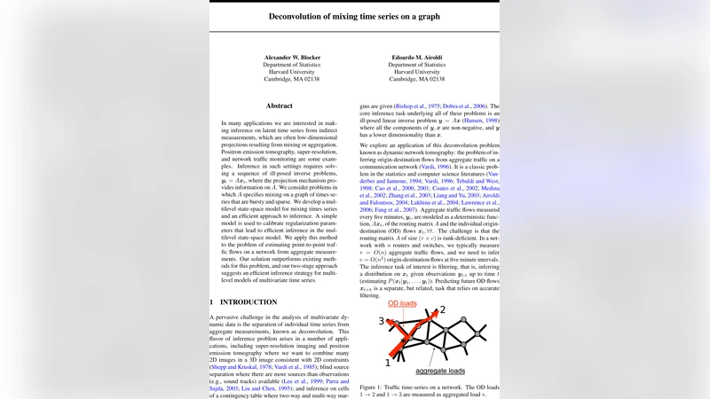
In many applications we are interested in making inference on latent time series from indirect measurements, which are often low-dimensional projections resulting from mixing or aggregation. Positron emission tomography, super-resolution, and network traffic monitoring are some examples. Inference in such settings requires solving a sequence of ill-posed inverse problems, y_t= A x_t, where the projection mechanism provides information on A. We consider problems in which A specifies mixing on a graph of times series that are bursty and sparse. We develop a multilevel state-space model for mixing times series and an efficient approach to inference. A simple model is used to calibrate regularization parameters that lead to efficient inference in the multilevel state-space model. We apply this method to the problem of estimating point-to-point traffic flows on a network from aggregate measurements. Our solution outperforms existing methods for this problem, and our two-stage approach suggests an efficient inference strategy for multilevel models of dependent time series.

💡 Research Summary

The paper tackles the classic inverse problem of recovering latent high‑dimensional time series from low‑dimensional aggregate observations, formalized as yₜ = A xₜ, where A is a known routing matrix that mixes origin‑destination (OD) traffic flows on a network graph. Because the number of OD pairs (c) far exceeds the number of observable link loads (r), the system is severely rank‑deficient and ill‑posed. Existing approaches—regularized least squares, EM‑based tomography, or simple Bayesian models—either ignore the bursty nature of network traffic or fail to enforce sparsity, leading to poor estimates.

Two‑stage modeling strategy
The authors propose a hierarchical (multilevel) state‑space model that captures two essential characteristics of real traffic: (1) burstiness—large, sudden spikes in volume—and (2) sparsity—many OD pairs are idle for long periods. The first layer models a latent intensity λᵢ,ₜ for each OD pair i as a log‑normal autoregressive process: log λᵢ,ₜ = ρ log λᵢ,ₜ₋₁ + εᵢ,ₜ, with εᵢ,ₜ ∼ N(θ₁ᵢ,ₜ, θ₂ᵢ,ₜ). This yields heavy‑tailed, temporally correlated dynamics. Conditional on λᵢ,ₜ, the actual flow xᵢ,ₜ follows a truncated Normal distribution with mean λᵢ,ₜ and variance λᵢ,ₜ τ (exp φₜ − 1), where φₜ is a global variance factor drawn from a Gamma prior. The truncation enforces non‑negativity and creates a point mass near zero, thereby inducing sparsity.

Calibration via a simple Gaussian SSM
Direct inference on the full hierarchical model is difficult because many regularization parameters (θ₁, θ₂, τ, etc.) are not identifiable from the data alone. To overcome this, the authors first fit a much simpler Gaussian state‑space model (linear AR(1) dynamics with additive Gaussian noise) to the observed aggregates yₜ. Using Kalman smoothing and maximum‑likelihood estimation, they obtain provisional estimates of the latent OD flows. These provisional flows are then projected onto the feasible polytope defined by A xₜ = yₜ and xₜ ≥ 0 using the iterative proportional fitting procedure (IPFP). From the smoothed series they compute empirical log‑differences and variances, which are used to set the hierarchical model’s θ₁ᵢ,ₜ and θ₂ᵢ,ₜ. This “coarse‑to‑fine” calibration supplies sensible regularization without manual tuning.

Sequential Monte Carlo (SIRM) inference
With calibrated hyper‑parameters, the hierarchical model is estimated using a Sample‑Importance‑Resample‑Move (SIRM) particle filter. Each particle contains the current intensity vector λₜ, the global variance φₜ, and the OD flow vector xₜ. The sampling step draws λₜ from its Gaussian transition, φₜ from its Gamma transition, and xₜ from the truncated Normal conditional on λₜ and φₜ. Because xₜ must satisfy the linear constraints A xₜ = yₜ and non‑negativity, the authors employ a Random Directions Algorithm (RDA) to propose feasible moves: they decompose A =