Simultaneous model-based clustering and visualization in the Fisher discriminative subspace

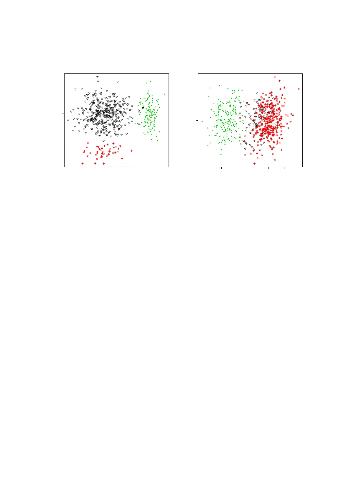
Sim ultaneous mo del-based clustering and visualiza tion in the Fisher discrim inativ e subspace Charles Bouveyr on 1 & Camille Br unet 2 1 Lab oratoire SAMM, EA 4543, Univ ersité Paris 1 P anth éon-Sorbonne 90 rue de T olbiac, 75013 P aris, F ra nce Email: charles.bouveyron@univ- paris1.fr 2 IBISC, T ADIB, FRE CNRS 3190, Univ ersité d’Evry V al d’Essonne 40 rue de Pel v oux, CE 1455, 91020 Evry Courcouronnes, F rance Email: camille.brunet@ibisc.univ- evry.fr Abstract Clustering in high-dimensional spaces is nowada y s a recur rent problem in ma ny sci- ent iﬁc domains but r emains a diﬃcult task from b oth the cluster ing accura cy and the result understanding p oints of view. This pa p er presents a discriminativ e laten t mixture (DLM) mo del which ﬁts the data in a la ten t or thonormal discriminative subspa ce with an in trinsic dimension lo w er than the dimension of the orig inal space. By constraining mo del parameter s within and b etw een groups, a family of 12 parsimonious DLM mo dels is exhibited which allows to ﬁt onto v ar ious situations. An estimation algorithm, called the Fisher-EM algo rithm, is also pro po sed for estimating bo th the mixture pa rameters and the discriminative subspace. Experiments on simulated and real datasets show that the propo sed approach per forms b etter than existing cluste r ing metho ds while providing a useful repr esentation o f the cluster ed da ta . The method is as well applied to the c lus - tering of ma ss sp ectro metr y data. Keyw ords: high-dimensional clustering, model-ba sed clustering, discriminative sub- space, Fisher criterion, visualization, parsimonious mo dels. 1 In tro duction In man y s cien tiﬁc domains, the measured observ ations are no wa da ys high-dimension al and clustering suc h data remains a c hallenging problem. Indeed, the most p opular clustering meth- o ds, whic h are based on the mixture model, show a disapp oin ting behavior in high-dimensional spaces. They suﬀer from the well-kno wn curse of di m ensionality [6] whic h is mainly due to the 1 fact that mo del-based clustering methods are o ver-param etrized in high-dimensiona l spaces. F urthermore, in severa l application s suc h as mass sp ectrometry or genomics, the num b er of a v ailable observ ations is small compared to the n um b er of v ariables and suc h a situation increases the diﬃcult y of the proble m. Hop efully , since the dimension of observ ed data is usually higher than their in trinsic dimen- sion, it is theoretically p ossible to reduce the dimension o f the original space without lo os ing an y information. Therefore, dimension reduction metho ds are traditionally us ed b efore the clustering step. F eature extraction metho ds suc h as principal comp onen t analysis (PCA) or feature selection methods are very p opular. How ev er, these approac hes of dimension reduction do not consider the classiﬁcation task and pro vide a sub-optimal data represen tation for the clustering step. Indeed, dimension reduction methods imply an informati on loss which could b e discriminativ e. Only few approac hes com bine dimension reduction with the classiﬁcation aim but, unfortunately , those approac hes are all sup ervised metho ds. Fisher discriminan t analysis (FDA) (see Chap. 4 of [28 ]) is one of them in the sup ervised classiﬁcation framew ork. FD A is a pow erful to ol for ﬁnding the subspace whic h b est discriminates the classes and re- v eals the structure of the data. This subspace is s panned b y the discriminativ e axes whic h maximize the ratio of the b et w een class and the within class v ariances. T o a void dimension reduction, sev eral s ubspace clustering metho ds ha v e b een prop osed in the past few yea rs to mo del the data of eac h group in lo w-dimensional subspaces. These methods turned out to b e very eﬃcien t in practice. Ho wev er, s ince these metho ds mo del eac h group in a s p eciﬁc subspace, they are not able to provide a global visualization of the clustered data whic h could b e helpful for the practitioner . Indeed, the clustering results of high-dimension al data are diﬃcult to understand without a v isualization of the clustered data. In addition, in scien tiﬁc ﬁelds suc h as genomics or economics, original v ariables hav e an actual meaning and the practitione r could b e interested in int erpreting the clustering results according to the v ariable meaning. In order to b oth ov ercome the curse of dimensionalit y and improv e the understanding of the clustering results, this w ork prop oses a method which adapts the traditional mixture mo del for mo deling and classifying data in a laten t discriminative subspace. F or this, the pro- p osed discriminativ e latent mixture (DLM) mo del com bines the mo del-based clustering goals with the discriminativ e criterion in tro duced b y Fisher. The estimation pro cedure prop osed in this pap er and named Fisher-EM has three main ob j ectiv es: ﬁrstly , it aims to impro ve clustering p erformances with the use of a discriminati v e subspace, secondly , it a voids estima- tion problems link ed to high dimensions through model parsimon y and, ﬁnally , it pro vides a lo w-dimensional discriminativ e represen tation of the clustered data. The reminder of this man uscript has the follo wing organization. Section 2 reviews the problem of high-dimen sional data clustering and ex is ting s olutions. Section 3 introduces the discriminativ e laten t mixture mo del and its submo dels. The link with existing approac hes is also discussed in Section 3. Section 4 presen ts an EM-based pro cedure, called Fisher-EM, f or 2 estimating the parameters of the DLM mo del. Initialization, mo del selection and con vergence issues are also considered in Section 4. In particular, the con vergenc e of the Fisher-EM algorithm has been pro v ed in this w ork only for one of the DLM models and the con vergence for the other mo dels should b e in ve stigated. In Section 5, the Fisher-EM algorithm is compared to existing clustering metho ds on simula ted and real datasets. Section 6 presen ts the application of the Fisher-EM algorithm to a real-w orld clustering problem in mass-sp ectromet ry imaging. Some concluding remarks and ideas for further works are ﬁnally given in Section 7 . 2 Related w orks Clustering is a tradit ional statistical prob lem whic h aims to divide a set of observ ations { y 1 , . . . , y n } described by p v ariables in to K homogeneous groups. The problem of clustering has b een widely studied for y ears and the reader could refer to [21, 30] for reviews on the clustering problem. Ho we v er, the in terest in clustering is still increasing s ince more and more scientiﬁ c ﬁelds require to cluster high-dimension al data. Moreo ver, suc h a task remains v ery diﬃcult s ince clustering methods suﬀer from the w ell-kno wn curse of dimensionality [6]. Con versely , the empty sp ac e phenomenon [48 ], whic h refers to the fact that high-dimensional data do not ﬁt the whole observ ation space but live in lo w-dimensional subspaces, giv es hop e to eﬃcien tly classify high-dimensional data. This section ﬁrstly reviews the framew ork of mo del-based clustering b efore exp osing the existing approach es to deal with the problem of high dimension in clustering. 2.1 Mo del-based clustering and high-dimensional data Mo del-based clustering, whic h has b een widely studied b y [21 , 40] in particular, aims to parti- tion observ ed data int o several groups whic h are mo deled separately . The o ver all population is considered as a mixture of these groups and most of time they are mo deled by a Gaus- sian structure. By considering a dataset of n observ ations { y 1 , . . . , y n } whic h is divided in to K homogeneous groups and by assuming that the observ ations { y 1 , ..., y n } are indep enden t realizations of a random v ector Y ∈ R p , the mixture model density is then: f ( y ) = K X k =1 π k f ( y ; θ k ) , (2.1) where f ( . ; θ k ) is often the mult iv ariate Gaussian density φ ( . ; µ k , Σ k ) parametr ized by a mean v ector µ k and a cov ariance matrix Σ k for the k th comp onen t. Unfortunately , mo del-based clustering metho ds sho w a disapp oint ing b eha vior when the num b er of observ ations is small compared to the n um b er of parameters to estimate. Indeed, in the case of the full Gaussian mixture mo del, the num b er of parameters to estimate is a function of the square of the dimension p and the estimation of this p oten tially large num b er of parameters is consequen tly diﬃcult with a small dataset. In particular, when the n umber of observ ations n is of the same 3 order than the num b er of dimensions p , most of the mo del-based clustering methods ha v e to face n umerical problems due to the ill-condit ioning of the co v ariance matric es. F urthermore, it is not p ossible to use the full Gaussian mixture mo del without restrictiv e ass umptions for clustering a dataset for whic h n is smaller than p . Indeed, for clustering suc h data, it w ould b e necessary to inv ert K cov ariance matrices whic h w ould b e singular. T o ov ercome these problems, sever al strategies ha v e b een prop osed in the literature among whic h dimension reduction and subspace clustering . 2.2 Dimension reduction and clustering Earliest approac hes prop osed to o vercom e the problem of high dimension in clustering b y reducing the dimension before using a traditional clustering metho d. Among the unsup ervised to ols of dimension reduction, PCA [32] is the traditional and certainly the most used tec hnique for dimension reduction. It aims to pro ject the data on a low e r dimensional subspace in whic h axes are built b y maximizing the v ariance of the pro jected data. Non-linear pro jection methods can also b e used. W e refer to [51] for a review on these alternativ e dimension reduction tec hniques. In a similar spirit, the generativ e top ographic mapping (GTM) [9] ﬁnds a non linear transformation of the data to map them on low-dim ensional grid. An other w a y to reduce the dimension is to s elect relev an t v ariables among the original v ariables. This problem has b een recen tly considered in the clustering con text by [10] and [36]. In [45 ] and [38 ], the problem of feature selection for mo del-based clustering is recasted as a mo del selection problem. Ho wev er, such approac hes remov e v ariables and consequen tly information whic h could ha ve b een discriminativ e for the clustering task. 2.3 Subspace clustering In the past f ew years, new approac hes fo cused on the mo deling of eac h group in sp eciﬁc subspaces of low dimensionalit y . Subspace clustering metho ds can b e split in to tw o cate- gories: heuristic and probabilistic metho ds. Heuristic metho ds us e algorithms to searc h for subspaces of high densit y within the original s pace. On the one hand, b ottom-up algorithms use histograms for selecting the v ariables whic h b est discriminate the groups. The Clique algorithm [1] w as one of the ﬁrst b ottom-up algorithms and remains a reference in this f amily of metho ds. On the other hand, top-do wn algorithms use iterativ e tec hniques whic h start with all original v ariables and remo v e at each iteration the dimensions without groups. A review on heuristic methods is a v ailable in [44]. Con versely , probabilistic metho ds assume that the data of each group liv e in a lo w-dimensional laten t s pace and usually mo del the data with a generativ e mo del. Earlier strategies [46] are bas ed on the f actor analysis mo del whic h assumes that the laten t space is related with the observ ation space through a linear relationship. Thi s mo del was recen tly extended in [5, 41] an d yields in particular the w ell kno wn mixture of probabilistic principal component analyzers [49]. Recen t wor ks [11, 42] 4 prop osed t wo families of parsimonious and regularized Gaussian mo dels whic h partially en- compass previous approac hes. All these tec hniques turned out to b e v ery eﬃcien t in practice to cluster high-dimensional data. How ev er, despite their qualities, these probabilistic metho ds mainly consider the clustering aim and do not tak e enough into accoun t the visualization and understanding asp ects. 2.4 F rom Fisher’s t heory t o discriminativ e clustering In the case of sup ervised classiﬁcation, Fisher p oses, in his precursor w ork [18], the problem of the discriminatio n of three sp ecies of iris described b y four measuremen ts . The main goal of Fisher wa s to ﬁnd a linear subspace that separates the clas ses according to a criterion (see [17] for more details). F or this, Fisher assumes that the dimensionalit y p of the original space is greater than the num b er K of classes. Fisher discriminan t analysis lo oks for a linear transformation U whic h pro jects the observ ations in a discriminativ e and low dimensional subspace of dimension d such that the linear transformation U of dimension p × d aims to maximize a criterion whic h is large when the b et w een-class co v ariance matrix ( S B ) is large and when the within-co v ariance matrix ( S W ) is small. Since the rank of S B is at most equal to K − 1 , the dimension d of the discriminativ e subspace is therefore at most equal to K − 1 as w ell. F our diﬀeren t criteria can b e found in the literature whic h satisfy such a constrain t (see [23] for a review). The criterion which is traditionally used is: J ( U ) = trace(( U t S W U ) − 1 U t S B U ) , (2.2) where S W = 1 n P K k =1 P i ∈ C k ( y i − m k )( y i − m k ) t and S B = 1 n P K k =1 n k ( m k − ¯ y )( m k − ¯ y ) t are resp ectiv ely the within and the b et w een co v ariance matrices, m k = 1 n k P K i ∈ C k y i is the em- pirical mean of the observ ed column vector y i in the class k and ¯ y = 1 n P K k =1 n k m k is the mean column v ector of the observ ations. The maximization of criterion (2.2) is eq uiv alent to the generalized eigen v alue problem [34]  S − 1 W S B − λI p  U = 0 and the classical solution of this problem is the eigen v ectors ass o ciated to the d largest eigen v alues of the matrix S − 1 W S B . F rom a practical p oin t of view, this optimization problem can also b e s olv ed using generalized eigen v alue solvers [24] in order to a void n umerical problems when S W is ill-conditio ned. Once the discriminativ e axes determined, linear discriminan t analys is (LDA) is usually applied to classify the data in to this subspace. The optimization of the Fisher criterion supp oses the non-singularit y of the matrix S W but it appears that the singularit y of S W o ccurs f requen tly , particularly in the case of ver y high-dimensional space or i n the case of under-sample d prob- lems. In the literature, diﬀeren t solutions [22, 23, 27 , 29, 31 ] are prop osed to deal with such a problem in a sup ervised classiﬁcation framew ork. In addition, since clustering approac hes are sensitiv e to high-dimensional and noisy data, recen t w orks [16, 35 , 15, 53] fo cused on comb in- ing lo w dimension al discriminativ e subspace with one of the most used clustering algorithm : k-means. Ho wev er, these approac hes do not really compute the discriminan t subspace and 5 are not in terested in the visualization and the understand ing of the data. 3 Mo del-based c lustering in a discrimi nativ e subspace This section in tro duces a mixture model, called the discriminativ e laten t mixture mo del, whic h aims to ﬁnd b oth a parsimonious and discriminativ e ﬁt for the data in order to generate a clustering and a visualization of the data. The mo deling prop osed in this section is mainly based on tw o key ideas: ﬁrstly , actual data are assumed to liv e in a laten t subspace with an in trinsic dimension low er than the dimension of the observ e d data and, secondly , a s ubspace of K − 1 dimensions is theoretic ally suﬃcien t to discriminate K groups. 3.1 The discriminativ e laten t mixture mo del Let { y 1 , . . . , y n } ∈ R p denote a dataset of n observ ations that one w ants to cluster in to K homogeneou s groups, i.e. adjoin to eac h observ ation y j a v alue z j ∈ { 1 , . . . , K } where z i = k indicates that the observ ation y i b elongs to the k th group. On the one hand, let us assume that { y 1 , . . . , y n } are indep endent observed realizations of a random vect or Y ∈ R p and that { z 1 , . . . , z n } are also indep enden t realizations of a random v ector Z ∈ { 1 , . . . , K } . On the other hand, let E ⊂ R p denote a latent s pace ass umed to b e the most discriminativ e subspace of dimension d ≤ K − 1 such that 0 ∈ E and where d is strictly lo we r than the dimension p of the observ ed space. Moreo ver, let { x 1 , . . . , x n } ∈ E denote the actual data, describ ed in the laten t space E of dimension d , whic h are in addition presumed to b e indep endent unobserv ed realizations of a random vector X ∈ E . Finally , for eac h group, the observ ed v ariable Y ∈ R p and the laten t v ariable X ∈ E are assumed to b e linke d through a linear transformation: Y = U X + ε, (3.1) where d < p , U is the p × d orthogonal matrix commo n to the K groups, suc h as U t U = I d , and ε ∈ R p , conditionally to Z , is a cen tered Gaussian noise term with co v ariance matrix Ψ k , for k = 1 , ..., K : ε | Z = k ∼ N ( 0 , Ψ k ) . (3.2) F ollo wing the classical framew ork of mo del-based clustering, eac h group is in addition assumed to b e distributed according to a Gaussian densit y function within the laten t space E . Hence, the random vector X ∈ E has the follo wing conditional densit y function: X | Z = k ∼ N ( µ k , Σ k ) , (3.3) where µ k ∈ R d and Σ k ∈ R d × d are resp ectively the mean and the co v ariance matrix of the k th group. Conditionally to X and Z , the random v ector Y ∈ R d has the follo wing conditional 6 distribution: Y | X, Z = k ∼ N ( U X , Ψ k ) , (3.4) and its marginal distribution is therefore a mixture of Gaussians: f ( y ) = K X k =1 π k φ ( y ; m k , S k ) , (3.5) where π k is the mixture proportion of the k th group and: m k = U µ k , S k = U Σ k U t + Ψ k , are resp ectiv ely the mean and the cov ariance matrix of the k th group in the observ ation space. Let us also deﬁne W = [ U, V ] a p × p matrix which satisﬁes W t W = W W t = I p and for whic h the p × ( p − d ) matrix V , is the orthonorma l complemen t of U deﬁned ab ov e. W e ﬁnally assume that the noise co v ariance matrix Ψ k satisﬁes the conditions V Ψ k V t = β k I d − p and U Ψ k U t = 0 d , suc h that ∆ k = W t S k W has the f ollo wing form: ∆ k =                Σ k 0 0 β k 0 . . . . . . 0 β k                     d ≤ K − 1            ( p − d ) This model, called the discriminativ e laten t mixture (DLM) mo del and referred to by DLM [Σ k β k ] in the sequel, is summarized b y Figure 1. The DLM [Σ k β k ] mo del is therefore parametrized b y the parameters π k , µ k , U , Σ k and β k , for k = 1 , ..., K and j = 1 , ..., d . On the one hand, the mixture prop ortions π 1 , ..., π K and the means µ 1 , ..., µ K parametrize in a classical w ay the prior probabilit y and the av erage laten t p osition of each group resp ectiv ely . On the other hand, U deﬁnes the laten t subspace E b y parametrizing its orien tation according to the basis of the original space. Finally , Σ k parametrize the v ariance of the k th group within the laten t subspace E whereas β k parametrizes the v ariance of this group outside E . With these nota- tions and f rom a practical p oin t of view, one can sa y that the v ariance of the actual data is therefore mo deled by Σ k and the v ariance of the noise is modeled b y β k . 7 P S f r a g r e p l a c e m e n t s X Y Z π = { π 1 , ..., π K } µ k ∈ E Σ k W = [ U, V ] ε Ψ k Figure 1: Graphical s ummary of the DLM [Σ k β k ] mo del 3.2 The submo dels of the D LM [Σ k β k ] mo del Starting with the DLM [Σ k β k ] mo del presen ted in the previous paragraph, sev eral submo dels can b e generated b y applying constrain ts on parameters of the matrix ∆ k . F or instance, the co v ariance matrices Σ 1 , . . . , Σ K in the laten t space can b e assumed to b e common across groups and this s ubmo del will b e referred to by DLM [Σ β k ] . Similarl y , in eac h group, Σ k can b e assumed to b e diagonal, i.e. Σ k = d iag ( α k 1 , . . . , α k d ) . This submo del will b e referred to by DLM [ α kj β k ] . In the s ame manner, the p − d last v alues of ∆ k can b e ass umed to b e common for the k classes, i.e. β k = β , ∀ k = 1 , ..., K , meaning that the v ariance outside the discriminan t subspace is common to all groups. This assumption can b e view ed as mo deling the noise v ariance with a unique parameter whic h seems natural for data obtained in a common acquisition pro cess. F ollow ing the notation sys tem introduces ab ov e, this submo del will b e referred to by DLM [ α kj β ] . T he v ariance within the laten t subspace E can also b e ass umed to b e isotropic f or eac h group and the asso ciated submo del is DLM [ α k β k ] . In this case, the v ariance of the data is ass umed to b e isotropic b oth within E and outside E . Simil arly , it is p ossible to constrain the previous mo del to ha ve the parameters β k common b et w een classes and this gives rise to the mo del DLM [ α k β ] . Finally , the v ariance within the subspace E can b e assumed to be indep enden t from the mixture component and this corresp onds to the mo dels DLM [ α j β k ] , DLM [ α j β ] , DLM [ αβ k ] and DLM [ αβ ] . W e therefore enume rate 12 diﬀeren t DLM mo dels and an ov erview of them is prop osed in T able 1 . The table also gives the maxim um n um b er of free parameters to estimate (case of d = K − 1 ) according to K and p for the 12 DLM mo dels and for some classical mo dels. The F ull-GMM mo del refers to the classical Gaussian mixture mo del with full co v ariance matrices, the Com-GMM model refers to the Gaussian mixture mo del for whic h the cov ariance matrices are assumed to b e equal to a common co v ariance matrix ( S k = S , ∀ k ), Diag-GMM refers to the Gaussian mixture mo del 8 Mo del Nb. of parameters K = 4 and p = 100 DLM [Σ k β k ] ( K − 1) + K ( K − 1) + ( K − 1)( p − K/ 2) + K 2 ( K − 1) / 2 + K 337 DLM [Σ k β ] ( K − 1) + K ( K − 1) + ( K − 1)( p − K/ 2) + K 2 ( K − 1) / 2 + 1 334 DLM [Σ β k ] ( K − 1) + K ( K − 1) + ( K − 1)( p − K/ 2) + K ( K − 1) / 2 + K 319 DLM [Σ β ] ( K − 1) + K ( K − 1) + ( K − 1)( p − K/ 2) + K ( K − 1) / 2 + 1 316 DLM [ α kj β k ] ( K − 1) + K ( K − 1) + ( K − 1)( p − K / 2) + K 2 325 DLM [ α kj β ] ( K − 1) + K ( K − 1) + ( K − 1)( p − K/ 2) + K ( K − 1) + 1 322 DLM [ α k β k ] ( K − 1) + K ( K − 1) + ( K − 1)( p − K / 2) + 2 K 317 DLM [ α k β ] ( K − 1) + K ( K − 1) + ( K − 1)( p − K/ 2) + K + 1 314 DLM [ α j β k ] ( K − 1) + K ( K − 1) + ( K − 1)( p − K/ 2) + ( K − 1) + K 316 DLM [ α j β ] ( K − 1) + K ( K − 1) + ( K − 1)( p − K/ 2) + ( K − 1) + 1 313 DLM [ αβ k ] ( K − 1) + K ( K − 1) + ( K − 1)( p − K/ 2) + K + 1 314 DLM [ αβ ] ( K − 1) + K ( K − 1) + ( K − 1)( p − K/ 2) + 2 311 F ull-GMM ( K − 1) + K p + K p ( p + 1) / 2 20603 Com-GMM ( K − 1) + K p + p ( p + 1) / 2 5453 Mixt-PPCA ( K − 1) + K p + K ( d ( p − ( d + 1) / 2) + d + 1) + 1 1198 ( d = 3 ) Diag-GMM ( K − 1) + K p + K p 803 Sphe-GMM ( K − 1) + K p + K 407 T able 1: Num b er of free parameters to estimate when d = K − 1 for the DLM mo dels and some classical mo dels (see text for details). 9 for whic h S k = diag( s 2 k 1 , ..., s 2 k p ) with s 2 k ∈ R p and Sphe-GMM refers to the G auss ian mixture mo del for which S k = s 2 k I p with s 2 k ∈ R . Finally , Mixt-PPCA denotes the subspace clustering mo del proposed b y Tipping and Bishop in [49]. In addition to the nu m b er of free parameters to estimate, T able 1 give s this n umber for sp eciﬁc v alues of K and p in the righ t column. The n umber of free parameters to estimate giv en in the cen tral column can b e decomposed in the n umber of parameters to estimate for the prop ortions ( K − 1 ), for the means ( K p ) and for the co v ariance matrices (last terms). Among the classical m o dels, the F ull-GMM mo del is a highly parametrized model and requires the estimation of 20603 parameters when K = 4 and p = 100 . Con v ersely , the Diag-GMM and Sphe-GMM mo del are very parsimonious mo dels since they resp ectiv ely require the estimation of only 803 and 407 parameters when K = 4 and p = 100 . The Com-GMM and Mixt-PPCA mo dels app ear to b oth ha ve an intermed iate complexit y . How ev er, the Mixt-PPCA mo del is a less constrained mo del compared to the Diag-GMM mo del and should b e preferred for clustering high-dimensional data. Finally , the DLM mo dels turn out to hav e a lo w complexit y whereas their mo deling capacit y is compar able to the one of the Mixt-PPCA mo del. In addition, the complexit y of the DLM mo dels dep ends only on K and p whereas the Mixt-PPCA mo del dep ends from an h yp er-parameter d . 3.3 Links wit h existing mo dels A t this p oin t, s ome links can b e established with mo dels existing in the clustering literature. The closest mo dels ha ve b een prop osed in [5], [11] and [42 ] and are all derived f rom the mixture of factor analyzer (MF A) mo del [41, 46]. First, in [11 ], the authors prop osed a family of 28 parsimonious and ﬂexible Gaussian mo dels ranging from a very general mo del, referred to as [ a k j b k Q k d k ] , to very s imple mo dels. Com pared to the standard MF A mo del, these parsimonious mo dels assume that the noise v ariance is isotropic. In particular, this w ork can b e view ed as an extension of the mixture of principal comp onen t analyzer (Mixt- PPCA) mo del [49]. Among this f amily of parsimonious mo dels, 14 mo dels assume that the orien tation of the group-sp eciﬁc subspaces is common (common Q k ). The f ollowin g year, McNic holas and Murph y [42] prop osed as w ell a family of 8 parsimonious Gaussian mo dels b y extending the MF A model b y constraining the loading and error v ariance matrices across groups. In this w ork, the noise v ariance can b e is otropic or not. Let us remark that the t wo f amilies of parsimonious Gaussian mo dels s hare some mo d els: for instance, the mo del UUC of [42] corresponds to the mo del [ a k j b k Q k d ] of [11]. Among the 8 parsimonious mo dels presen ted in [42], 4 mo dels ha ve the loading matrices constrained across the groups. More recen tly , Beak et al. [5] prop osed as well a MF A mo del with a common loading matrix. I n this case, the noise v ariance is not constrained. Despite their diﬀerences, all these parsimonious Gaussian mo dels share the assumption that the group subspaces ha ve a comm on orien tation and are therefore close to the DLM mo dels presen ted in this w o rk. Ho w ever, these mo dels with common loadings c ho ose the orien tation suc h as the v ariance of the pro jected data is maxim um whereas the DLM mo dels choose the laten t subspace orient ation s uc h as it b est 10 discriminates the groups. This sp eciﬁc feature of the DLM mo dels should therefore impro ve in most cases b oth the clustering and the vis ualization of the results. In particular, the DLM mo dels should b e able to b etter mo del situations where the axes carrying the greatest v ariance are not parallel to the discriminativ e axes than the other approac hes (Figure 10.1 of [23] illustrates s uch a situation). 4 P arameter estimati on: the Fi sher-EM algorithm Since this w ork fo cuses on the clustering of unlab eled data, this section in tro duces an esti- mation procedure whic h adapts the traditional EM algorithm for estimating the paramete rs of DLM mo dels presen ted in the previous section. Due to the nature of the mo dels describ ed ab o ve, the Fisher-EM algorithm alternat es b et wee n three steps: • an E s tep in whic h p osterior probabi lities that observ ations b elong to the K groups are computed, • a F step whic h estimates the orien tation matrix U of the discriminativ e laten t s pace conditionally to the posterior probabili ties, • a M step in whic h paramete rs of the mixture mo del are estimated in the laten t subspace b y maximizin g the conditional exp ectation of the complete likelih o o d. This estimation pro cedure relativ e to the DLM mo dels is called herea fter the Fisher-EM algorithm. W e chose to name this estimation pro cedure after Sir R . A. Fisher since the ke y idea of the F step comes from his famous w ork on discriminati on. The remainde r of this section details the simple form of this procedure. Let us ho w ev er notice that the Fisher-EM algorithm can b e also used in com bination with the sto ch astic [13] and classiﬁcation v ersions [14] of the EM algorithm. 4.1 The E st ep This step aims to compute, at iteration ( q ) , the ex p ectation of the complete log-lik eliho o d conditionally to the curren t v alue of the parameter θ ( q − 1) , whic h, in practice , reduces to the computation of t ( q ) ik = E [ z ik | y i , θ ( q − 1) ] where z ik = 1 if y i comes from the k th comp onen t and z ik = 0 otherwise. Let us also recall that t ( q ) ik is as w ell the p osterior probabilit y that the observ ation y i b elongs to the k th comp onent of the mixture. The f ollowin g prop osition pro vides the explicit f orm of t ( q ) ik , f or i = 1 , ..., n , k = 1 , ..., K , in the case of the mo del DLM [Σ k β k ] . Demonstration of this result is detailed in App endix A.1. Prop osition 1. With the assumption s of the mo del DLM [Σ k β k ] , the p osterior pr ob abiliti es t ( q ) ik , 11 i = 1 , ..., n , k = 1 , ..., K , c an b e expr esse d as : t ( q ) ik = 1 P K l =1 exp  1 2 (Γ ( q − 1) k ( y ) − Γ ( q − 1) l ( y ))  , (4.1) with: Γ ( q − 1) k ( y i ) = || P ( y i − m ( q − 1) k ) || 2 D k + 1 β ( q − 1) k || ( y i − m ( q − 1) k ) − P ( y i − m ( q − 1) k ) || 2 + log     Σ ( q − 1) k     + ( p − d ) log ( β ( q − 1) k ) − 2 log ( π ( q − 1) k ) + γ , (4.2) wher e || . || 2 D k is a norm on the latent sp ac e E deﬁne d by || y || 2 D k = y t D k y , D k = ˜ W ∆ − 1 k ˜ W t , ˜ W is a p × p matri x c ontainin g the d ve ctors of U ( q − 1) c omplete d by zer os such as ˜ W = [ U ( q − 1) , 0 p − d ] , P is the pr oje ction op er ator on the latent sp ac e E , i.e. P ( y ) = U ( q − 1) U ( q − 1) t y , and γ = p log (2 π ) is a c onstant term. Besides its compu tational in terest, Prop osition 1 pro vides as w ell a comprehensiv e in ter- pretation of the cost function Γ k whic h mainly go v erns the computation of t ik . Indeed, it app ears that Γ k mainly dep ends on tw o distances: the distance b et w een the pro jections on the discriminan t subspace E of the observ ation y i and the mean m k on the one hand, and, the distance b et w een the pro j ections on the complemen tary s ubspace E ⊥ of y i and m k on the other hand. Remark that the latter distance can b e reform ulated in order to a void the us e of the pro jection on E ⊥ . Indeed, as Figure 2 illustrates, this distance can b e re-express ed ac- cording pro jections on E . Therefore, the p os terior probabilit y t ik = P ( z ik = 1 | y i ) will b e close to 1 if b oth the distances are small whic h s eems quite natural. Ob viously , these distances are also balanced by the v ariances in E and E ⊥ and b y the mixture prop ortions. F urthermore, the fact that the E step do es not require the use of the pro jection on the complemen tary subspace E ⊥ is, from a computational p oint of view, v ery important b ecause it will provide the stabilit y of the algorithm and will allo w its use when n ≪ p ( cf. paragraph 4.6). 4.2 The F step This step aims to determina te, at iteration ( q ) , the discriminativ e laten t subspace of dimension d ≤ K − 1 in whic h the K groups are b est separated. Naturally , the estimation of this laten t subspace has to b e done conditionally to the curren t v alues of p osterior probabilities t ( q ) ik whic h indicates the curren t soft partition of the data. Estimating the discriminativ e laten t subspace E ( q ) reduces to the computation of d discriminativ e axes. F ollo wing the original idea of Fisher [18], the d axes whic h b est discriminate the K groups are those whic h maximize the traditional criterion J ( U ) = tr (( U t S W U ) − 1 U t S B U ) . H ow ev er, the traditional criterion J ( U ) assume that the data are complete (sup ervised classiﬁcation framew ork). Unfortunately , the situation of intere st here is that of unsup ervised classiﬁcation and the matrices S B and S W ha ve therefore to b e deﬁned conditionally to the curren t sof t partition. F urthermore, the 12 0 P S f r a g r e p l a c e m e n t s m 1 m 2 µ 1 x y E E ⊥ Figure 2: T w o groups and their 1 -dimension al discriminativ e subspace. DLM mo dels as s ume that the discriminativ e laten t subspace m ust ha ve an orthono rmal basis and, sadly , the traditional Fisher’s approac h pro vides non-orthogonal discriminativ e axes. T o o verc ome b oth problems, this paragraph prop oses a pro cedure which k eeps the key idea of Fisher while pro viding orthonormal discriminativ e axes conditionally to the curren t soft partition of the data. The pro cedure follows the concept of the orthonormal discriminan t v ector (OD V ) method introduced b y [19] in the s up ervised case and then extended b y [25 , 26, 37, 52], whic h s equen tially selects the most discriminative features in maximizing the Fisher criterion sub ject to the orthogonalit y of features. First, it is necessary to in tro duce the soft b et ween-c o v ariance matrix S ( q ) B and the soft within-co v ariance matrix S ( q ) W . The soft b et w een- co v ariance matrix S ( q ) B is deﬁned conditionally to the p osterior probab ilities t ( q ) ik , obtained in the E step, as follo ws: S ( q ) B = 1 n K X k =1 n ( q ) k ( ˆ m ( q ) k − ¯ y )( ˆ m ( q ) k − ¯ y ) t , (4.3) where n ( q ) k = P n i =1 t ( q ) ik , ˆ m ( q ) k = 1 n P n i =1 t ( q ) ik y i is the soft mean of the k th group at iteration q and ¯ y = 1 n P n i =1 y i is the empirical mean of the whole dataset. Since the relation S = S ( q ) W + S ( q ) B holds in this context as w ell, it is preferable from a computational p oin t of v iew to use the co v ariance matrix S = 1 n P n i =1 ( y i − ¯ y )( y i − ¯ y ) t of the whole dataset in the maximization problem instead of S ( q ) W since S remains ﬁxed o v er the iteration. The F step of the Fisher-EM 13 therefore aims to solv e the follo wing optimiza tion problem:    max U trace  ( U t S U ) − 1 U t S ( q ) B U  , wrt u t j u l = 0 , ∀ j 6 = l ∈ { 1 , . . . , d } , (4.4) where u j is the j th column vector of U . F ollo wing the OD V pro cedure, the d axes solution of this optimization problem are iterativ ely constructed by , ﬁrst, computing an orthogonal complemen tary s ubspace to the curren t set of discriminativ e axes and, then, maximizing the Fisher criterion in this orthogonal subspace b y solving the asso ciated generalized eigen v alue problem. T o initialize this iterative pro cedure, the ﬁrst ve ctor of U is therefore the eigen- v ector asso ciated with the largest eigen v alue of the matrix S − 1 S ( q ) B . Then, assuming that the r − 1 ﬁrst orthonormal discriminativ e axes { u 1 , . . . , u r − 1 } , whic h span the space B r − 1 , ha ve b een computed, the r th discriminativ e axis has to lie in the subspace B ⊥ r − 1 orthogonal to the space B r − 1 . The Gram-Sc hmidt orthonormalizatio n pro cedure allow s to ﬁnd a basis V r = { v r , v r +1 , ..., v d } for the orthogonal subspace B ⊥ r − 1 suc h that: v l = α l ( I ℓ − 1 − ℓ − 1 X j =1 v j v t j ) ψ l , ℓ = r , . . . , p (4.5) where v j = u j for j = 1 , ..., r − 1 , α ℓ is normalization constan t s uc h that || u ℓ || = 1 and ψ ℓ is a v ector linearly independen t of u j ∀ j ∈ { 1 , . . . , ℓ − 1 } . Then, the r th discriminativ e axis is giv en b y: u r = P r − 1 u max r || u max r || , (4.6) where P r − 1 is the pro jector on B r − 1 , u max r is the eigenv ector asso ciated with the largest eigen v alue of the matrix S − 1 r S ( q ) B r with: S r = V r t S V r , S ( q ) B r = V r t S ( q ) B V r , i.e. S r and S ( q ) B r are resp ectivel y the co v ariance and soft b et ween -co v ariance matrices of the data pro jected int o the orthogona l subspace B ⊥ r − 1 . This iterativ e pro cedure stops when the d orthonormal discriminativ e axes u j are computed. 4.3 The M step This third step estimates the mo del parameters by maximizing the conditional exp ectation of the complete lik eliho o d. The f ollo wing proposition pro vides the expression of the conditional exp ectation of the complete log-lik eliho o d in the case of the DLM [Σ k β k ] mo del. A pro of of this result is provide d in App endix A.2 14 Prop osition 2. In the c ase of the mo del DLM [Σ k β k ] , the c onditional exp e ctation of c omplete lo g-likeliho o d Q ( y 1 , . . . , y n , θ ) has the fol lowing expr ession: Q ( y 1 , . . . , y n , θ ) = − 1 2 K X k =1 n k h − 2 log( π k ) + trace(Σ − 1 k U t C k U ) + log( | Σ k | ) + ( p − d ) log ( β k ) + 1 β k   trace( C k ) − d X j =1 u t j C k u j   + γ i . (4.7) wher e C k is the empiric al c ovarianc e matrix of the k th gr oup, u j is the j th c olumn ve ctor of U , n k = P n i =1 t ik and γ = p log(2 π ) is a c onstant term. A t iteration q , the maximization of Q conduces to an estimation of the mixture prop ortions π k and the means µ k for the K comp onen ts by their empirical coun terparts: ˆ π ( q ) k = n k n , ˆ µ ( q ) k = 1 n k n X i =1 t ( q ) ik U ( q ) t y i , where n k = P n i =1 t ( q ) ik and U ( q ) con tains, as columns vect ors, the d discriminativ e axes u ( q ) j , j = 1 , ..., d , pro v ided b y the F step at iteration q . The f ollo wing prop osition provides estimates for the remaining parameters for the 12 DLM mo dels whic h ha v e to b e up dated at each iteration of the FEM procedure. Pro ofs of the follo wing results are given in App endix A.2. Prop osition 3. At iter ation q , the estimates for varianc e p ar ameters of the 12 DLM mo dels ar e: • Mo del DLM [Σ k β k ] : ˆ Σ ( q ) k = U ( q ) t C ( q ) k U ( q ) , ˆ β ( q ) k = trace( C ( q ) k ) − P d j =1 u ( q ) t j C ( q ) k u ( q ) j p − d , (4.8) • Mo del DLM [Σ k β ] : ˆ Σ ( q ) k = U ( q ) t C ( q ) k U ( q ) , ˆ β ( q ) = trace( C ( q ) ) − P d j =1 u ( q ) t j C ( q ) u ( q ) j p − d , (4.9) • Mo del DLM [Σ β k ] : ˆ Σ ( q ) = U ( q ) t C ( q ) U ( q ) , ˆ β ( q ) k = trace( C ( q ) k ) − P d j =1 u ( q ) t j C ( q ) k u ( q ) j p − d , (4.10) 15 • Mo del DLM [Σ β ] : ˆ Σ ( q ) = U ( q ) t C ( q ) U ( q ) , ˆ β ( q ) = trace( C ( q ) ) − P d j =1 u ( q ) t j C ( q ) u ( q ) j p − d , (4.11) • Mo del DLM [ α kj β k ] : ˆ α ( q ) k j = u ( q ) t j C ( q ) k u ( q ) j , ˆ β ( q ) k = trace( C ( q ) k ) − P d j =1 u ( q ) t j C ( q ) k u ( q ) j p − d , (4.12) • Mo del DLM [ α kj β ] : ˆ α ( q ) k j = u ( q ) t j C ( q ) k u ( q ) j , ˆ β ( q ) = trace( C ( q ) ) − P d j =1 u ( q ) t j C ( q ) u ( q ) j p − d , (4.13) • Mo del DLM [ α k β k ] : ˆ α ( q ) k = 1 d d X j =1 u ( q ) t j C ( q ) k u ( q ) j , ˆ β ( q ) k = trace( C ( q ) k ) − P d j =1 u ( q ) t j C ( q ) k u ( q ) j p − d , (4.14) • Mo del DLM [ α k β ] : ˆ α ( q ) k = 1 d d X j =1 u ( q ) t j C ( q ) k u ( q ) j , ˆ β ( q ) = trace( C ( q ) ) − P d j =1 u ( q ) t j C ( q ) u ( q ) j p − d , (4.15) • Mo del DLM [ α j β k ] : ˆ α ( q ) j = u ( q ) t j C ( q ) u ( q ) j , ˆ β ( q ) k = trace( C ( q ) k ) − P d j =1 u ( q ) t j C ( q ) k u ( q ) j p − d , (4.16) • Mo del DLM [ α j β ] : ˆ α ( q ) j = u ( q ) t j C ( q ) u ( q ) j , ˆ β ( q ) = trace( C ( q ) ) − P d j =1 u ( q ) t j C ( q ) u ( q ) j p − d , (4.17) • Mo del DLM [ αβ k ] : ˆ α ( q ) = 1 d d X j =1 u ( q ) t j C ( q ) u ( q ) j , ˆ β ( q ) k = trace( C ( q ) k ) − P d j =1 u ( q ) t j C ( q ) k u ( q ) j p − d , (4.18) 16 • Mo del DLM [ αβ ] : ˆ α ( q ) = 1 d d X j =1 u ( q ) t j C ( q ) u ( q ) j , ˆ β ( q ) = trace( C ( q ) ) − P d j =1 u ( q ) t j C ( q ) u ( q ) j p − d , (4.19) wher e the ve ctors u ( q ) j ar e the discriminati ve axes pr ovide d by the F step at iter ation q , C ( q ) k = 1 n ( q ) k P n i =1 t ( q ) ik ( y i − ˆ m ( q ) k )( y i − ˆ m ( q ) k ) t is the soft c ovarianc e matrix of the k th gr oup, ˆ m ( q ) k = 1 n P n i =1 t ( q ) ik y i and ﬁnal ly C = 1 n P K k =1 n k C k is the s oft within -c ovarianc e matri x of the K gr oups. 4.4 Initialization and mo del selection Since the Fisher-EM pro cedure presen ted in this wo rk b elongs to the family of EM-based algorithms, the Fisher-EM algorithm can inherit the most eﬃcient s trategies for initialization and mo del selection from previous w orks on the EM algorithm. Initialization Although the EM algorithm is widely used, it is also w ell-kno wn that the p erformance of the algorithm is link ed to its initial conditions. Sev eral strategies hav e b een prop osed in the literature for initializi ng the EM algorithm. A p opular practice [8] executes the EM algorithm sev eral times from a random initialization and keep only the set of parameters asso ciated with the highest likelih o o d. The use of k-means or of a random partition are also standard approac hes for initializing the algorithm. McLac hlan and P eel [40] ha ve also prop osed an initialization through the parameters b y generating the mean and the co v ariance matrix of each mixture comp onent from a multiv ariate normal distribution parametrize d b y the empirical mean and empirical co v ariance matrix of the data. In practice, this latter initialization pro cedure w orks well but, unfortunately , i t cannot b e applied directly to the Fisher-EM algorithm since mo del parameters live in a space diﬀeren t from the observ ation space. A simple w ay to adapt this strategy could b e to ﬁrst determine a laten t space using PCA and then s im ulate mixture parameters in this initialization laten t space. Mo del selec tion In mo del-based clustering, it is frequent to consider several mo dels in order to ﬁnd the most appropriate mo del for the considered data. Since a mo del is deﬁned b y its num b er of componen t K and its parametrizat ion, mo del selection allo ws to b oth select a parametrizat ion and a n umber of comp onen ts. Several criteria for model selection ha v e been prop osed in the literature and the famous ones are p enalized likelihoo d criteria. Classical to ols for mo del selection include the AI C [2 ], BIC [47] and ICL [7] criteria. The Ba yesian Information Criterion (BIC) is certainly the most p opular and consists in selecting the mo del whic h p enalizes the likelihoo d b y γ ( M ) 2 log( n ) where γ ( M ) is the n umber of parameters in mo del M and n is the n um b er of observ ations. On the other hand, the AIC criterion p enalizes 17 the log-likelih o o d by γ ( M ) whereas the ICL criterion add the p enalt y P n i =1 P K k =1 t ik log( t ik ) to the one of the BIC criterion in order to fav or w ell separated models. The v alue of γ ( M ) is of course sp eciﬁc to the mo del selected b y the practitioner ( cf . T able 1). In the exp erimen ts of the follo wing s ections, the BI C criterion is used b ecause of its p opularit y but the ICL criterion should also b e w ell adapted in our conte xt. 4.5 Computational asp ects As all iterativ e pro cedures, the con vergen ce, the stopping criterion and the computational cost of the Fisher-EM algorithm deserv e to b e discussed. Con vergence Alth ough the Fisher-EM algorithm presen ted in the previous paragraphs is an EM-lik e algorithm, it do es not satisfy at a ﬁrst glance to all conditions required b y the con verg ence theory of the EM algorithm. Indeed, the update of the orien tation matrix U in the F step is done b y maximizing the Fisher criterion and not b y directly maximizing the exp ected complete log-like liho o d as required in the EM algorithm theory . F rom this p oin t of view, the con vergen ce of the Fisher-EM algorithm cannot therefore b e guaran teed. H o wev er, as demonstrated b y Campb ell [12] in the sup ervised case and by Celeux and Gov aert [14] in the unsup ervised case, the maximization of the Fisher criterion is equiv alen t to the maximization of the complete lik elihoo d when all mixture comp onen ts ha ve the same diagonal co v ariance matrix ( S k = σ 2 I p for k = 1 , ..., K ). In our mo del, by considering the homoscedastic case with a diagona l co v ariance matrix, the conditional exp ectation of the complete log-lik eliho o d can b e rewritten as − n 2 h trace   U t S U  − 1  U t W U  i + γ where γ is a constan t term according to U . Hence, with these assumptions, maximizing this criterion according to U is equiv alen t to minimizing the Fis her criterion trace   U t S U  − 1  U t W U   . Consequen tly , f or the model DLM [ αβ ] whic h assumes the equality and the diagonalit y of co v ariance matrices, the F step of the Fisher-EM algorithm satisﬁes the con v ergence conditions of the EM algorithm theory and the conv ergence of the Fisher-EM algorithm can b e guaran teed in this case. F or the other DLM mo dels, although the conv ergence of the Fisher-EM pro cedure cannot b e guaran teed, our practical exp erience has shown that the Fisher-EM algorithm rarely fails to conv erge with these mo dels if correctly initialized. Stopping cri terion and con ve rgence monitoring T o decide whether the algorithm has con verg ed or not, w e prop os e to use the Aitken ’s criterion [39]. This criterion estimates the asymptotic maxim um of the log-lik elihoo d in order to detect in adv ance the algorithm con ver- gence. Indeed, the con vergen ce of the EM algorithm can b e sometimes slo w in practice due to its linear conv ergence rate and it is often not necessary to wa it for the actual con v ergence to obtain a goo d parameter estimate under standard conditions. At iteration q , the A itk en’s criterion is deﬁned by A ( q ) =  ℓ ( q + 1) − ℓ ( q )  /  ℓ ( q ) − ℓ ( q − 1)  where ℓ ( q ) is the log-lik elihoo d 18 v alue at iteration q . Then, asymptotic estimate of the log-likelih o o d maxim um is given b y: ℓ ( q + 1) ∞ = ℓ ( q ) + 1 1 − A ( q )  ℓ ( q + 1) − ℓ ( q )  , (4.20) and the algorithm can b e considered to ha ve conv erged if    ℓ ( q + 1) ∞ − ℓ ( q ) ∞    is smaller than a small p ositiv e n um b er (pro vided b y the us er). In practice, if the criterion is not satisﬁed after a maxim um num b er of iterations (provided b y the user as w ell), the algorithm stops. Afterw ard, it is p ossible to c hec k whether the provide d estimate is a lo cal maximu m by computing the Hes sian matrix (using ﬁnite diﬀeren tiation) whic h should b e negativ e deﬁnite. In the exp erimen ts presen ted in the followi ng section, the con v ergence of the Fisher-EM algorithm has b een c hec ked using suc h an approac h. Computational cost Ob viously , since the additional F step is iterativ e, the computational complexit y of the Fis her-EM pro cedure is somewhat bigger than the one of the ordinary EM algorithm. The F step requires d ( d − 2) / 2 iterations due to the Gram-Sc hmidt procedure used for the orthogonalization of U . How ever, since d is at most equal to K − 1 and is supp osed to b e small compar ed to p , the complexit y of the F step is not a quadratic function of the data dimension whic h could b e large. F urthermore, it is imp ortant to notice that the complexit y of this s tep do es not dep end on the n umber of observ ations n . Although the prop osed algorithm is more time consuming than the usual EM algorithm, it is altogether actually us able on recen t PCs even for large scale problems. Indeed, w e ha v e observ ed on simulati ons that Fisher-EM app ears to b e 1 . 5 times s low er on a verag e than EM (with a diagonal mo del). As an example, 24 s econds are on a verag e necessary for Fisher-EM to cluster a dataset of 1 000 observ ations in a 100 -dimensional space whereas EM requires 16 seconds. 4.6 Practical asp ects The DLM mo dels, f or whic h the Fis her-EM algorithm has b een prop osed as an estimation pro cedure, presen ts several practical and n umerical inte rests among which the abilit y to vi- sualize the clustered data, to inte rpret the discriminativ e axes and to deal with the so-called n ≪ p problem. Choice o f d and visualization in the discri minativ e sub space The prop osed DLM mo dels are all parametrize d by the intr isinc dimension d of the discriminativ e laten t subspace whic h is theoretically at most equal to K − 1 . Even though the actual v alue of d is strictly smaller than K − 1 for the dataset at hand, w e recommand in practice to set d = K − 1 when n umerically p ossible in order to av oid stabilit y problems with the Fisher-EM algorithm. F urthermore, it is alwa y s b etter to extract more discriminativ e axes than to miss relev ant dimensions and K − 1 is often in practice a small v alue compared to p . Besides, a natural use of the discriminativ e axes ma y certainly b e the visualization of the clustered data. Indeed, it 19 is no w ada ys clear that the v is ualization help h uman op erators to understand the results of an analysis. With the Fisher-EM algorithm, it is easy to pro ject and visualize the cluster data in to the estimated discriminativ e laten t subspace if K ≤ 4 . When K > 4 , the actual v alue of d can b e estimated b y lo oking at the eigen v alue scree of S − 1 W S B and t wo cases hav e therefore to b e considered. On the one hand, if the estimated v alue of d is at most equal to 3 , the practitioner can therefore vis ualize his data b y pro jecting them on the d ﬁrst discriminativ e axes and no discriminativ e information loss is to b e deplored in this case. On the other hand, if the estimated v alue of d is strictly larger than 3 , the visualization b ecomes ob viously more diﬃcult but the practitioner ma y simply use the 3 ﬁrst discriminativ e axes whic h are the most discriminativ e ones among the K − 1 pro vided axes. Let us ﬁnally notice that the visualization qualit y is of course related to the clustering quality . Indeed, the visualization pro v ided b y the Fisher-EM algorithm may b e disapp ointi ng if the clustering results are p o or, due to a bad initialization for instance. A goo d solution to a v oid such a situation ma y be to initialize the Fisher-EM algorithm with the “mini-EM” strategy or with the results of a classical EM algorithm. In terpretation of t he discriminativ e axes Bey ond the natural in terest of vis ualization, it ma y also b e usef ul from a practical p oint of view to in terpret the estimated discriminativ e axes, i.e. u 1 , ..., u d with the notations of the previous sections. The main in terest for the practitioner would b e to ﬁgure out whic h original dimensions are the most discriminativ e. This can b e done by lo oking at the matrix U whic h conta ins u 1 , ..., u d as column vec tors. In the classical framew ork of factor analysis, this matrix is k no wn as the loading matrix (the discriminativ e axes u 1 , ..., u d are the loadings). Th us, it is p ossible to ﬁnd the most discriminativ e original v ariables by selecting the highes t v alues in the loadings. A simple wa y to highligh t the relev an t v ariables is to threshold the loadings (setting to zero the v alues less than a given threshold). Let us ﬁnally remark that ﬁnding the most discriminativ e original v ariables is of particular in terest in application ﬁelds, s uc h as biology or economics, where the observ ed v ariables hav e an actual meaning. Dealing with the n ≪ p pr oblem Another important and frequen t problem when cluster- ing high-d imensional data is kno wn as high dimension and low sample size (HDSS) problem or the n ≪ p problem (w e refer to [28, Chap. 18] for an o v erview). The n ≪ p problem refers to situations where the num b er of features p is larger than the n um b er of av ailable observ ations n . This problem o ccurs frequen tly in mo dern scien tiﬁc applications suc h as ge- nomics or mass sp ectrometry . In suc h cases, the estimation of mo del parameters for generativ e clustering metho ds is either diﬃcult or imp ossible. This task is indeed ve ry diﬃcult when n ≪ p since generativ e metho ds require, in particular, to in vert cov ariance matrices whic h are ill-condition ed in the b est case or singular in the w orst one. In con trast with other generativ e methods, the Fisher-EM pro cedure can ov ercome the n ≪ p problem. Indeed, the E and 20 M steps of Fisher-EM do not require the determination of the last p − d columns of W (see equations (4.2) and (4.18)–(4.19)) and, consequen tly , it is p ossible to mo dify the F step to deal with s ituations where n ≪ p . T o do so, let ¯ Y denote the cen tered data matrix and T denote, as b efore, the soft partition matrix. W e deﬁne in addition the weig h ted soft partition matrix ˜ T where the j th column ˜ T j of ˜ T is the j th column T j of T divided b y n j = P n i =1 t ij . With these notations, the b et ween co v ariance matrix B can b e written in its matrix form B = ¯ Y t ˜ T t ˜ T ¯ Y and the F step aims to maximize, under orthogonalit y constraints, the func- tion f ( U ) = trace  ( U t ¯ Y t ¯ Y U ) − 1 U t ¯ Y t ˜ T t ˜ T ¯ Y U  . It f ollo ws from the classical result of kern el theory , the R epresen ter theorem [33], that this maximization can b e done in a diﬀeren t space and that U can b e expressed as U = ¯ Y H where H ∈ R n × p . Therefore, the F s tep reduces to maximize, under orthogonalit y constrain ts, the follow ing function: f ( H ) = trace  ( H t GGH ) − 1 H t G ˜ T t ˜ T GH  , (4.21) where G = ¯ Y ¯ Y t is the n × n Gram matrix. The solution U ∗ of the original problem can b e obtained afterw ard from the solution H ∗ of (4.21) by multip lying it b y ¯ Y . Th us, the F step reduces to the eigendecomp osition under orthogonalit y constrain ts of a n × n matrix instead of a p × p matrix. This pro cedure is usef ul for the Fisher-EM pro cedure only b ecause it allo ws to determine d ≤ n axes whic h are enough for Fisher-EM but not for other generativ e metho ds whic h require the computation of the p axes. 5 Exp erime n tal results This section presen ts exp erimen ts on sim ulated and real datasets in order to highligh t the main features of the clustering metho d intr o duced in the previous sections. 5.1 An in tro ductory example: the Fisher’s irises Since w e chose to name the clustering algorithm prop osed in this w ork after Sir R. A. Fisher, the least w e can do is to ﬁrst apply the Fisher-EM algorithm to the iris dataset that Fisher used in [18 ] as an illustration for his discriminan t analysis. This dataset, in f act collected b y E. A nderson [4] in the Gasp é p eninsula (Canada), is made of three groups corresp onding to diﬀeren t sp ecies of iris ( setosa , versic olor and vir ginic a ) among which the groups versic olor and vir ginic a are diﬃcult to discriminate (they are at least not linearly s eparable). The dataset consists of 50 s amples from eac h of three sp ecies and four features w ere measured from eac h s ample. The four measuremen ts are the length and the width of the sepal and the p etal. This dataset is used here as an in tro ductory example b ecause of the link with Fisher’s w ork but also of its p opularit y in the clustering commu nit y . In this ﬁrst exp erimen t, Fisher-EM has b een applied to the iris data (of course, the lab els ha ve b een used only for p erformance ev aluation) and the Fisher-EM results will b e com- 21 −2 −1 0 1 2 −3.5 −3.0 −2.5 −2.0 −1.5 −1.0 axis 1 axis 2 5 10 15 20 25 −6 −5 −4 −3 Iteration Log−likelihood Figure 3: Pro jection of clustered I ris data int o the laten t discriminativ e subspace with Fis her- EM (left) and evolutio n of the asso ciated log-likel iho o d (righ t). OLDA Fisher-EM cluster cluster class 1 2 3 class 1 2 3 Setosa 50 0 0 Setos a 5 0 0 0 V er sicolor 0 48 2 V ersicolo r 0 47 3 Virginica 0 1 49 Virginica 0 0 50 Misclassiﬁc ation r ate = 0.02 Misclassiﬁc ation r ate = 0.02 T able 2: Confusion tables for the iris data with OLD A metho d (s up ervised) and Fisher-EM (unsup ervised). OLD A Fisher-EM axis axis variable 1 2 1 2 sepal length 0.209 0.044 -0.203 -0.108 sepal width 0.386 0.665 -0.422 0.08 8 p etal length -0.554 -0.356 0.602 0.736 p etal width -0.707 0.655 0.646 -0.662 T able 3: Fisher axes estimated in the sup ervised case (OLD A) and in the unsupervised case (Fisher-EM). 22 pared to the ones obtained in the sup ervised case with the orthogonal linear analysis metho d (OLD A) [52]. T he left panel of Figure 3 s tands f or the pro jection of the irises in the es ti- mated discriminativ e s pace with Fisher-EM and the righ t panel show s the evoluti on of the log-lik eliho o d on 25 iterations un til conv ergence. First of all, it can b e observ ed that the estimated laten t space discriminate s almost p erfectly the three diﬀeren t groups. F or this ex- p erimen t, the clustering accuracy has reac hed 98% with the DLM [ α k β ] mo del of Fisher-EM. Secondly , the righ t panel sho ws the monotonicit y of the evolutio n of the log-lik eliho o d and the con verg ence of the algorithm to a stationary state. T able 2 presen ts the confusion matrices for the partitions obtained with sup ervised and unsup ervised classiﬁcation methods. OLDA has b een used f or the sup ervised case (reclassiﬁcation of the le arning data) whereas Fisher-EM has pro vided the clustering results. One can observe that the obtained partitions induced by b oth methods is almost the same. This conﬁrms that Fisher-EM has correctly mo deled b oth the discriminativ e subspace and the groups within the subspace. It is also intere sting to lo ok at the loadings pro vided b y b oth methods. T able 3 stands f or the linear co eﬃcien ts of the discriminativ e axes estimated, on the one hand, in the sup ervised case (OLD A) and, on the other hand, in the unsup ervised case (Fisher-EM). The ﬁrst axes of eac h approac h appear to b e very similar and the scalar pro duct of these axes is − 0 . 996 . This highligh ts the p er- formance of the Fis her-EM algorithm in estimating the discriminativ e subspace of the data. F urthermore, according to these results, the 3 groups of irises can b e mainly discriminated b y the p etal s ize meaning that only one axis wo uld b e suﬃcien t to discriminate the 3 iris sp ecies. Besides, this in terpretation turns out to b e in accordance with the recen t w ork of T rendaﬁlo v and Joliﬀe [50] on v ariable selection in discriminan t analysis via the LASSO. 5.2 Sim ulation st udy: inﬂuence of the dimension This second exp erimen t aims to compare with traditional metho ds the stabilit y and the ef- ﬁciency of the Fisher-EM algorithm in partitioning high-dimensional data. Fisher-EM is compared here with the standard EM algorithm (F ull-GMM) and its parsimonious mo dels (Diag-GMM, Sphe-GMM and Com-GMM), the EM algorithm applied in the ﬁrst comp o- nen ts of PCA explaining 90% of the total v ariance (PCA-EM), the k-means algorithm and the mixture of probabilistic principal componen t analyzers (Mixt-PPCA). F or this sim ulation, 600 observ ations hav e b een s imulat ed follow ing the DLM [ α kj β k ] mo del prop osed in Section 3. The sim ulated dataset is made of 3 un balanced groups and each group is mo deled b y a Gaus- sian densit y in a 2 -dimensional space completed b y orthogonal dimensions of Gaussian noise. The transformation matrix W has b een randomly simula ted suc h as W t W = W W t = I p and, for this exp erience, the dimension of the observ ed space v aries from 5 to 100 . The left panel of Figure 4 sho ws the simula ted data in their 2 -dime nsional laten t space whereas the righ t panel presen ts the pro jection of 50 -dimensiona l observ ed data on the t wo ﬁrst axes of PCA in the observ ed space. As one can observ e, the representa tion of the data on the tw o ﬁrst principal comp onents is actually not w ell suited for clustering these data while it exists a representa tion 23 −5 0 5 10 −10 −5 0 5 axis 1 in the latent space axis 2 in the latent space −15 −10 −5 0 5 10 15 −10 0 10 axis 1 pca axis 2 pca Figure 4: Visualization of the simulat ed data: data in their laten t space (left) and data pro jected on the ﬁrst princip al componen ts (righ t). whic h discriminates p erfectly the three groups. Moreo ve r, to mak e the results of each metho d comparable, the same randomized initialization has b een us ed f or the 8 algorithms. The exp erimen tal pro cess has b een rep eated 20 times f or each dimension of the observ ed space in order to s ee b oth the av erage p erformances and their v ariances. Figure 5 presen ts the ev olution of the clustering accuracy of eac h metho d (EM, PCA-EM, k -means, Mixt-PPCA, Fisher-EM, Diag-GMM, Sphe-GMM and Com-GMM) according to the data dimensionalit y and Figure 6 presen ts their resp ectiv e b o xplots. First of all, it can b e observ ed that the F ull- GMM, PCA-EM and Com-GMM ha ve their p erformances whic h decrease quic kly when the dimension increases. In fact, the F ull-GMM mo del does not w ork upon the 15 th dimension and still remains unstable in a lo w dimensiona l space as w ell as the Com-GMM mo del. Similarly , the p erformances of PCA-EM fall do wn as the 10 th dimension. This can b e explained b y the fact that the laten t subspace pro vided by PCA do es not allow to well discriminate the groups, as already suggested b y Figure 4. Ho we v er, the PCA-EM approac h can b e used whatev er the dimension is wherea s F ull-GMM cannot b e used as the 20 t h dimension b ecause of n umerical problems link ed to singularit y of the co v ariance matrices. Moreo ver , their b oxplo ts sho w a large v ariation on the clustering accuracy . Secondly , Sphe-GMM, Diag-GMM and k-means presen t the same trend with high p erf ormances in low-d imensional spaces whic h decrease un- til they reach a clustering accuracy of 0 . 75 . Diag-GMM seems ho wev er to resist a little bit more than k-means to the dimension increasing. Mixt-PPCA and Mclust b oth follow the same tendency as the previous methods but from the 30 th dimension their p erformances fall do wn un til the clustering accuracy reac hes 0 . 5 . The p o or p erformances of Mixt-PPCA can b e explained by the f act that Mixt-PPCA mo dels eac h group in a diﬀ erent subspace whereas the 24 20 40 60 80 100 0.0 0.2 0.4 0.6 0.8 1.0 Dimension of the observed space Correct classification rate PCA−EM Kmeans Fisher−EM Mixt−PPCA Mclust Full−GMM Com−GMM Diag−GMM Sphe−GMM Figure 5: Inﬂuence of the dimension of the observed space on the correct classiﬁcation rate for F ull-GMM, PCA-EM, Com-GMM, Mixt-PPCA, k-means, Diag-GMM, Sphe-GMM and Fisher-EM algorithms. mo del used for simulati ng the observ ations assumes a common discriminativ e s ubspace. Fi- nally , Fisher-EM app ears to b e more eﬀective than the other metho ds and, more imp ortan tly , it remains v ery stable while the data dimensiona lit y increases. F urthermore, the b o xplot as- so ciated with the Fisher-EM results suggests that it is a s teady algorithm whic h succeeds in ﬁnding out the discriminativ e laten t subspace of the data even with random initial izations. 5.3 Sim ulation st udy: mo del select ion This last exp erimen t on sim ulations aims to study the p erformance of BIC for b oth mo del and comp onent num b er selection. F or this exp erimen t, 4 Gaussian comp onen ts of 75 observ ations eac h ha v e b een sim ulated according to the DLM [ α k β ] mo del in a 3 -dimensional space completed b y 47 orthogonal dimensions of Gaussian noise (the dimension of the observ ation space is therefore p = 50 ). The transformation matrix W has b een again randomly sim ulated suc h as W t W = W W t = I p . T able 4 presen ts the BIC v alues for the family of DLM mo dels and, in a comparativ e purp ose, the BIC v alues for 7 other metho ds already used in the last exp erimen ts: EM with the F ull-GMM, Diag-GMM, Sphe- GMM and Com-GMM mo dels, Mixt- PPCA, Mclust [20] (with mo del [EEE] whic h is the most appropriate mo del for these data) and PCA-EM. Moreo v er, BIC is computed for diﬀeren t partition n um b ers v arying betw een 2 and 6 clusters. First of all, one can observ e that the BIC v alues linked to the mo dels which are diﬀerent from the DLM mo del are very low compared to the DLM mo dels. This suggests 25 10 20 30 40 50 60 70 80 90 100 0.0 0.2 0.4 0.6 0.8 1.0 EM Dimension of the observed space Correct classification rate 10 20 30 40 50 60 70 80 90 100 0.0 0.2 0.4 0.6 0.8 1.0 PCA−EM Dimension of the observed space Correct classification rate 10 20 30 40 50 60 70 80 90 100 0.0 0.2 0.4 0.6 0.8 1.0 Com−GMM Dimension of the observed space Correct classification rate 10 20 30 40 50 60 70 80 90 100 0.0 0.2 0.4 0.6 0.8 1.0 Kmeans Dimension of the observed space Correct classification rate 10 20 30 40 50 60 70 80 90 100 0.0 0.2 0.4 0.6 0.8 1.0 Diag−GMM Dimension of the observed space Correct classification rate 10 20 30 40 50 60 70 80 90 100 0.0 0.2 0.4 0.6 0.8 1.0 Sphe−GMM Dimension of the observed space Correct classification rate 10 20 30 40 50 60 70 80 90 100 0.0 0.2 0.4 0.6 0.8 1.0 Mclust Dimension of the observed space Correct classification rate 10 20 30 40 50 60 70 80 90 100 0.0 0.2 0.4 0.6 0.8 1.0 Mixt−PPCA Dimension of the observed space Correct classification rate 10 20 30 40 50 60 70 80 90 100 0.0 0.2 0.4 0.6 0.8 1.0 FEM Dimension of the observed space Correct classification rate Figure 6: Bo xplots of F ull-GMM, PCA-EM, Com-GMM, Mixt-PPCA, k-means, Diag-GMM, Sphe-GMM and Fisher-EM algori thms. 26 that the mo dels whic h b est ﬁt the data are the DLM mo dels. Second ly , 8 of the 12 DLM mo dels select the righ t n um b er of components ( K = 4 ). In particular, the DLM mo dels whic h assume a common v ariance b etw een eac h cluster outside the laten t subspace (mo dels DLM [ .β ] ) all select the 4 clusters. The other metho ds under-estimate the num b er of clusters. BI C has the largest v alue for the DLM [ α k β ] mo del with 4 comp onent s whic h is actually the mo del used for simu lating the data. Finally , the righ t-hand side of Figure 7 presen ts the pro jection of the data on the discriminativ e subspace of 3 dimensions estimated by Fisher-EM with the DLM [ α k β ] mo del whereas the left-hand side ﬁgure represen ts the pro jection of the data on the 3 ﬁrst principal comp onent s of PCA. As one can observe, in the PCA case, the axes separate only 2 groups, whic h is in accordan ce with the model selection p oint ed out by BI C for this metho d. Con ver sely , in the Fisher-EM case, the 3 discriminativ e axes separate wel l the 4 groups and suc h a represen tation could clearly help the practitioner in understanding the clustering results. 5.4 Real data set b enc hmark This last exp erimen tal paragraph will f o cus on comparin g on real-wo rld datasets the eﬃciency of Fisher-EM with sev eral linear and nonlinear existing metho ds, including the most recen t ones. On the one hand, Fisher-EM will b e compared to the 8 already us ed clustering meth- o ds: EM with the F ull-GMM, Diag-GMM, Sphe-GMM and Com-GMM mo dels, Mixt-PPCA, Mclust (with its most adapted mo del for these data), PCA-EM and k-means. On the other hand, the new Fisher-EM chall engers will b e k-means computed on the t w o ﬁrst comp onen ts of PCA (PCA–k-means), an heteroscedastic factor mixture analyzer (HMF A) method [43] and three discriminativ e v ersions of k-means: L D A–k-means [16], Dis –k -means and DisCluster (see [53] for more details). The comparison has b een made on 7 diﬀeren t b enc hmark datasets coming mostly from the UCI mac hine learning rep ository: • The c hironomus data con tain 148 larv ae whic h are split up into 3 sp ecies and described b y 17 morphometr ic attributes. This dataset is described in detailed in [43]. • The wine dataset is comp osed by 178 observ ations whic h are split up into 3 classes and c haracterized b y 13 v ariables. • The iris dataset whic h is made of 3 diﬀerent groups and describ ed b y 4 v ariables. This dataset has b een described in detail in Section 5.1. • The zoo dataset includes 7 families of 101 animals chara cterized b y 16 v ariables. • The glass data are comp osed b y 214 observ ations b elonging to 6 diﬀeren t groups and describ ed by 7 v ariables. • The 4435 satellite images are split up in to 6 classes and are describ ed b y 36 v ariables. 27 n um ber of co mpo nent s methods 2 3 4 5 6 DLM [Σ k β k ] -114.6172 -114.59 96 -11 5.4875 -115.6 439 -116.7350 DLM [Σ k β ] -116.9006 -117.47 91 -11 5.0215 -116.0 837 -116.8912 DLM [Σ β k ] -116.9007 -116.95 68 -11 8.5480 -119.3 458 -120.0418 DLM [Σ β ] -120.9006 -120.24 96 -11 9.8787 -120.6 301 -120.6166 DLM [ α kj β k ] -116.5750 -114.95 78 -11 4.7986 -115.6 658 -116.5750 DLM [ α kj β ] -121.8565 -117.49 68 -11 5.1525 -115.8 571 -117.7598 DLM [ α k β k ] -115.2290 -115.08 08 -11 4.7934 -115.6 603 -116.5027 DLM [ α k β ] -121.8565 -117.62 17 -114.1471 -115.7909 -116.67 39 DLM [ α j β k ] -116.7295 -118.40 31 -11 9.2610 -120.7 783 -122.0415 DLM [ α j β ] -123.3448 -120.90 52 -12 0.4578 -121.1 248 -121.9098 DLM [ αβ k ] -118.7295 -118.38 65 -11 9.7309 -121.5 124 -123.1506 DLM [ αβ ] -123.3443 -120.89 89 -12 0.4347 -121.7 451 -123.2730 F ull-GMM -177.6835 -252.89 08 -44 0.6805 -3005 .531 -4367.653 Com-GMM -150.0518 -193 .0624 -231.4546 -270.2741 -309.780 9 Mixt-PPCA -151.1561 -176.36 15 -20 1.5709 -226.7 789 -251.9931 Diag-GMM -189.8663 -262.7929 -419.360 -407.2755 -466.6955 Sphe-GMM -190.9812 -258 .3534 -302.8030 -382.7666 -433.384 5 PCA-EM -127.0857 -173.7174 -247.3894 -364.9811 -594.40 00 Mclust [ E I I ] -229.3360 -229.30 24 -23 0.0155 -230.8 431 -231.5140 T able 4: BIC v alues for mo del selection. Pro jection on the 3 ﬁrst principal comp onents Pro jection on the discriminative axes estimate d by Fisher-EM V2 V3 V1 V2 V3 V1 Figure 7: Pro jection of the data in the 3 ﬁrst principal comp onents of PCA (left) and in the discriminan t subspace estimated b y Fisher-EM with the DLM [ α k β ] . 28 • Finally , the last dataset is the U SPS data where only the classes whic h are diﬃcult to discriminate are considered. Consequen tly , this dataset consists of 1756 records (ro ws) and 256 attributes divided in 3 class es (n um b ers 3, 5 and 8). T able 5 presen ts the a verage clustering accuracies and the asso ciated standard deviations obtained for the 12 DLM mo dels and for the metho ds already used in the previous exp erimen ts. The results for the 19 ﬁrst methods of the table ha ve been obtained b y a v eraging 20 trials with random initializations ex cept for Mclust whic h has its o wn d eterministic initializat ion and this explains the lac k of standard deviation for Mclust. Similarly , T able 6 pro vides the clustering accuracies found in the literature for the recen t metho ds on the s ame datasets. It is imp ortan t to notice that the results of T able 6 ha v e b een obtained in slight ly diﬀeren t b enc hmarking situations. Missing v alues in T able 5 are due to non-con v ergence of the algorithms whereas missing v alues in T able 6 are due to the una v ailabilit y of the information for the concerned method. First of all, one can remark that Fisher-EM outp erforms the other metho ds for most of the UCI datasets suc h as wine, iris, zo o, glass, satimage and usps358 datasets. Finally , it is in teresting from a practical p oin t of v iew to notice that some DLM mo dels w ork w ell in most situations. In particular, the DLM [ .β ] mo dels, in whic h the v ariance outside the discriminan t subspace is common to all groups, pro vide v ery satisfying res ults for all the datasets considered here. 6 Application to mass sp ectrometry In this last exp erimen tal s ection, the Fis her-EM pro cedure is applied to the problem of cancer detection using MALDI mass sp ectrometry . M A LDI mass sp ectrometry is a non-in v asive bio c hemical tech nique whic h is useful in searc hing for dise ase biomark ers, assessing tumor progression or ev aluating the eﬃciency of drug treatmen t, to name just a few applications. In particular, a promising ﬁeld of application is the early d etection of the colorectal cancer, whic h is one of the principal causes of cancer-related mortalit y , and MALDI imaging could in few y ears av oid in some cases the colonoscop y metho d whic h is in v asive and quite exp ensiv e. 6.1 Data and exp erimen tal setup The MALDI2009 dataset has b een pro vided by Theo dore Alexandro v from the Cen ter for Industrial Mathematics (Univ ersit y of Bremen, German y) and is made of 112 sp ectra of length 16 331. Among the 112 sp ectra, 64 are sp ectra from patien ts with the colorectal cancer (referred to as cancer hereafter) and 48 are spectra from health y p ersons (referred to as con trol). Eac h of the 112 sp ectra is a high-dimension al v ector of 16 331 dimensions which co vers the mass-to-c harge (m/z) ratios f rom 960 to 11 163 Da. F or further reading, the dataset is presen ted in detail and analyzed in a s up ervised classiﬁcation framew ork in [3]. 29 Metho d iris wine chironom us zoo glass satimage usps358 DLM [Σ k β k ] 94.8 ± 2 . 3 96.1 ± 0 . 0 91.7 ± 5 . 2 - 39.5 ± 1 . 8 64.6 ± 2 . 2 77 .9 ± 7 . 1 DLM [Σ k β ] 96.7 ± 0 . 0 95.5 ± 0 . 0 97.2 ± 0 . 1 - 39.9 ± 1 . 4 65.7 ± 0 . 8 70 .0 ± 8 . 5 DLM [Σ β k ] 81.9 ± 2 . 4 94.1 ± 1 . 3 91.8 ± 2 . 4 73.3 ± 5 . 5 40.6 ± 0 . 9 62.7 ± 1 . 9 74.1 ± 9 . 4 DLM [Σ β ] 77.8 ± 3 . 7 9 3 .6 ± 1 . 6 8 9.1 ± 6 . 3 78 .4 ± 6 . 4 38.5 ± 1 . 9 68.0 ± 1 . 7 66.4 ± 8 . 7 DLM [ α kj β k ] 89.3 ± 0 . 0 95.5 ± 0 . 0 86.1 ± 6 . 3 73.7 ± 3 . 5 42.0 ± 2 . 2 65.5 ± 2 . 0 7 4.8 ± 9 . 1 DLM [ α kj β ] 91.1 ± 1 . 4 94.2 ± 0 . 2 96.3 ± 7 . 0 70.4 ± 5 . 3 40.1 ± 3 . 3 65.0 ± 2 . 9 68.7 ± 11 . 1 DLM [ α k β k ] 96.1 ± 2 . 2 95.5 ± 0 . 0 87.5 ± 3 . 9 73.7 ± 3 . 6 39.2 ± 3 . 7 64.4 ± 2 . 1 76.2 ± 7 . 6 DLM [ α k β ] 98 .0 ± 0 . 0 94.3 ± 0 . 0 96.2 ± 6 . 8 7 2.8 ± 3 . 1 40 .1 ± 2 . 0 58 .9 ± 5 . 3 74.1 ± 10 . 6 DLM [ α j β k ] 79.3 ± 3 . 6 93.8 ± 2 . 8 83.7 ± 3 . 9 72.5 ± 7 . 0 39.4 ± 0 . 9 62.4 ± 1 . 8 77.8 ± 8 . 2 DLM [ α j β ] 72.7 ± 6 . 5 92.6 ± 3 . 2 89.7 ± 6 . 3 80 .1 ± 4 . 2 39 .5 ± 1 . 5 68.0 ± 1 . 5 7 4.2 ± 11 . 2 DLM [ αβ k ] 80.3 ± 4 . 3 96.3 ± 1 . 9 83.6 ± 8 . 5 70.2 ± 7 . 0 39.1 ± 2 . 4 62.4 ± 2 . 5 81.2 ± 6 . 5 DLM [ αβ ] 79.8 ± 4 . 0 97.1 ± 0 . 0 8 9.8 ± 6 . 6 78.0 ± 4 . 8 38.4 ± 1 . 3 67 .9 ± 1 . 3 7 2 .8 ± 9 . 8 F ull-GMM 79.0 ± 5 . 7 60.9 ± 7 . 7 44.8 ± 4 . 1 - 38.3 ± 2 . 1 3 5 .9 ± 3 . 1 - Com-GMM 57.6 ± 18 . 3 61.0 ± 14 . 9 5 1.9 ± 1 0 . 9 59.9 ± 10 . 3 38.3 ± 3 . 1 26.1 ± 1 . 5 38 .2 ± 1 . 1 Mixt-PPCA 89.1 ± 4 . 2 63.1 ± 7 . 9 56.3 ± 4 . 5 50.9 ± 6 . 5 37.0 ± 2 . 3 40.6 ± 4 . 7 53.1 ± 9 . 6 Diag-GMM 93.5 ± 1 . 3 94.6 ± 2 . 8 92.1 ± 4 . 2 70 .9 ± 12 . 3 3 9.1 ± 2 . 4 6 0.8 ± 5 . 2 45.9 ± 9 . 1 Sphe-GMM 8 9.4 ± 0 . 4 96 .6 ± 0 . 0 8 5.9 ± 9 . 9 69.4 ± 5 . 4 37.0 ± 2 . 1 60 .2 ± 7 . 5 78.7 ± 11 . 2 PCA-EM 66.9 ± 9 . 9 64.4 ± 5 . 7 66.1 ± 4 . 0 6 1.9 ± 6 . 2 39.0 ± 1 . 7 56 .2 ± 4 . 2 67.6 ± 11 . 2 k-means 88.7 ± 4 . 0 95 .9 ± 4 . 0 9 2.9 ± 6 . 0 68.0 ± 7 . 4 41.3 ± 2 . 8 66 .6 ± 4 . 1 74.9 ± 13 . 9 Mclust 96.7 97.1 97.9 65.3 41.6 58 .7 55.5 Mo del name (VEV) (VVI) (EEE) (EII) (VEV) (VVV) (EEE) T able 5: Clustering accuracies and their standard deviations (in p ercen tage) on the UCI datasets av eraged on 20 trials. No s tandard deviation is rep orted for Mclust since its initial- ization pro cedure is determ inistic and alw a ys provides the s ame initial partition. Metho d wine iris chironomus zo o glass satimage usps3 58 PCA–k-means [16] 70.2 8 8.7 - 79 .2 47 .2 - - LD A–k-means [1 6] 8 2.6 98.0 - 84.2 51.0 - - Dis–k-means [5 3] - - - - - 65.1 - DisCluster [5 3] - - - - - 64.2 - HMF A [4 3] - - 98.7 - - - - T able 6: Clustering accuracies (in p ercen tage) on UCI datasets found in the literature (these results ha ve b een obtain ed with sligh tly diﬀerent exp erimen tal s etups). 30 1000 1500 2000 2500 3000 3500 0 20 60 100 m/z value Intensity Cancer 1000 1500 2000 2500 3000 3500 0 20 60 100 m/z value Intensity Control Figure 8: Estimated mean sp ectra of the cancer class (up) and of the contro l class (b ottom) on the m/z in terv al 900–3500 Da. F ollo wing the exp erimen tal proto col of [3 ], Fisher-EM wa s applied on the 6 168 dimen- sions corresp onding to m/z ratios b et w een 960 and 3 500 Da since there is no discriminativ e information on the reminder. Figure 8 sho ws the mean sp ectra of the cancer and con trol classes estimated by Fis her-EM on the m/z in terv al 900–3500 Da. T o b e able to compare the clustering results of Fisher-EM, PCA-EM and mixture of PPCA (Mixt-PPCA) ha v e b een applied to this subset as w ell. It has been aske d to all metho ds to cluster the dataset in to 2 groups. It is imp ortan t to remark that this clustering problem is a n ≪ p problem and, among the mo del-based metho ds, only these three metho ds are able to deal with it (see Section 4.6). 6.2 Exp erimen t al results T able 7 presents the confusion tables computed from the clustering results of PCA-EM, mix- ture of PPCA and Fisher-EM. On the one hand, PCA-EM has s elected d = 4 principa l axes with the 90% v ariance rule b efore to cluster the data in this subspace and mixture of PPCA has selected d = 2 principal axes for eac h group. On the other hand, Fisher-EM has estimated the discriminativ e laten t subspace with d = K − 1 = 1 axis to cluster this high-dimensional dataset. It ﬁrst app ears that PCA-EM and mixture of PPCA pro v ide satisfy ing clustering re- sults on suc h a complex dataset. How ever, it is disapp oin ting to see that the PCA-EM mak e a signiﬁcan t num b er of false negativ es (cancers classiﬁed as non-cancers) since the classiﬁcation 31 PCA-EM Cluster Class Cancer Con trol Cancer 4 8 16 Con trol 1 47 Misclassiﬁc ation r ate = 0.15 Mixt-PPCA Cluster Class Cancer Con trol Cancer 62 2 Con trol 10 38 Misclassiﬁc ation r ate = 0.11 Fisher-EM Cluster Class Cancer Con trol Cancer 57 7 Con trol 3 45 Misclassiﬁc ation r ate = 0.09 T able 7: Confusion tables for PCA-EM (left), mixture of PPCA (cent er) and Fis her-EM (righ t). risk is not symmetric here. Co n versely , mixture of PPCA and Fisher-EM pro vide a b etter clustering results b oth from a global p oint of view (resp ectiv ely 89% and 91% of clustering accuracy) and from a medical p oint of view since Fisher-EM mak es signiﬁcan tly less false negativ es with an acceptable num b er of f alse p ositives. More imp ortan tly , Fis her-EM pro vides information whic h can b e in terpreted a p osteriori to b etter understand b oth the data and the phenomeno n. Indeed, the v alues of the estimated loading matrix U , whic h is a 6 168 × 1 matrix here, expressed the correlation b et wee n the discriminativ e subspace and the original v ariables. It is therefore p ossible to iden tify the original v ariables with the highest p o w er of discrimination. It is importan t to highligh t that Fisher-EM extracts this information f rom the data in a unsup ervised f ramew ork. Figure 9 sho ws the correlation b etw een eac h original v ariable and the discriminativ e subspace on an arbitrary scale. The p eaks of this curve corresp ond to the original v ariables whic h hav e a high correlation with the discriminativ e axis estimated b y Fisher-EM. Figure 10 plots the diﬀerence b et w een the mean sp ectra of the classes cancer and con trol (cancer - con trol) and indicates as well, using red triangles, the most discriminativ e original v ariables (m/z v alues). It is not surprising to see that original v ariables where the cancer and con trol sp ectra ha ve a big diﬀerence are among the most discr iminativ e. More surprisingly , Fisher-EM selects the original v ariables with m/z v alues equal to 2800 and 3050 as discrim- inativ e v ariables whereas the diﬀerence b et w een cancer and con trol sp ectra is less for these v ariables than the diﬀerence on the v ariable with m/z v alue equal to 1350. Suc h information, whic h ha v e extracted from the data in a unsup ervised framew ork, may help the practitioner to understand the clustering results. 7 Conclusion and further w orks This w ork has presented a discriminativ e laten t mixture mo del whic h mo dels the data in a laten t orthonormal discriminativ e s ubspace with an intrinsic dimension lo wer than the dimen- sion of the original space. A family of 12 parsimonious DLM mo dels has b een exhibited by constraining mo del param eters within and b et ween groups. An estimation algorithm, called the Fisher-EM algorithm, has b een also prop osed for estimating b oth the mixture parameters 32 1000 1500 2000 2500 3000 3500 0 50 100 150 m/z value power of discrimination Figure 9: Discrimination pow er of the original v ariables: correlation betw een original v ariables and the discriminativ e subspace on an arbitrary scale. 1000 1500 2000 2500 3000 3500 −60 −20 0 20 m/z value Diff erence in intensity Figure 10: Diﬀerence b et w een the mean sp ectra of the classes cancer and con trol (cancer - con trol) and most discriminativ e v ariables (indicated b y red triangles). 33 and the laten t discriminativ e subspace. The determination pro cedure f or the discriminativ e subspace adapts the w ell-kno wn Fisher criterion to the unsup ervised classiﬁcation context under an orthonormalit y constrain t. F urthermore, when the num b er of groups is not to o large, the estimated discriminativ e subspace allo ws a usef ul pro jection of the clustered data. Exp erimen ts on sim ulated and real datasets hav e sho wn that F isher-EM p erforms b etter than existing clustering methods . The Fisher-EM algorithm has b een also applied to the clustering of mass sp ectromet ry data, which is a real-w orld and complex application . In this s p eciﬁc con text, Fisher-EM has sho wn its abilit y to b oth eﬃcien tly cluster high-dimensional mass sp ectrometry data and giv e a pertinen t in terpretation of the results. Ho wev er, the con v ergence of the Fisher-EM algorit hm has been pro ved in this w ork only for 2 of the DLM mo dels and the con vergence for other mo dels should b e in vestigated. W e feel that the con vergence could b e pro ved for these models at leas t in a generalized EM con text. Among the other p os s ible extensions of this w ork, it could b e in teresting to ﬁnd a w ay to visualize in 2D or 3D the clustered data when the estimated discriminativ e s ubspace has more than 4 dimensions. Another extension could b e to consider a kern el ver sion of Fisher- EM. F or this, it w ould b e necessary to replace the Gram matrix int ro duced in Section 4.6 b y a kernel. Finally , it could b e also inte resting to in tro duce sparsit y in the loading matrix through a ℓ 1 p enalt y in order to ease the in terpretation of the discriminativ e axes. A c kno wledg men ts The authors are indebted to the three referees and the editor for their helpful commen ts and suggestions. They ha v e con tributed to greatly impro ve this article. A App endix In order not to surc harge the notations, the index q of the curren t iteratio n of the Fisher-EM algorithm is not indicated in the follo wing pro ofs. W e also d eﬁne the matrices ˜ W and ¯ W such that W = ˜ W + ¯ W . The matrix ˜ W is deﬁned as a p × p matrix con taining the d ﬁrst v ectors of W completed b y zeros suc h as ˜ W = [ U, 0 p − d ] and ¯ W = W − ˜ W is deﬁned by ¯ W = [0 d , V ] . A.1 E st ep Pr o of of Pr op osition 1. The conditional exp ectation t ik = E [ P ( z ik | y i , Θ)] can b e view ed as w ell as the p osterior probabilit y of the observ ation y i giv en a group k and, thanks to the Ba yes’ form ula, can b e written: t ik = π k φ ( y i , θ k ) P K l =1 π l φ ( y i , θ l ) , (A.1) 34 where φ is the Gaussian densit y , and π k and θ k are the parameters of the k th mixture comp o- nen t estimated in the previous iteration. This p osterior probabilit y t ik can also b e form ulated from the cost f unction Γ k suc h that: t ik = 1 P K l =1 exp  1 2 (Γ k ( y i ) − Γ l ( y i ))  , (A.2) where Γ k ( y i ) = − 2 log ( π k φ ( y i , θ k )) . A ccording to the assumptions of the mo del DLM [Σ k β k ] and giv en that W = ˜ W + ¯ W , Γ k can b e reform ulated as: Γ k ( y i ) = ( y i − m k ) t ˜ W ∆ − 1 k ˜ W t ( y i − m k ) + ( y i − m k ) t ¯ W ∆ − 1 k ¯ W t ( y i − m k ) + log( | ∆ k | ) − 2 log ( π k ) + p log(2 π ) , (A.3) Moreo ver, since the relations ˜ W ( ˜ W t ˜ W ) = ˜ W and ¯ W ( ¯ W t ¯ W ) = ¯ W hold due to the construct ion of ˜ W and ¯ W , then: Γ k ( y i ) =  ˜ W ˜ W t ( y i − m k )  t ˜ W ∆ − 1 k ˜ W t  ˜ W ˜ W t ( y i − m k )  + 1 β k  ¯ W ¯ W t ( y i − m k )  t  ¯ W ¯ W t ( y i − m k )  + log( | ∆ k | ) − 2 log ( π k ) + p log(2 π ) . (A.4) Let us no w deﬁne ϑ k = ˜ W ∆ − 1 k ˜ W t and || . || ϑ k , a norm on the laten t space spanned b y ˜ W , suc h that || y || 2 ϑ k = y t ϑ k y . With these notations, and according to the deﬁnition of ∆ k , Γ k can b e rewritten as: Γ k ( y i ) = || ˜ W ˜ W t ( y i − m k ) || 2 ϑ k + 1 β k || ¯ W ¯ W t ( y i − m k ) || 2 + log( | Σ k | ) + ( p − d ) log( β k ) − 2 log ( π k ) + p log(2 π ) . (A.5) Let us also deﬁne the pro jection op erators P and P ⊥ on the subspaces E and E ⊥ resp ectiv ely: • P ( y ) = ˜ W ˜ W t y is the pro j ection of y on the discriminativ e s pace E , • P ⊥ ( y ) = ¯ W ¯ W t y is the pro j ection of y on the complemen tary space E ⊥ . Consequen tly , the cost function Γ k can b e ﬁnally reform ulated as: Γ k ( y i ) = k P ( y i − m k ) k 2 ϑ k + 1 β k    P ⊥ ( y i − m k )    2 + log( | Σ k | ) + ( p − d ) log( β k ) − 2 log ( π k ) + p log(2 π ) . (A.6) Since P ⊥ ( y ) = y − P ( y ) , then the distance asso ciated with the complemen tary subspace can b e rewritten as || P ⊥ ( y i − m k ) || 2 = || ( y i − m k ) − P ( y i − m k ) || 2 and this allo w to conclude. 35 A.2 M step Pr o of of Pr op osition 2. In the case of the mo del DLM [Σ k β k ] , at iteration q , the conditional ex- p ectation of the complete log-lik eliho o d Q ( y 1 , . . . , y n , θ | θ ( q − 1) ) of the observ ed data { y 1 , . . . , y n } has the followin g form: Q ( θ ) = n X i =1 K X k =1 t ik log( π k φ ( y i , θ k )) = n X i =1 K X k =1 t ik h − 1 2 log( | S k | ) − 1 2 ( y i − m k ) t S − 1 k ( y i − m k ) + log( π k ) − p 2 log(2 π ) i , (A.7) where t ik = E [ z ik | θ ( q − 1) ] . Accord ing to the deﬁnitions of the diagonal matrix ∆ k and of the orien tation matrix W for which W − 1 = W t , the in v erse co v ariance matrix S − 1 k of Y can b e written as S − 1 k = ( W ∆ k W t ) − 1 = W − t ∆ − 1 k W − 1 = W ∆ − 1 k W t and the determinan t of S k can b e also reformu lated in the follo wing w ay: | S k | = | ∆ k | = | Σ k | β p − d k . (A.8) Consequen tly , the complete log-lik eliho o d Q ( θ ) can b e rewritten as: Q ( θ ) = − 1 2 K X k =1 n k h − 2 log( π k ) + log( | Σ k | ) + ( p − d ) log( β k ) + 1 n k n X i =1 t ik ( y i − m k ) t W ∆ − 1 k W t ( y i − m k ) + γ i . (A.9) where n k = P n i =1 t ik and γ = p log (2 π ) is a constan t term. At this p oin t, t w o remarks can b e done on the q uantit y P n i =1 t ik ( y i − m k ) t W ∆ − 1 k W t ( y i − m k ) . First, as this quant it y is a scalar, it is equal to its trace. Secondly , this quan tit y can b e divided in t w o parts since W = [ U, V ] and W = ˜ W + ¯ W . Then, the relation W ∆ − 1 k W t = ˜ W ∆ − 1 k ˜ W t + ¯ W ∆ − 1 k ¯ W t is stated and w e can write: ( y i − m k ) t W ∆ − 1 k W t ( y i − m k ) = trace  ( y i − m k ) t ˜ W ∆ − 1 k ˜ W t ( y i − m k )  + trace  ( y i − m k ) t ¯ W ∆ − 1 k ¯ W t ( y i − m k )  . (A.10) Moreo ver, p oin ting out that C k = 1 n k P n i =1 t ik ( y i − m k )( y i − m k ) t is the empirical co v ariance matrix the k th group, the previous quantit y can be rewritt en as: 1 n k n X i =1 t ik ( y i − m k ) t W ∆ − 1 k W t ( y i − m k ) = trace(∆ − 1 k ˜ W t C k ˜ W ) + tr ace(∆ − 1 k ¯ W t C k ¯ W ) (A.11) 36 and ﬁnally: 1 n k n X i =1 t ik ( y i − m k ) t W ∆ − 1 k W t ( y i − m k ) = trace(Σ − 1 k U t C k U ) + p − d X j =1 v t j C k v j β k , (A.12) where v j , is the j th column vecto r of V . How ever, since ¯ W = W − ˜ W and W = [ U, V ] , it is also p ossible to write: 1 β k p − d X j =1 v t j C k v j = 1 β k   p X j =1 w t j C k w j − d X j =1 u t j C k u j   = 1 β k   p X j =1 trace( w j w t j C k ) − d X j =1 u t j C k u j   = 1 β k h trace( C k ) − d X j =1 u t j C k u j i . (A.13) Consequen tly , replacing this quan tit y in (A.9) pro v ides the ﬁnal expression of Q ( θ ) . Pr o of of Pr op osition 3. The maximizat ion of Q ( θ ) conduces for the DLM mo dels to the fol- lo wing estimates. Estimation of π k The prior probabilit y π k of the group k can b e estimated by maximizing Q ( θ ) with resp ect to the constraint P K k =1 π k = 1 whic h is equiv alen t to maximize the Lagrange function: L = Q ( θ ) + λ K X k =1 π k − 1 ! , (A.14) where λ is the Lagrange m ultiplier. Then, the partial deriv ative of L with resp ect to π k is ∂ L ∂ π k = n k π k + λ. Consequen tly: ∀ k = 1 , . . . , K ∂ L ∂ π k = 0 ⇐ ⇒ n k π k + λ = 0 ⇐ ⇒ n k + λπ k = 0 , (A.15) and: K X k =1 ( n k + λπ k ) = n + λ = 0 = ⇒ λ = − n. (A.16) Replacing λ by its v alue in the partial deriv ativ e conduces to an estimation of π k b y: ˆ π k = n k n . (A.17) 37 Estimation of µ k The mean µ k of the k th group in the laten t space can b e also estimated b y maximizing the exp ectation of the complete log-lik eliho o d (equation A.7), whic h can b e written in the f ollo wing w a y: Q ( θ ) = n X i =1 K X k =1 t ik h − 1 2 log( | S k | ) − 1 2 ( y i − U µ k ) t S − 1 k ( y i − U µ k ) + log ( π k ) − p 2 log(2 π ) i . (A.18) Consequen tly , the partial deriv ative of Q with resp ect to µ k is ∂ Q ( θ ) ∂ µ k = − 1 2 P n i =1 t ik U t ( y i − U µ k ) . Setting this quan tit y to 0 giv es: ∂ Q ( θ ) ∂ µ k = 0 ⇐ ⇒ n X i =1 t ik U t y i = n X i =1 t ik µ k . (A.19) and conduces to: ˆ µ k = 1 n k n X i =1 t ik U t y i . (A.20) Mo del DLM [Σ k β k ] F rom Equation (4.7), the partial deriv ative of Q ( θ ) with resp ect to Σ k has the followin g form: ∂ Q ( θ ) ∂ Σ k = − n k 2 ∂ ∂ Σ k  log( | Σ k | ) + trace  Σ − 1 k U t C k U  . (A.21) Using the matrix deriv ative formul a of the logarithm of a determinan t, ∂ log( | A | ) ∂ A =  A − 1  t , and of the trace of a pro duct, ∂ trace( A − 1 B ) ∂ A = −  A − 1 B A − 1  t , the equalit y of ∂ Q ( θ ) ∂ Σ k to the d × d zero matrix yields to the relation: Σ − 1 k = Σ − 1 k U t C k U Σ − 1 k , (A.22) and, b y m ultiplying on the left and on the right b y Σ k , w e ﬁnd out the estimate of Σ k : ˆ Σ k = U t C k U. (A.23) The estimation of β k is also obtained b y maximizing Q sub ject to β k : ∂ Q ( θ ) β k = 0 ⇐ ⇒ p − d β k − trace( C k ) β 2 k + 1 β 2 k d X j =1 u t j C k u j = 0 , (A.24) and it is poss ible to conclude: ˆ β k = trace( C k ) − P d j =1 u t j C k u j p − d . (A.25) Mo del DLM [Σ k β ] In this case, Q has the follo wing f orm: 38 Q ( θ ) = − 1 2  K X k =1 n k h − 2 log( π k ) + trace(Σ − 1 k U t C k U ) + log ( | Σ k | ) i + K X k =1 n k ( p − d ) log( β ) + K X k =1 n k β h trace( C k ) − d X j =1 u t j C k u j i , = − 1 2  K X k =1 n k h − 2 log( π k ) + trace(Σ − 1 k U t C k U ) + log ( | Σ k | ) + γ i + n ( p − d ) log( β ) + 1 β h n trace( C ) − n d X j =1 u t j C u j i , (A.26) where C is the soft within co v ariance matrix of the whole dataset. Setting to 0 the partial deriv ative of Q ( θ ) conditionally to β implies p − d β − 1 β 2 trace( C ) + 1 β 2 P d j =1 u t j C u j = 0 and this conduces to: ˆ β = 1 p − d   trace( C ) − d X j =1 u t j C u j   , (A.27) and the estimation of Σ k is giv en by Equation (A.23). Mo del DLM [Σ β k ] The quan tit y Q can b e rewritten in this manner: Q ( θ ) = − 1 2  K X k =1 n k h − 2 log( π k ) i + n log ( | Σ | ) + n trace(Σ − 1 U t C U ) i + K X k =1 n k h ( p − d ) log( β k ) + 1 β k   trace( C k ) − d X j =1 u t j C k u j   + γ i , (A.28) then, the partial deriv ativ e of Q ( θ ) with resp ect to Σ is: ∂ Q ( θ ) ∂ Σ = − n 2 ∂ ∂ Σ  log( | Σ | ) + trace  Σ − 1 U t C U  (A.29) and setting to 0 pro vides the estimation of Σ : ˆ Σ = U t C U. (A.30) Finally , the estimation of β k is pro v ided by Equation (A.25). Mo del DLM [Σ β ] The estimations of Σ and β hav e b een already considered ab o ve and are giv en b y Equations (A.30 and A.27). 39 Mo del DLM [ α kj β k ] In this case, Q has the follo wing f orm: Q ( θ ) = − 1 2 K X k =1 n k h − 2 log( π k )+ d X j =1 log( α k j ) + u t j C k u j α j k ! +( p − d ) log( β k )+ 1 β k p X j = d +1 v t j C k v j + γ i . (A.31) The partial deriv ative of Q with resp ect to α k j is ∂ Q ( θ ) ∂ α kj = − 1 2 n k  1 α kj − u t j C k u j α 2 kj  and s etting to 0 provid es the es timate of α k j : ˆ α k j = u t j C k u j . (A.32) The estimation of β k is pro v ided by Equation (A.25). Mo del DLM [ α kj β ] The estimations of α k j and β ha v e b een already considered ab o v e and are giv en b y Equations (A.32 and A .27 ). Mo del DLM [ α k β k ] F or this model, the exp ectation of the complete log-lik eliho o d Q ( θ ) has the follo wing form: Q ( θ ) = − 1 2 K X k =1 n k h − 2 log( π k ) + d X j =1 log( α k ) + u t j C k u j α k ! + ( p − d ) log( β k ) + 1 β k p − d X j =1 v t j C k v j + γ i , Q ( θ ) = − 1 2 K X k =1 n k h − 2 log( π k ) + d log( α k ) + 1 α k d X j =1 u t j C k u j + ( p − d ) log( β k ) + 1 β k p − d X j =1 v t j C k v j + γ i . (A.33) The partial deriv ative of Q ( θ ) with resp ect to α k is ∂ Q ( θ ) ∂ α k = − 1 2 n k  d α k − 1 α 2 k P d j =1 u t j C k u j  , and setting this quan tit y to 0 , pro v ides: ˆ α k = 1 d d X j =1 u t j C k u j . (A.34) On the other hand, the estimation of β k is the s ame as in Equatio n (A.25). Mo del DLM [ α k β ] The estimations of α k and β are resp ectiv ely pro vided b y Equations (A.34 ) and (A.27). 40 Mo del DLM [ α j β k ] In this case, Q ( θ ) has the follo wing form: Q ( θ ) = − 1 2 K X k =1 n k  − 2 log( π k ) + d X j =1 log( α j ) + u t j C k u j α j ! + ( p − d ) log ( β k ) + 1 β k p − d X j =1 v t j C k v j + γ  , Q ( θ ) = − 1 2  K X k =1 n k h − 2 log( π k ) i + n d X j =1 log( α j ) + n d X j =1 u t j C u j α j + K X k =1 n k h ( p − d ) log( β k ) + 1 β k p − d X j =1 v t j C k v j + γ i . (A.35) The partial deriv ativ e of Q ( θ ) with resp ect to α j is ∂ Q ( θ ) ∂ α j = − n 2  1 α j − 1 α 2 j u t j C u j  and setting to 0 implies: ˆ α j = u t j C u j , . ( A.36) and the estimation of β k is the same as in Equation (A.25). Mo del DLM [ α j β ] The estimations of α j and β are resp ectively pro v ided by Equations (A.36) and (A.27). Mo del DLM [ αβ k ] In this case, Q ( θ ) has the follo wing form: Q ( θ ) = − 1 2 K X k =1 n k  − 2 log( π k ) + d log( α ) + 1 α d X j =1 u t j C k u j + + ( p − d ) log ( β k ) + 1 β k p − d X j =1 v t j C k v j + γ  , Q ( θ ) = − 1 2  K X k =1 n k [ − 2 log ( π k )] + n d log ( α ) + n α d X j =1 u t j C u j + K X k =1 n k h ( p − d ) log ( β k ) + 1 β k p − d X j =1 v t j C k v j + γ i , (A.37) The partial deriv ativ e of Q ( θ ) with resp ect to α is ∂ Q ( θ ) ∂ α = − n 2  d α − 1 α 2 P d j =1 u t j C u j  , and setting this quanti t y to 0 , w e end up with: ˆ α = 1 d d X j =1 u t j C u j . (A.38) 41 The estimation of β k is the s ame as in Equatio n (A.25). Mo del DLM [ αβ ] The estimations of α and β ha ve b een already computed and are pro vided b y Equation s (A.38 ) and (A.27). References [1] R. Agra wal, J. Gehrk e, D. Gunopulos, and P . Ragha v an. Automatic subspace clustering of high-dimensional data for data mining application. In ACM SIGMOD International Confer enc e on Management of Data , pages 94–105, 1998. [2] H. Ak aike. A new lo ok at the statistical mo del iden tiﬁcation. IEEE T r ansactions on Au tomatic Contr ol , 19(6):716–723, 1974. [3] T. Alexandro v, J. Deck er, B. Mertens, A.M. Deelder, R .A. T ollenaar, P . Maass, and H. Thiele. Biomark er disco v ery in MA LDI-TOF s erum protein proﬁles using discrete w av elet transformat ion. Bioinf ormatics , 25(5):643–6 49, 2009. [4] E. Anderson. The irises of the Gaspé P eninsula. Bul letin of the Americ an Iris So ciety , 59:2–5, 1935. [5] J. Baek, G. McLac hlan, and L. Flac k. Mixtures of F actor Analyzers with Common F actor Loadings: Applications to the Clustering and Visualisation of High-Dimensional Data. IEEE T r ans actions on Pattern Analysis and Machine Intel ligenc e , 32(7):1298 – 1309, 2009. [6] R. Bellman. Dynamic Pr o gr amming . Princeton Universit y Press, 1957. [7] C. Biernac ki, G. Celeux, and G. Go v aert. Assessing a mixture mo del for clustering with the integra ted completed likelihoo d. IEEE T r ansactions on Pattern Analysis and Machine Intel li genc e , 22(7):719 –725, 2001. [8] C. Biernac ki, G. Celeux, and G. Go v aert. Cho osing starting v alues f or the EM algorithm for getting the highest lik elihoo d in m ultiv ariate Gaussia n mixture mo dels. Computational Statistics and Data Analysis , 41:561–575, 2003. [9] C. Bishop and M. Sv ensen. The Generativ e T op ographic Mapping. Neur al C om putation , 10(1):215–23 4, 1998. [10] S. Boutemedjet, N. Bouguila, and D. Ziou. A Hybrid F eature Extraction Selection Ap- proac h for H igh-Dimensional Non-Gaussian Data Clustering. IEEE T r ans. on P AMI , 31(8):1429–1 443, 2009. 42 [11] C. Bouv ey ron, S. Girard, and C. Sc hmid. High-Dimensional Data Clustering. Computa- tional Statistics and Data Analysis , 52(1):502–51 9, 2007. [12] N. Campbell. Canonic al v ariate analysis: a general mo del form ulation. Au str alian journal of statistics , 28:86–96, 1984. [13] G. Celeux and J. Dieb olt. The SEM algorithm: a probabilistic teac her algorithm from the EM algorithm f or the mixture problem. C omputational Statistics Quaterly , 2(1):73–92, 1985. [14] G. Celeux and G. Go v aert. A Classiﬁcation EM Algorithm for Clustering and T w o Sto c hastic v ersions. Computational Statistics and Data A naly s i s , 14:315–332 , 1992. [15] D. Clausi. K-means Iterativ e Fisher (KIF) unsup ervised clustering algorithm applied to image texture segmen tation. Pattern R e c o gnition , 35:1959–1972, 2002. [16] C. Ding and T. Li. A daptativ e dimension reduction using discriminan t analysis and k-means clustering. ICM L , 2007. [17] R. Duda, P . Hart, and D. Stork. Pattern classiﬁc ation . John Wiley & Sons, 2000. [18] R.A. Fisher. Th e use of m ultiple measure men ts in taxonomic proble ms. Annals of Eugenics , 7:179–188, 1936. [19] D.H. F oley and J.W. Sammon. An optimal set of discriminan t v ectors. IEEE T r ansactions on Computers , 24:281–289, 1975. [20] C. F raley and A. Raftery . MCLUST: Soft w are for Mo del-Based Cluster Analysis. Journal of Classiﬁc ati on , 16:297–306, 1999. [21] C. F raley and A. R af tery . Mo del-based clustering, discriminan t analysis, and densit y estimation. Journal of the A meric an Statis tic al Asso ciation , 97(458), 2002. [22] J.H. F riedman. Regularized discriminan t analysis. The journal of the Americ an statistic al asso ciation , 84:165–1 75, 1989. [23] K. F ukunaga. In tr o duction to Statistic al Pattern R e c o gnition . Academi c. Press, San Diego, 1990. [24] G. Golub and C. V an Loan. Matrix Computations. S e c ond e d. The Johns Hopkins Univ ersity Press, Baltimore, 1991. [25] Y-F. Guo, S-J. Li, J-Y. Y ang, T-T. Sh u, and L-D. W u. A generalized F oley-Sammon transform based on generalized ﬁsher discriminan t criterion and its application to face recognition. Pattern R e c o gnition letters , 24:147–158, 2003. 43 [26] Y. Hamamoto, Y. Matsuura, T. Kanaok a, and S. T omita. A note on the orthonormal discriminan t vect or metho d for feature extraction. Pattern R e c o gnition , 24(7):681–684, 1991. [27] T. Hastie, A. Buja, and R . Tibshirani. P enalized discrim inan t analysis. Annals of Statis- tics , 23:73–102, 1995. [28] T. Hastie, R. Tibshirani, and J. F riedman. The elements of statistic al le arn i ng . Springer, New Y ork, second edition, 2009. [29] P . Howland and H. P ark. Generalizing discriminan t analysis using the general ized singular decomposition. IEEE tr ansactions on p attern analy s i s and machine le arn ing , 26(8):995– 1006. [30] A. Jain, M. Mart y , and P . Flynn. Data Clustering: a review. ACM Computing Surveys , 31(3):264–32 3, 1999. [31] Z. Jin, J.Y. Y ang, Z.S. Hu, and Z. Lou. F ace recognition b ased on the uncorrelated optimal discriminan t v ectors. Pattern R e c o gnition , 10(34):2041–20 47, 2001. [32] I. Jolli ﬀe. Princip al Comp onent Analysis . Springer-V erlag, New Y ork, 1986. [33] G. Kimeldorf and G W ah ba. Some results on T cheb y c heﬃan Spline F unctions. Journal of Mathematic al Analysis and Applic ations , 33(1):82 –95, 1971. [34] W. Krzano wski. Principles of Multivariate Analysis . Oxford Univ ersity Press, Oxford, 2003. [35] F. De la T orre F rade and T. Kanade. Discriminativ e cluster analysis. IC ML , pages 241–248, 2006. [36] M. La w, M. Figueiredo, and A. Jain. Sim ultaneous F eature Selection and Clustering Using Mixture Mo dels. I EEE T r ans . on P AMI , 26(9):1154–1166, 2004. [37] K. Liu, Y-Q. Cheng, and J-Y. Y ang. A generalized optimal set of discriminan t vector s. Pattern R e c o gnition , 25(7):731–739, 1992. [38] C. Maugis, G. Celeux, and M.-L. Martin-Magniett e. V ariable selection for Clustering with Gaussian Mixture Mo dels. Biometrics , 65(3):701–709, 2009. [39] G. McLach lan and T. Krishnan . The EM algorithm and extensions . Wiley In terscience, New Y ork, 1997. [40] G. McLac hlan and D. P eel. F inite Mixtur e Mo dels . Wiley In terscience, New Y ork, 2000. [41] G. McLac hlan, D. P eel, and R . Bean. Mo delling high-dimensional data by mixtures of factor analyzers. Computational Statistics and Data A n alysis , (41):379–388 , 2003. 44 [42] P . McNichola s and B. Murphy . P arsimonious Gaussian mixture mo dels. Statisti cs and Computing , 18(3):285–296, 2008. [43] A. M ontana ri and C. Viroli. H eteroscedastic F actor Mix ture Analysis. Statistic al Mo del- ing: An In ternati on al journal (f orthc oming) , 10(4):441–46 0, 2010. [44] L. P arsons, E. Haque, and H. Liu. Subspace clustering fo r high dimensional data: a review. SIGKDD Explor. Newsl. , 6(1):69–76, 1998. [45] A. Raftery and N. Dean. V ariable selection for mo del-based clustering. Journal of the Ame ric an Statistic al Asso ciation , 101(47 3):168–178, 2006. [46] D. Rubin and D. Tha yer . EM algorithms for ML factor analysis. Psychometrika , 47(1):69– 76, 1982. [47] G. Sc h w arz. Estimat ing the dimension of a mo del. The Annals of Statistics , 6:461–4 64, 1978. [48] D. Scott and J. Thompson. Probabilit y densit y estimation in higher dimensions. In Fifte enth Symp osium in the Interfac e , pages 173–179, 1983. [49] E. Tipping and C. Bishop. M ix tures of Probabilistic Principal Componen t Analysers. Neur al Computation , 11(2):4 43–482, 1999. [50] N. T rendaﬁlo v and I . T. Jolliﬀe. D A LASS: V ariable selection in discriminan t analysis via the LASSO. Computational Statistics and Data Analysis , 51:3718–3736, 2007. [51] M. V erleysen and D. F rançois. The curse of dimensionalit y in data mining and time series prediction. IW ANN , 2005. [52] J. Y e. Characterization of a family of algorithms for generalized discriminan t analysis on undersampled problems. Journal of Machine L e arni ng R ese ar ch , 6:483–502, 2005. [53] J. Y e, Z. Zhao, and M. W u. Discriminativ e k-means for clustering. A dvanc es in Neur al Information Pr o c essing Systems 20 , pages 1649–1656, 2007. 45

Simultaneous model-based clustering and visualization in the Fisher discriminative subspace

Original Paper

Comments & Academic Discussion

Leave a Comment

Original Paper

Related Papers

Comments & Academic Discussion

Leave a Comment