DirectLiNGAM: A direct method for learning a linear non-Gaussian structural equation model

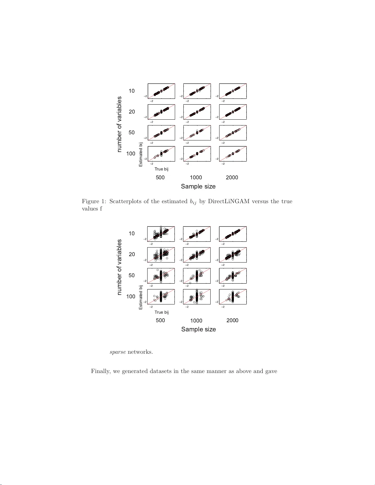
DirectLiNGAM: A direct metho d for learning a linear non-Gaussian structural equation mo del Shohei Shimizu ∗ , T ak a nori Inazumi † , Y asuhiro Soga w a ‡ , Aap o Hyv¨ arinen § , Y oshinobu Kaw ahara ¶ , T ak ashi W ashio k P atrik O. Ho y er ∗∗ , Kenneth Bollen †† , Abstract Structural equation models and Bay esian net w orks ha ve b een widely used to analyze causal relations b etw een conti nuous v ari ables. In such framew orks, linear acyclic models are typically used to mo del th e data- generating process of v ariables. Recently , it was sho wn that u se of n on - Gaussianit y iden tifies the full structu re of a linear acyclic mo del, i .e. , a causal ordering of v ariables a nd their connection strengths, without u sing any prior knowledge on th e netw ork structure, which is not the case with conv en tional metho d s. How ev er, existing estimation metho ds are based on iterativ e searc h algorithms and ma y not conv erge to a correct solution in a fi nite num b er of steps. In t h is pap er, we prop ose a new direct method to estimate a causal ordering and connection strengths based on non- Gaussianit y . In contras t to the previous metho ds, our algorithm requires no algorithmic parameters and is guaran teed to converge to the righ t solution within a smal l fix ed num b er of steps if the data strictly foll ow s the mo del. ∗ The Institute of Scientific and Industrial Research (ISIR), Osak a Univ ersit y , Mihogaok a 8-1, Ibaraki, Osak a 567-0047, Japan. Email: sshimi zu@ar.sank en.osak a-u.ac.jp † The Institute of Scientific and Industrial Research (ISIR), Osak a Univ er s it y , Mihogaok a 8-1, Ibaraki, Osak a 567-0047, Japan. Email: inazumi@ar.sanken.osak a-u.ac.j p ‡ The Institute of Scientific and Industrial Research (ISIR), Osak a Univ er s it y , Mihogaok a 8-1, Ibaraki, Osak a 567-0047, Japan. Email: sogaw a@ar.sanken.osak a-u.ac.j p § Departmen t of Computer Science, Department of Mathematics and Statistics and Helsi nki Institute for Information T echn ology , Uni versity of Helsinki, FIN-00014, Finland. Email: aapo.hyv ar inen@helsinki.fi ¶ The Institute of Scientific and Industrial Research (ISIR), Osak a Univ er s it y , Mihogaok a 8-1, Ibaraki, Osak a 567-0047, Japan. Email: k aw ahara@ar.sank en.osak a-u.ac.jp k The Institute of Scientific and Industrial Research (ISIR), Osak a Univ er s it y , Mihogaok a 8-1, Ibaraki, Osak a 567-0047, Japan. Email: washio@ar.sank en.osak a-u.ac.jp ∗∗ Departmen t of Computer Science, University of Helsi nki, FIN-00014, Finland. Email: patrik.ho ye r@helsinki.fi †† Departmen t of So ciology , CB 3210 H amilton Hall, Universit y of North Car olina, Chap el Hill, NC 27599-3210, U.S.A . Email: b ollen@unc.edu 1 1 In tro duction Many empirical sciences aim to discover and unders tand causal mechanisms underlying v a rious natura l phenomena and h uman so cial b ehavior. A n effec- tive wa y to study ca usal relationships is to conduct a co n trolled exper imen t. How ever, p erforming controlled exp eriments is often ethically imp ossible or to o exp ensive in many fields including so cial science s [1], bioinformatics [2] and neuroinformatics [3]. Thu s, it is necessary and imp orta nt to develop metho ds for causal inference based on the data that do not come from such co n trolled exp eriment s. Structural eq uation mo dels (SEM) [1] and Bay esian netw o rks (BN) [4, 5] ar e widely applied to ana lyze caus al rela tionships in many empirical studies. A line ar acyclic mo del that is a sp ecial case of SEM and BN is typically used to analyze ca usal effects b etw e en contin uo us v ariables . Estimation of the model commonly uses only the cov ar iance structure of the data and in mo s t case s can- not iden tify the full structure, i .e. , a causa l order ing and co nnection s trengths, of the model with no prior k no wledge on the structure [4, 5]. In [6], a non-Gaussia n v a r iant of SEM and BN calle d a linear no n-Gaussian acyclic model (LiNGAM) was prop osed, a nd its full str ucture was shown to be ident ifiable without pr e-sp ecifying a causal order of the v aria bles. This fea ture is a significa n t a dv antage ov er the con ven tional metho ds [4, 5]. A non- Ga ussian metho d to estimate the new mo del w as also developed in [6] and is clo sely re- lated to indep endent c o mponent a nalysis (ICA) [7]. In the subsequen t studies , the no n-Gaussian framework has b een ex tended in v a rious dir ections for learn- ing a wider v a riety of SEM and BN [8 – 10]. In what follows, we r efer to the non-Gaussian mo del a s LiNGAM and the estimation metho d as IC A- L iNGAM algorithm. Most of ma jo r ICA algorithms including [11, 12] are iterative s earch metho ds [7]. Therefore, the ICA-LiNGAM a lgorithms based on the ICA algorithms need some additiona l infor mation including initial guess and co nvergence criter ia. Gradient-based methods [11] further need step sizes. How e ver, such a lgorithmic parameters are hard to optimize in a systematic w ay . Th us, the ICA-bas e d algorithms may get stuck in lo cal optima and may not c o n verge to a reaso nable solution if the initia l guess is badly chosen [1 3]. In this pap er, we prop ose a new dire ct metho d to estimate a causal o rdering of v aria bles in the LiNGAM without prior k nowledge on the str ucture. The new metho d estimates a c a usal order of v a riables by successively reducing eac h independent comp onent fro m given data in the model, and this proc e ss is com- pleted in steps equa l to the num b er of the v ar iables in the mo del. It is no t based on iterativ e search in the p ar ameter sp ac e a nd needs no initial guess o r similar algorithmic parameters. It is guar ant e e d to conv er g e to the right so lution w ithin a small fixed n umber of steps if the data st rictly follo ws the model, i.e. , if a ll the mo del assumptions are met and the sample size is infinite. These features of the new method enable more accurate estimatio n of a causal o r der of the v aria bles in a disambiguated a nd direct pro cedure. Once the caus a l or ders of v a riables is ident ified, the co nnection streng ths betw een the v ariable s are e asily estimated 2 using some con ven tiona l cov aria nce-based metho ds s uc h as leas t squares and maximum likeliho o d appro a c hes [1]. W e also sho w ho w prio r knowledge on the structure can be incorp orated in the new metho d. The pap er is structured as follows. First, in Section 2, w e briefly r eview LiNGAM and the ICA-based LiNGAM a lgorithm. W e then in Section 3 in tro- duce a new dir ect method. The p erformance of the new method is examined by exp eriments on ar tificial data in Section 4, and exp eriments on real-world data in Section 5. Conclusions are given in Section 6. P reliminary r e sults were presented in [1 4–16]. 2 Bac kground 2.1 A linear non-Gaussian acyclic mo del: LiNGAM In [6], a non-Gauss ian v ar ian t of SEM and BN, which is called LiNGAM, w as prop osed. Assume that obs erved da ta are generated from a pro cess re presented graphically by a direc ted acyclic gr aph, i.e. , D AG. Let us represent this DA G by a m × m adjacency matrix B = { b ij } where every b ij represents the c o nnection strength from a v a riable x j to another x i in the DA G. Moreover, let us denote by k ( i ) a causa l o rder of v a riables x i in the DA G so that no la ter v aria ble determines or has a dir ected path on an y ear lier v aria ble . (A directed path from x i to x j is a sequence of directed edges such that x j is reachable from x i .) W e further assume that the relations b etw ee n v ariables a re linear. Without loss of g enerality , each obs erved v ar iable x i is assumed to hav e zero mean. Then we hav e x i = X k ( j ) 0 is the bandwidth of Gaussia n kernel. F urther let κ denote a small po sitiv e co nstan t. Then, in [22], the kernel-based estimator of mut ual informa- tion is defined a s: d M I ker nel ( y 1 , y 2 ) = − 1 2 log det K κ det D κ , (11) where K κ = "  K 1 + nκ 2 I  2 K 1 K 2 K 2 K 1  K 2 + nκ 2 I  2 # (12) D κ = "  K 1 + nκ 2 I  2 0 0  K 2 + nκ 2 I  2 # . (13) As the bandwidth σ of Gaus s ian kernel tends to ze r o, the p opulation co un terpart of the estimato r converges to the mutual information up to second order when it is expanded aro und distributions with tw o v aria bles y 1 and y 2 being independent [22]. The determinants of the Gr am matrices K 1 and K 2 can be efficiently 2 Matlab codes can b e do wnloaded at http: //www.di. ens.fr/ ~ fbach/ke rnel- ica/index.htm 9 computed by using the incomplete Cho lesky decomp osition to find their low- rank a pproximations of rank M ( ≪ n ). In [22], it was suggested that the p ositive constant κ and the width o f the Gaussian kernel σ are set to κ = 2 × 10 − 3 , σ = 1 / 2 for n > 1000 and κ = 2 × 1 0 − 2 , σ = 1 for n ≤ 1000 due to so me theoretical and computational considerations. In this pap er, we use the kernel-based independence mea sure. W e first ev al- uate pa ir wise indep endence b etw een a v ariable a nd ea c h of the residuals and next take the sum of the pairwise mea sures ov er the residua ls. Let us denote b y U the set of the subscripts of v a r iables x i , i.e. , U = { 1, · · · , p } . W e use the fol- lowing statistic to ev aluate indepe ndence b et ween a v ariable x j and its residuals r ( j ) i = x i − cov( x i ,x j ) v ar( x j ) x j when x i is regressed on x j : T ker nel ( x j ; U ) = X i ∈ U,i 6 = j d M I ker nel ( x j , r ( j ) i ) . (14) Many other nonparametric independence measures [23 , 24] and mo re computa- tionally simple measure s that use a sing le no nlinear correlatio n [25] hav e als o bee n pro pos ed. An y such prop osed metho d o f indepe ndenc e co uld p o ten tially be used instea d of the kernel-based measur e in E q. (14). 3.2 DirectLiNGAM algorithm W e no w prop ose a new direc t alg orithm called DirectLiNGAM to estimate a causal or dering and the connec tio n strengths in the LiNGAM (2): DirectLiNGAM alg or ithm 1. Given a p -dimensional rando m vector x , a set of its variable subscripts U and a p × n da ta matrix of the random vector as X , i n itialize an o rdered list of va riables K := ∅ and m := 1 . 2. Rep eat until p − 1 subscripts are app ended to K : (a) Perfo rm lea s t squares regressions of x i on x j for all i ∈ U \ K ( i 6 = j ) and compute the residual vector s r ( j ) and the residual data matrix R ( j ) from the d a ta matrix X for all j ∈ U \ K . Find a var iable x m that is most i ndepe n dent of its residuals : x m = arg min j ∈ U \ K T ker nel ( x j ; U \ K ) , (15) where T ker nel is the indep endence measure defined in Eq. (14). (b) App end m to the end o f K . (c) Let x := r ( m ) , X := R ( m ) . 3. App end the remaining va riable to th e end of K . 10 4. Construct a strictly lower triangular matrix B by following th e order in K , and estimate the connectio n strengths b ij by using some co nventional covariance- based regression s uch as least s qua res and maximum likeliho o d ap proaches on the original random vector x and the or iginal data matrix X . We use leas t squares regression in this pa p er. 3.3 Computational complexit y Here, we consider the computational complexity o f DirectLiNGAM compar ed with the ICA-LiNGAM with resp ect to sample size n and n umber of v aria bles p . A dominant part of DirectLiNGAM is to co mpute Eq. (14) for each x j in Step 2(a). Since it requires O ( np 2 M 2 + p 3 M 3 ) op erations [22] in p − 1 iterations, complexity of the step is O ( np 3 M 2 + p 4 M 3 ), where M ( ≪ n ) is the maximal rank found b y the low-rank decompo sition used in the kernel-based indep endence measure. Another dominant part is the regressio n to e stimate the matrix B in Step 4. The complexity of many represe ntative r e g ressions including the least square algor ithm is O ( np 3 ). Hence, we hav e a total budget of O ( np 3 M 2 + p 4 M 3 ). Meanwhile, the ICA-LiNGAM r equires O ( p 4 ) time to find a ca usal order in Step 5. Complexity of a n iteration in F as tICA pro cedure at Step 1 is k no wn to b e O ( np 2 ). Assuming a constant num b er C o f the iterations in F a stICA steps, the complexity of the ICA-LiNGAM is consider ed to be O ( C np 2 + p 4 ). Though genera l ev a luation of the r equired iteration num b er C is difficult, it can be conjectured to grow linearly with regards to p . Hence the co mplexit y of the ICA-LiNGAM is presumed t o be O ( np 3 + p 4 ). Thu s, the computationa l co s t of DirectLiNGAM w o uld b e large r than that of IC A- L iNGAM esp e cially when the low-rank approximation of the Gram ma- trices is not so efficien t, i.e. , M is lar ge. Ho wever, we note the fact that Di- rectLiNGAM has guaranteed con vergence in a fixed num ber of s teps and is of known complexit y , whereas for typical ICA algorithms including F as tICA, the run-time co mplexit y and the very convergence ar e not guarant eed. 3.4 Use of prior kno wledge Although DirectLiNGAM requires no prio r knowledge on the structure, more efficient learning can be achieved if some pr ior knowledge on a par t o f the structure is av ailable b ecause then the n umber of ca usal orders and connection strengths to be estimated gets smaller. W e present thre e lemmas to utilize prior knowledge in DirectLiNGAM. Let us first define a ma tr ix A knw =[ a knw j i ] that collects prior k no wledge under the LiNGAM (2) as follows: a knw j i :=        0 if x i do es not hav e a directed path to x j 1 if x i has a directed path to x j − 1 if no pr io r knowledge is a v ailable to kno w if either of the t w o cases above (0 or 1) is true . (16) 11 Due to the definition o f exogeno us v ariables and that of prio r knowledge matrix A knw , w e readily obtain the following three lemmas. Lemma 3 Assume that the i nput data x strictly fo l lows the LiNGAM (2). An observe d variable x j is exo genous if a knw j i is zer o for al l i 6 = j . Lemma 4 Assume that the i nput data x strictly fo l lows the LiNGAM (2). An observe d variable x j is endo genous, i.e., not exo genous, if ther e exist such i 6 = j that a knw j i is unity. Lemma 5 Assume that the i nput data x strictly fo l lows the LiNGAM (2). An observe d variable x j do es not r e c eive the effe ct of x i if a knw j i is zer o. The principle of making DirectLiNGAM algorithm more a ccurate and faster based on prior kno wledge is as follows. W e first find an exog enous v aria ble by applying Lemma 3 instead of Lemma 1 if an exo genous v ariable is identi- fied based o n prior knowledge. Then w e do no t ha ve to ev aluate indepe ndence betw een a n y obser ved v ariable a nd its residuals. If no exog enous v ariable is ident ified based on prior knowledge, we next find endogenous (non-exogenous) v ariables by applying Lemma 4. Since endogeno us v ar iables are never exo g enous we can narrow down the search space to find an ex o genous v a r iable bas ed on Lemma 1. W e can further skip to compute the residual o f an observ ed v a riable and take the v a riable itself as the residual if its r egressor do es no t rec eiv e the effect of the v a riable due to L emma 5. Th us, we can decrease the num b er of causal order s and connection strengths to be estimated, and it improves the accuracy and computational time. The pr inciple can a lso be used to further an- alyze the r esiduals and find the next exog enous res idual b ecause of Corollary 1. T o implement these ideas, we only hav e to repla ce Step 2a in DirectLiNGAM algorithm by the follo wing s teps: 2a-1 Find such a variable(s) x j ( j ∈ U \ K ) that the j -th row of A knw has zero in the i -th column for all i ∈ U \ K ( i 6 = j ) and denote the set o f such va riab l es by U exo . If U exo is no t empty , set U c := U exo . If U exo is empty , find such a var iable(s) x j ( j ∈ U \ K ) that the j - th ro w of A knw has unity in the i -th column fo r at least one o f i ∈ U \ K ( i 6 = j ), denote the set of such variables by U end and set U c := U \ K \ U end . 2a-2 Denote b y V ( j ) a set of such a variable subscript i ∈ U \ K ( i 6 = j ) that a knw ij = 0 fo r all j ∈ U c . First s et r ( j ) i := x i for all i ∈ V ( j ) , next perform least squares regressions of x i on x j for all i ∈ U \ K \ V ( j ) ( i 6 = j ) and estimate the residual vectors r ( j ) and the r esidual data matrix R ( j ) from the data matrix X for al l j ∈ U c . If U c has a single va riable, set the variable to b e x m . Otherwis e, find a variable x m in U c that is most independent of the residuals: x m = arg min j ∈ U c T ker nel ( x j ; U \ K ) , (17) where T ker nel is the indep endence measure defined in Eq. (14). 12 4 Sim ulations W e first randomly gener ated 5 datasets base d on spar se net works under each combination of n umber of v ariables p and s a mple size n ( p =10, 20, 50 , 10 0; n =500 , 10 00, 2000 ): 1. W e constr ucted the p × p adjacency matrix with all z e ros and replace d every element in the lo w er-tria ngular part b y independent realizations of Bernoulli random v a riables with succe s s pro ba bilit y s similar ly to [26]. The probability s determines the sparseness of the mo del. The exp ected nu mber of adjacent v a riables of ea c h v a riable is g iven b y s ( p − 1). W e randomly set the spars eness s so that the n umber of adjac e n t v ar iables was 2 o r 5 [26]. 2. W e repla ced each non-zer o (unit y) entry in the adjacency matr ix by a v alue randomly chosen from the in terv al [ − 1 . 5 , − 0 . 5 ] ∪ [0 . 5 , 1 . 5] a nd selected v ariances of the exter nal influences e i from the interv a l [1 , 3 ] as in [27]. W e used the r e s ulting matrix as the data-g enerating a djacency ma trix B . 3. W e g enerated data with sample size n by indep endently drawing the ex- ternal influence v a riables e i from v ar ious 18 no n- Gaussian distributions used in [22] including (a) Student with 3 degr ees of free do m; (b) double exp onent ial; (c) uniform; (d) Studen t with 5 deg rees of freedom; (e) ex- po nen tial; (f ) mixture of tw o double exp onentials; (g)-(h)-(i) symmetric mixtures of tw o Gaussians: m ultimo dal, transitional and unimo dal; (j)- (k)-(l) nons ymmetric mixtures of tw o Ga ussians, multimodal, trans itio nal and unimoda l; (m)-(n)-(o) symmetric mixtures of four Gaussians: multi- mo dal, trans itional and unimo dal; (p)-(q)-(r) nonsymmetric mixtures of four Gaussians: multimodal, trans itional a nd unimo dal. See Fig . 5 of [22] for the shap es of the pro babilit y density functions. 4. The v alue s o f the observed v ar iables x i were generated according to the LiNGAM (2 ). Finally , we r andomly p ermuted the order of x i . F urther we similarly g enerated 5 data s ets based o n dense (full) net works, i.e. , full D A Gs with every pair of v a riables is co nnec ted by a directed edge, under each combination of num b er o f v ariables p and sample s ize n . Then we tested Di- rectLiNGAM and ICA-LiNGAM on the da tasets ge nerated by spars e net works or dense (full) net works. F or ICA-LiNGAM, the maximum num be r of iterations was taken as 1000 [6]. The exp eriments were conducted on a standa rd PC using Matlab 7 .9. Matlab implemen tations of the tw o metho ds are av aila ble on the web: DirectLiNGAM: ht tp://ww w.ar.sank en.osaka- u.ac.jp/ ~ inazum i/dlin gam.html ICA-LiNGAM: h ttp://w ww.cs.h elsinki.fi/group/neuroinf/lingam/ . W e computed the distance b etw een the true B and ones estimated by Di- rectLiNGAM and ICA-LiNGAM using the F robenius norm defined as q trace { ( B tr ue − b B ) T ( B tr ue − b B ) } . (18) 13 T able 1: Median distances (F robenius nor ms) betw een true B and es timated B of DirectLiNGAM and ICA-LiNGAM with fiv e replications. Sp arse net works Sample size 500 1000 2000 DirectLiNGAM dim. = 10 0.48 0.31 0.21 dim. = 20 1.19 0.70 0.50 dim. = 50 2.57 1.82 1.40 dim. = 100 5.75 4.61 2.35 ICA-LiNGAM dim. = 10 3.01 0.74 0.65 dim. = 20 9.68 3.00 2.06 dim. = 50 20.61 20.23 12.91 dim. = 100 40.77 43.74 36.52 DirectLiNGAM with dim. = 10 0.48 0.30 0.24 prior knowledge (50%) dim. = 20 1.00 0.71 0.49 dim. = 50 2.47 1.75 1.1 9 dim. = 100 4.9 4 3.89 2.27 Dense (full) net works Sample size 500 1000 2000 DirectLiNGAM dim. = 10 0.45 0.46 0.2 0 dim. = 20 1.46 1.53 1.1 2 dim. = 50 4.40 4.57 3.8 6 dim. = 100 7.38 6.81 6.1 9 ICA-LiNGAM dim. = 10 1.71 2.08 0.3 9 dim. = 20 6.70 3.38 1.8 8 dim. = 50 17.28 16.66 12.05 dim. = 100 34.95 34.02 32.02 DirectLiNGAM with dim. = 10 0.45 0.31 0.1 9 prior knowledge (50%) dim. = 20 0.8 4 0.90 0.41 dim. = 50 2.48 1.86 1.5 6 dim. = 100 4.6 7 3.60 2.61 T ables 1 and 2 s ho w the media n distances (F rob enius nor ms) and median compu- tational times (CP U times) resp ectively . In T able 1, DirectLiNGAM was b etter in distances of B and ga ve more accurate estimates of B tha n ICA-LiNGAM for all of the conditions. In T a ble 2 , the computation amount o f Dir ectLiNGAM was rather larg er than ICA-LiNGAM when the sample size was increased. A main bottleneck of computation was the kernel-based independence mea sure. How ever, its computation amo unt c a n b e considere d to b e still tracta ble. In fact, the a ctual elapsed times were approximately one- q uarter of their CPU times res pectively probably b ecause the CPU had four cor e s. Interestingly , the CPU time of ICA-LiNGAM actua lly dec reased with increased sa mple size in 14 T able 2: Median computational times (CPU times) o f Direc tLiNGAM and ICA- LiNGAM with fiv e re plications. Sp arse net works Sample size 500 1000 2000 DirectLiNGAM dim. = 1 0 15.16 sec. 37 .21 sec. 66 .75 sec. dim. = 2 0 1.56 min. 5.75 min. 17.22 mi n. dim. = 5 0 16 .25 min. 1.34 hr s . 2.70 hrs. dim. = 100 2.35 hrs. 21 .17 hrs. 19.90 hrs. ICA-LiNGAM dim. = 1 0 0.73 sec . 0.41 s e c. 0.28 s ec. dim. = 2 0 5.40 sec . 2.45 s e c. 1.14 s ec. dim. = 5 0 14.49 sec. 21 .47 sec. 32 .03 sec. dim. = 100 46 .32 sec. 58.02 s ec. 1 .16 min. DirectLiNGAM with dim. = 10 4.13 sec. 17.75 sec. 30 .9 5 sec. prior kno wledge (50%) dim. = 20 28.02 sec. 1.64 min. 4.98 min . dim. = 5 0 7.62 min. 28 .89 min. 1.09 hr s. dim. = 100 48.28 min. 1.84 hrs. 7.51 hrs . Dense (full) net works Sample size 500 1000 2000 DirectLiNGAM dim. = 1 0 8.05 sec . 24.52 sec. 4 9.44 sec. dim. = 2 0 1.00 min. 4.23 min. 6.91 min. dim. = 5 0 16 .18 min. 1.12 hr s . 1.92 hrs. dim. = 100 2.16 hrs. 8.59 hr s . 17 .24 hrs. ICA-LiNGAM dim. = 1 0 0.97 sec . 0.34 s e c. 0.27 s ec. dim. = 2 0 5.35 sec . 1.25 s e c. 4.07 s ec. dim. = 5 0 15.58 sec. 21 .01 sec. 31 .57 sec. dim. = 100 47 .60 sec. 56.57 s ec. 1 .36 min. DirectLiNGAM with dim. = 10 2.67 sec. 5.66 sec. 1 2 .31 sec. prior kno wledge (50%) dim. = 20 5.02 sec. 31.7 0 sec. 38.3 5 sec. dim. = 5 0 46.74 sec. 2.89 min. 5.0 0 min. dim. = 100 3.19 min. 10.44 min. 19.80 min. some ca ses. This is presumably due to better con vergence pr ope r ties. T o visua lize the estimation results, Figure s 1, 2, 3 and 4 give com bined scat- terplots of the estimated elements of B of DirectLiNGAM and ICA-LiNGAM versus the true ones for s parse netw o rks and dense (full) netw o rks resp ectively . The differen t plots corresp ond to different n um be r s of v ar iables and different sample sizes, where each plo t c o m bines the data for differen t adjacency matri- ces B and 18 differen t distributions of the ex ter nal influences p ( e i ). W e can see that DirectLiNGAM worked well a nd better than ICA-LiNGAM, as evidenced by the grouping o f the data p oints onto the ma in diag onal. 15 0 2 0 2 0 2 0 2 0 2 0 2 0 2 0 2 0 2 0 2 0 2 0 2 0 2 0 2 0 2 0 2 0 2 0 2 0 2 0 2 0 2 0 2 0 2 0 2 T rue bij Estimated bij 500 1000 2000 Sample size number of variables 10 20 50 100 Figure 1: Scatterplots of the es timated b ij by DirectLiNGAM v ersus the true v alues f or sp arse net works. 0 2 0 2 0 2 0 2 0 2 0 2 0 2 0 2 0 2 0 2 0 2 0 2 0 2 0 2 0 2 0 2 0 2 0 2 0 2 0 2 0 2 0 2 0 2 0 2 T rue bij Estimated bij 500 1000 2000 Sample size number of variables 10 20 50 100 Figure 2: Scatterplots of the estimated b ij by ICA-LiNGAM versus the true v alues f or sp arse net works. Finally , w e generated da tasets in the same manner as ab ov e and gave so me prior knowledge to DirectLiNGAM by crea ting prior knowledge matrices A knw as follo ws. W e first replaced ev ery non-z ero e le men t b y unit y and every diag o nal element by ze ro in A =( I − B ) − 1 and subsequently hid each of the off-dia gonal elements, i.e. , r eplaced it b y − 1, with pro babilit y 0 . 5. The b o ttoms of T ables 1 and 2 sho w the median distances and media n computational times. It was em- 16 0 2 0 2 0 2 0 2 0 2 0 2 0 2 0 2 0 2 0 2 0 2 0 2 0 2 0 2 0 2 0 2 0 2 0 2 0 2 0 2 0 2 0 2 0 2 0 2 T rue bij Estimated bij 500 1000 2000 Sample size number of variables 10 20 50 100 Figure 3: Scatterplots of the es timated b ij by DirectLiNGAM v ersus the true v alues f or dense (full) net works. 0 2 0 2 0 2 0 2 0 2 0 2 0 2 0 2 0 2 0 2 0 2 0 2 0 2 0 2 0 2 0 2 0 2 0 2 0 2 0 2 0 2 0 2 0 2 0 2 T rue bij Estimated bij 500 1000 2000 Sample size number of variables 10 20 50 100 Figure 4: Scatterplots of the estimated b ij by ICA-LiNGAM versus the true v alues f or dense (full) net works. pirically confirmed tha t use of prior knowledge gav e mor e accur ate estimates and less computatio nal times in most ca ses es pecia lly for dense (f ull) net works. The reaso n would probably b e that for dense (full) netw orks more pr ior knowl- edge ab out where dir ected paths exist were likely to b e given and it narrowed down the sea rch space more efficiently . 17 1 2 Figure 5: Abstr act mo del of the double-pendulum used in [29]. 5 Applications to real-w orld data W e here apply DirectLiNGAM and ICA-LiNGAM on real-world physics and so ciology data. Both DirectLiNGAM and ICA-LiNGAM estimate a ca usal or- dering of v ar ia bles and pr ovide a full DA G. Then we hav e tw o options to do further analysis [9]: i) Find significant directed edg es or direct ca usal effects b ij and s ig nificant total causal effects a ij with A =( I − B ) − 1 ; ii) Estimate redundant directed edg es to find the underlying D AG. W e demonstrate an exa mple of the former in Subsection 5.1 and that of the latter in Subsection 5 .2. 5.1 Application t o ph ysical data W e applied DirectLiNGAM and ICA-LiNGAM on a dataset crea ted from a ph ysical sys tem called a double-p endulum, a p endulum with another p endulum attached to its end [2 8] as in Fig. 5. The dataset was first used in [29]. T he raw data consisted o f four time series pr ovided b y Ibaraki University (Japan) filming the pendulum system with a high-spe ed video ca mer a at every 0.01 second for 20.3 s econds a nd then reading out the p osition using an image analysis s o ft w are. The fo ur v a riables were θ 1 : the angle betw een the top limb and the vertical, θ 2 : the angle b et ween the b ottom limb and the vertical, ω 1 : the angula r sp eed of θ 1 or ˙ θ 1 and ω 2 : the angular sp eed of θ 2 or ˙ θ 2 . The n umber of time points was 2035. The dataset is a v ailable on the w eb: http:/ /www.a r.sanken.osaka- u.ac.jp/ ~ inazum i/data /furiko.html In [29], some theo retical considera tions based on the do main knowledge im- plied that the angle sp e eds ω 1 and ω 2 are mainly determined by the angles θ 1 and θ 2 in both ca ses where the swing of the pendulum is sufficiently sma ll ( θ 1 , θ 2 ≈ 0) and where the swing is not very small. F urther, in practice, it was reasona ble to assume tha t there w e re no laten t confounders [2 9]. As a pre pr o cessing, we firs t remov e d the time dep endency from the raw data using the ARMA (AutoRegres sive Moving Average) mo del with 2 autore- gressive terms and 5 mo ving av era ge terms following [29]. Then we applied DirectLiNGAM a nd ICA-L iNGAM on the prepro cessed da ta. The estimated 18 Æ 1 Æ 2 Ö 1 Ö 2 Æ 1 Æ 2 Ö 1 Ö 2 DirectLiNGAM ICA-LiNGAM Figure 6: Left: The estima ted netw or k by DirectLiNGAM. Only s ignificant directed edges ar e shown with 5 % significanc e level. Right: The estimated net work by ICA-LiNGAM. No significa n t directed edges w ere found with 5% significance level. Æ 1 Æ 2 Ö 1 Ö 2 PC GES Æ 1 Æ 2 Ö 1 Ö 2 Figure 7: Left: The estimated net work b y PC alg orithm with 5% s ig nificance level. Rig h t: The estimated net work b y GES. An undirected edge b et ween t w o v ariables mea ns that there is a directed edge fro m a v ariable to the other or the reverse. adjacency matrices B o f θ 1 , θ 2 , ω 1 and ω 2 were as fo llows: DirectLiNGAM :     θ 1 θ 2 ω 1 ω 2 θ 1 0 0 0 0 θ 2 − 0 . 23 0 0 0 ω 1 90 . 39 − 2 . 88 0 0 ω 2 5 . 65 94 . 64 − 0 . 1 1 0     , (19) ICA − LiNGAM :     θ 1 θ 2 ω 1 ω 2 θ 1 0 0 0 0 θ 2 1 . 45 0 0 0 ω 1 108 . 82 − 52 . 73 0 0 ω 2 216 . 26 112 . 5 0 − 1 . 89 0     . (20) The estimated orderings b y DirectLiNGAM and ICA-LiNGAM w ere iden tica l, 19 but the estimated connection strengths were very different. W e further com- puted their 95% confidence in terv als b y using bo otstra pping [30] with the num- ber of b oo tstrap replicates 100 00. T he estimated netw o rks b y Dir ectLiNGAM and ICA-LiNGAM a r e g raphically shown in Fig. 6, where o nly significant di- rected edges (direct causal effects) b ij are shown with 5% significance level. 3 DirectLiNGAM found tha t the a ngle sp eeds ω 1 and ω 2 were deter mined by the angles θ 1 or θ 2 , whic h was consisten t with the domain kno wledge. Tho ug h the directed edg e from θ 1 to θ 2 might b e a bit difficult to in ter pret, the effect of θ 1 on θ 2 was e s timated to b e neg ligible since the co efficien t of deter mination [1] of θ 2 , i.e. , 1 − v ar( ˆ e 2 )/v ar( ˆ θ 2 ), was very small and w a s 0.01. (The coefficient of determination of ω 1 and that of ω 2 were 0 .46 and 0.49 re spectively .) On the other hand, ICA-LiNGAM could no t find a n y significant direc ted e dg es s ince it gav e very differen t estimates for differ e n t b o otstrap samples. F or further comparison, we also tested tw o co n ven tional methods [31, 32] based on co nditional indep endences. Fig. 7 shows the estimated netw orks by PC algor ithm [31] with 5% significance level and GE S [32] with the Gaussia nit y assumption. W e used the T e trad IV 4 to run the t wo methods. PC algo rithm found the same dir ected edge fro m θ 1 on ω 1 as DirectLiNGAM did but did not found the directed edge from θ 2 on ω 2 . GES found the same directed edge from θ 1 on θ 2 as DirectLiNGAM did but did no t find that the angle spe eds ω 1 and ω 2 were determined b y the angles θ 1 or θ 2 . W e also c o mputed the 95% confidence interv a ls of the total causa l effects a ij using b o otstrap. DirectLiNGAM found s ignificant total causa l effects fr o m θ 1 on θ 2 , from θ 1 on ω 1 , from θ 1 on ω 2 , from θ 2 on ω 1 , and fro m θ 2 on ω 2 . These significant total effects would also b e reas o nable based on similar arg umen ts. ICA-LiNGAM o nly found a significant total causal effect from θ 2 on ω 2 . Overall, although the four v ariables θ 1 , θ 2 , ω 1 and ω 2 are likely to be nonlin- early related according to the domain kno wle dge [28, 2 9], DirectLiNGAM gav e int eresting results in this example. 5.2 Application t o so ciology data W e analyzed a dataset taken fro m a s oc io logical data repo sitory on the Inter- net called General So cial Survey ( http ://www. norc.org/GSS+Website/ ). The data consisted o f six obser ved v ariables, x 1 : father’s o ccupation le vel, x 2 : so n’s income, x 3 : father’s education, x 4 : s on’s oc cupation level, x 5 : son’s educa- tion, x 6 : num b er of siblings. The sample selection was conducted based on the following criteria: i) non-farm ba c kground (ba s ed o n tw o measures of father’s o ccupation); ii) ages 35 to 44; iii) white; iv) male; v) in the lab or force at the time of the s urvey; vi) not mis s ing data for any of the cov ariates ; vii) years 1972- 2006. The sa mple size was 13 80. Fig. 8 shows domain knowledge ab out their ca usal relations [3 3]. As shown in the figure, there could b e so me latent confounders betw een x 1 and x 3 , x 1 and x 6 , or x 3 and x 6 . An ob jective o f this 3 The issue of multiple comparisons arises in this con text, which w e would lik e to study in future work. 4 http://w ww.phil.cm u.edu/projects/tetrad/ 20 Fathe r Õ s Education (x3) Fathe r Õ s Occupatio n (x1) Son Õ s Education (x5) Number of Siblings (x6) Son Õ s Occupatio n (x4) Son Õ s Income (x2) Figure 8: Sta tus attainment mo del based on domain knowledge [33]. A bi- directed edge b etw e en t wo v ariables means that the r elation is not mo deled. F or instance, there could b e la ten t co nfo unders betw een the tw o, there could b e a dir e c ted edge betw een the t wo, or the tw o could be independent. example was to see how our metho d b ehav es when such a model assumption of LiNGAM co uld b e violated that th ere is no laten t confounder . The estimated a djacency ma trices B by DirectLiNGAM a nd I CA- LiNGAM were a s follows: DirectLiNGAM :         x 1 x 2 x 3 x 4 x 5 x 6 x 1 0 0 3 . 19 0 . 10 0 . 41 0 . 21 x 2 33 . 48 0 4 52 . 84 422 . 87 1 645 . 45 347 . 96 x 3 0 0 0 0 0 . 55 − 0 . 1 8 x 4 0 0 0 . 17 0 4 . 61 − 0 . 19 x 5 0 0 0 0 0 − 0 . 12 x 6 0 0 0 0 0 0         , (21) ICA − LiNGAM :         x 1 x 2 x 3 x 4 x 5 x 6 x 1 0 0 0 . 93 0 − 0 . 68 − 0 . 20 x 2 50 . 70 0 − 31 . 82 200 . 84 65 . 63 336 . 04 x 3 0 0 0 0 0 . 24 − 0 . 2 7 x 4 0 . 17 0 − 0 . 40 0 − 0 . 14 − 0 . 14 x 5 0 0 0 0 0 0 x 6 0 0 0 0 − 0 . 08 0         . ( 22) W e subsequent ly pr uned re dundan t directed edges b ij in the full D AGs b y rep eatedly a pplying a sparse method called Adaptiv e Las so [34] on ea c h v a riable and its p otential pa rent s. See Appendix A for some more details of Ada ptive Lasso. W e used a matlab implemen tation in [35] to run the La sso. Then we 21 obtained the following pruned a dja c ency matrices B : DirectLiNGAM :         x 1 x 2 x 3 x 4 x 5 x 6 x 1 0 0 3 . 1 9 0 0 0 x 2 0 0 0 4 22 . 87 0 0 x 3 0 0 0 0 0 . 55 0 x 4 0 0 0 0 4 . 61 0 x 5 0 0 0 0 0 − 0 . 12 x 6 0 0 0 0 0 0         , (23) ICA − LiNGAM :         x 1 x 2 x 3 x 4 x 5 x 6 x 1 0 0 0 . 9 3 0 0 0 x 2 0 0 0 2 00 . 84 0 0 x 3 0 0 0 0 0 . 24 0 x 4 0 0 0 0 − 0 . 14 0 x 5 0 0 0 0 0 0 x 6 0 0 0 0 − 0 . 08 0         . (24) The estimated net works b y DirectLiNGAM a nd ICA-LiNGAM are graphi- cally shown in Fig. 9 a nd Fig. 1 0 resp ectively . All the direc ted edges estimated by DirectLiNGAM were r easonable to the domain k no wledge other than the directed e dg e from x 5 : son’s education to x 3 : father’s education. Since the sample size was la rge and yet the estima ted mo del was not fully cor rect, the mistake on the dire c ted edge b e t w een x 5 and x 3 might imply that so me mo del assumptions migh t b e more or less violated in the data. ICA-LiNGAM gave a similar estimated netw or k but did one mo r e mistak e that x 6 : n um be r of siblings is determined b y x 5 : so n’s education. F urther, Fig. 11 and Fig. 1 2 show the estimated netw orks b y PC alg orithm with 5% significa nce level and GE S with the Ga ussianity a ssumption. B oth of the conv entional metho ds did not find the directions of many edg e s . The t wo conv entional methods found a reasona ble direction of the edg e b etw een x 1 : father’s o ccupation and x 3 : father’s education, but they gav e a wrong dir ection of the edge b etw een x 1 : father’s occ upation and x 4 : so n’s o ccupation. 6 Conclusion W e presented a new es timation algorithm for the LiNGAM that ha s guara n teed conv er gence to the right s olution in a fixed num b er of steps if the data strictly follows the mo del and known computational complexity unlike most ICA meth- o ds. This is the first algor ithm spe c ia lized to estimate the LiNGAM. Simulations implied that the new metho d often provides better statistica l p e rformance than a sta te of the a rt metho d based o n ICA. In r eal-world applications to physics and so ciology , promising results were obtained. F uture w orks would include i) assessment of practical p erformance of statistical tests to detect viola tions of the mo del assumptions including tests o f indep endence [36]; ii) implementation issues of our alg orithm to impro ve the practical computational efficiency . 22 Fathe r Õ s Education (x3) Fathe r Õ s Occupatio n (x1) Son Õ s Education (x5) Number of Siblings (x6) Son Õ s Occupatio n (x4) Son Õ s Income (x2) Figure 9: The estimated net work b y Dir ectLiNGAM and Adaptive Lasso. A red so lid directed edge is reasonable to the domain kno wledge. Fathe r Õ s Education (x3) Fathe r Õ s Occupatio n (x1) Son Õ s Education (x5) Number of Siblings (x6) Son Õ s Occupatio n (x4) Son Õ s Income (x2) Figure 10: The estimated netw ork by ICA-LiNGAM and Adaptive Lasso. A red so lid directed edge is reasonable to the domain kno wledge. Ac kno wledgemen ts W e are very grateful to Hiros hi Haseg aw a (Colleg e of Scie nce, Ibar a ki University , Japan) for providing the ph ysics data and Satoshi Hara and Ayumu Y amaok a for int eresting discussio n. This work was par tially carried out at Department of Mathematical a nd Computing Sciences a nd Department of Computer Sci- ence, T okyo Institute of T e chnology , Japan. S.S., Y.K. and T.W. were partia lly suppo rted by ME XT Grant-in-Aid for Y oung Scientists #217003 02, by JSP S Grant-in-Aid for Y oung Scientists #2 080001 9 and by Grant-in-Aid for Scien- tific Res earch (A) #192000 13, resp ectively . S.S. and Y.K. were partially sup- po rted b y J SPS Global CO E program ‘Computationism as a F oundation for the Sciences’. A.H. was partially suppo rted b y the Academy of Finland Cen tre of Excellence for Algorithmic Data Analysis. 23 Fathe r Õ s Education (x3) Fathe r Õ s Occupatio n (x1) Son Õ s Education (x5) Number of Siblings (x6) Son Õ s Occupatio n (x4) Son Õ s Income (x2) Figure 11: The estimated netw ork b y PC alg orithm with 5% sig nificance lev el. An undirected edge b etw een tw o v a r iables means that there is a directed edge from a v ar iable to the other or the reverse. A r ed solid dir ected edge is reaso nable to the domain knowledge. Fathe r Õ s Education (x3) Fathe r Õ s Occupatio n (x1) Son Õ s Education (x5) Number of Siblings (x6) Son Õ s Occupatio n (x4) Son Õ s Income (x2) Figure 12 : The estimated netw o rk b y GE S. An undire cted edge b etw een tw o v ariables mea ns that there is a directed edge fro m a v ariable to the other or the reverse. A red solid directed edge is reasonable to the domain kno wledge. A Adaptiv e Lasso W e v ery briefly review the adaptive Lasso [34], which is a v aria n t of the Lasso [37]. See [34] for more details. The adaptiv e Las so is a reg ularization technique for v a riable selectio n and assumes the same data g enerating pr oce ss as LiNGAM: x i = X k ( j )