The algebraic difference of two random Cantor sets: The Larsson family

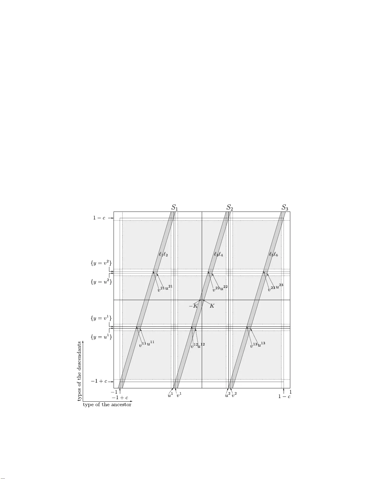
The Annals of Pr ob ability 2011, V ol. 39, No. 2, 549–58 6 DOI: 10.1214 /10-AOP558 c  Institute of Mathematical Statistics , 2 011 THE ALGEBRA IC DIFFERENCE OF TW O RANDOM CANTOR SETS: THE LARSS ON F AMIL Y By Michel Dekking 1 , K ´ arol y Simon 1 , 2 and Bal ´ azs Sz ´ ekel y 3 T e chnic al University of Delft, T e chnic al University of Budap est and T e chnic al University of Budap est In th is pap er, we consider a family of rand om Cantor sets on the line and consider the q uestion of whether the cond ition th at the sum of the Hausdorff dimensions is larg er than one implies the existence of interio r p oints in the difference set of tw o indep endent copies. W e giv e a new and complete proof that this is the case for th e random Can tor sets introduced by P er Larsson. 1. In tro duction. Algebraic differences of Cantor sets o ccur naturally in the context of the dynamical b ehavi or of diffeomorphisms. F rom th ese stud - ies originated a co njecture by Pa lis and T ak ens [ 8 ], relating the s ize of th e arithmetic difference C 2 − C 1 = { y − x : x ∈ C 1 , y ∈ C 2 } to the Hausdorff dimensions of the t wo Can tor s ets C 1 and C 2 : if dim H C 1 + dim H C 2 > 1 , (1) then, generic al ly , it should b e true that C 2 − C 1 con tains an in terv al . F or generic dyn amically generated nonline ar Can tor sets, this wa s pr o ven in 2001 b y de Moreira and Y occoz [ 1 ]. The problem is op en for generic linear Cantor sets. The problem w as put into a probabilistic con text b y P er Larsson in his thesis [ 5 ] (see also [ 6 ]). He considers a t wo-parameter family of Received March 2009; rev ised Marc h 2010. 1 Supp orted in p art by th e NWO-OTKA common pro jec t. 2 Supp orted by OTKA F oun dation #K71693. 3 Supp orted by HSN Lab. AMS 2000 subje ct classific ations. Primary 28A80; secondary 60J80, 60J85. Key wor ds and phr ases. Random fractals, random iterated function systems, differ- ences of Can tor sets, Pa lis conjecture, multit y p e branching processes. This is an electr o nic reprint of the o r iginal article published by the Institute of Mathematica l Statistics in The Annals of Pr ob ability , 2011, V ol. 39 , No. 2, 54 9 –586 . This re pr int differs from the original in pagination and t yp ogr aphic detail. 1 2 M. DEKKING, K. S IMON AND B. SZ ´ EKEL Y Fig. 1. R e gions describ e d by e quations ( 3 ) and ( 4 ) . random Can tor sets C a,b , and claims to pr o ve that the P alis conjecture holds for all relev an t c h oices of the parameters a and b . Although the main idea of Larsson’s argument is brillian t, unfortunately , th e pro of cont ains significan t gaps and in correct reasoning. The aim of the present pap er is to giv e a correct p ro of of this th eorem. The most imp ortant error made by Larsson is as follo ws: during the constru ction, a m ultit yp e br anc hing pro ce ss with uncounta bly many t yp es app ears naturally . The n umber of in dividuals in the n th generatio n having t yp es wh ic h fall into th e set A is denoted Z n ( A ) and the probabilit y measure describin g the branching pro cess starting with a single type- x ind ividual is denoted by P x . Th e argument presented in Larsson’s pap er requires that for some p ositive δ , q , ρ > 1 and for a set A of whic h the interior con tains 0, we hav e that, u niformly , both in x and in n , the follo wing holds : P x ( Z n ( A ) > δ · ρ n ) > q . (2) Ho wev er, the main result in the theory of general multit yp e branc hing pro cesses [ 4 ], Theorem 14.1, in vok ed by Larsson implies ( 2 ) without an y uniformity . F urther (as shown in [ 3 ]), the idea p r esen ted in Larsson’s pap er wo rks only in the region (see also Figure 1 ) where 1 − 4 a − 2 b + 3 a 2 − 6 ab > 0 . (3) Although we use a differen t setup, the main idea pr esen ted here follo ws the line of Larsson’s pro of. THE DIFFERENCE OF RAND OM CAN TOR SETS 3 Fig. 2. The c onstruction of the Cantor set C a,b . The figur e shows C 1 a,b , . . . , C 4 a,b . W e remark that for lin ear Canto r sets of a differen t natur e, the firs t t wo authors inv estigated the s ame pr ob lem in [ 2 ]. F urther devel opments in this direction in [ 7 ] lead us to conjecture that in the critical case, th at is, dim H ( C a,b ) = 1 / 2, the difference set will a.s. cont ain no interv al. 1.1. L arsson ’s r andom Cantor sets. It is assu med thr oughout this pap er that a > 1 4 and 3 a + 2 b < 1 . (4) The first condition is a gro wth condition and since dim H C a,b = − log 2 log a , this cond ition is equ iv alen t to dim H C a,b > 1 / 2, w hic h is equ iv alen t to ( 1 ). The second condition is a geometric condition: Lars son’s C an tor set is a natural randomizatio n of the classical Can tor set; see Figure 2 . In the first step of the construction, interv als of length a are put in to the inte rv als [ b, 1 2 − a 2 ] and [ 1 2 + a 2 , 1 − b ] . Dismissin g th e trivial case 3 a + 2 b = 1 , this ob viously requires 3 a + 2 b < 1 . W e remark that it is useful to force a forbid den zone of length at least a in the mid dle sin ce otherwise the Newhouse thic kness of the Can tor set wo uld b e larger than 1, whic h yields an in terv al in the difference set by Newhouse’s theorem (see [ 8 ], page 63). The tw o in terv als of length a eac h ha ve ro om to mo ve in an in terv al of length 1 2 − a 2 − b , that is, there is a free space of size 1 2 − a 2 − b − a an d we d enote this gap b y g : g := 1 − 3 a − 2 b 2 . The construction is as follo ws: fi rst, remov e th e midd le a part, then the b parts from b oth th e b eginning and the end of the unit in terv al. Then, place in terv als of length a according to a un iform d istribution in the remaining t w o op en spaces [ b, 1 2 − a 2 ] and [ 1 2 + a 2 , 1 − b ] . These tw o ran d omly chosen interv als of length a are called th e level- one intervals of the random Cant or set C a,b . W e write C 1 a,b for their union. In b ot h of the t w o lev el-one in terv als, w e r ep eat the same construction indep enden tly of eac h other and of the previous step. In this wa y , w e obtain f our disjoint interv als of length a 2 . W e emphasize that, b eca use of in dep end ence, th e relativ e p ositi ons of these second lev el 4 M. DEKKING, K. S IMON AND B. SZ ´ EKEL Y in terv als in the fir st lev el ones are, in general, completely different. Similarly , w e construct the 2 n lev el- n inte rv als of length a n . W e call their un ion C n a,b . Larsson’s random Can tor set is then defined b y C a,b := ∞ \ n =1 C n a,b . See Figure 2 . The next theorem w as stated b y P . Larsson. Theorem 1. L et C 1 , C 2 b e indep endent r andom Cantor sets having the same distribution as C a,b define d ab ove. Then, the algebr aic differ e nc e C 2 − C 1 almost sur e ly c ontains an interval. This pap er is organized as follo ws. In the next s ection, w e give an elemen- tary p r o of of the fact th at the p robabilit y that C 2 − C 1 con tains an interv al is either 0 or 1. F or the m ain part of the p r o of, our starting p oin t is the observ ation that C 2 − C 1 can b e view ed as a 45 ◦ pro jection of the pro du ct set C 1 × C 2 . This leads, in Section 3.1 , to th e in tr o duction of the lev el- n squares formed as the pro d uct of lev el- n inte rv als of the Canto r sets C 1 , C 2 . W e remark that Larsson do es not u se these squares at all. Th en, based on the family of th ese squares w e w ill construct the in tr insic branching pro cess and state our Main Lemma , wh ic h will replace ( 2 ). In S ection 4 , w e prov e Theorem 1 , assumin g the Main Lemm a . In Sections 5 – 10 , we giv e a pr o of of the Main Lemma . 2. A 0–1 la w. Undoub tedly , Larsson introdu ced his Canto r sets as a natural r andomization of the classical triadic Can tor set. Actually , these sets can also b e considered as very simp le examples of statistically self-similar sets, whic h p ermits us to giv e a simple p ro of of the 0–1 la w for the int erv al prop erty . A set C is statistic al ly self-similar if there is a collectio n of m random functions { ϕ 1 , . . . , ϕ m } such that C = m [ i =1 ϕ i ( C i ) , where the C i are indep enden t rand om sets with the same distribution as C . F or Larsson’s sets, m = 2 and th e rand om f unctions are the affine fu n ctions ϕ 1 ( x ) = ax + b + U 1 and ϕ 2 ( x ) = ax + (1 + a ) / 2 + U 2 , where U 1 and U 2 are indep endent random v ariables, b oth uniformly dis- tributed o v er [0 , g ]. Pr opos ition 1. P ( C 2 − C 1 ⊃ I ) = 0 or 1 . THE DIFFERENCE OF RAND OM CAN TOR SETS 5 Pr oof. F or 1 ≤ i, j ≤ 2 , let C i,j b e ind ep endent copies of C = C a,b and let C 1 = ϕ 1 ( C 1 , 1 ) ∪ ϕ 2 ( C 1 , 2 ) , C 2 = ϕ 1 ( C 2 , 1 ) ∪ ϕ 2 ( C 2 , 2 ) b e the self-similarit y equations for C 1 and C 2 . W e will also write “ C 2 − C 1 con tains an in terv al” equiv alen tly as “ C 2 − C 1 has nonempt y in terior.” Using the facts that for arbitrary subsets A, B , C and D of R , ( A ∪ B ) − ( C ∪ D ) ⊃ ( A − C ) ∪ ( B − D ) , that ϕ ( A − B ) = ϕ ( A ) − ϕ ( B ) for affin e functions ϕ : R → R and that affine functions are con tinuous, we can set up the follo win g c h ain of (in)equalities: p := P ( C 2 − C 1 ⊃ I ) = 1 − P (Int( C 2 − C 1 ) = ∅ ) ≥ 1 − P (Int( ϕ 1 ( C 2 , 1 ) − ϕ 1 ( C 1 , 1 )) = ∅ , Int ( ϕ 2 ( C 2 , 2 ) − ϕ 2 ( C 1 , 2 )) = ∅ ) = 1 − P (Int( ϕ 1 ( C 2 , 1 ) − ϕ 1 ( C 1 , 1 )) = ∅ ) P ( In t( ϕ 2 ( C 2 , 2 ) − ϕ 2 ( C 1 , 2 )) = ∅ ) = 1 − P (Int( ϕ 1 ( C 2 , 1 − C 1 , 1 )) = ∅ ) P (Int( ϕ 2 ( C 2 , 2 − C 1 , 2 )) = ∅ ) = 1 − P (Int( C 2 , 1 − C 1 , 1 ) = ∅ ) P (Int( C 2 , 2 − C 1 , 2 ) = ∅ ) = 1 − (1 − p ) 2 . This implies that p ≤ p 2 and hence p = 0 or 1.  3. Notatio n and the Main Lemma . In th e r emainder of the pap er, w e fix a pair ( a, b ) s atisfying condition ( 4 ) and alwa ys d eal with Larsson’s Can tor sets, so w e will supp ress the lab els a, b . 3.1. The ge ometry of the algebr aic differ enc e C 2 − C 1 . The 45 ◦ pro jection of a p oint ( x 1 , x 2 ) ∈ R 2 on to the x 2 -axis is denoted b y Pro j 45 ◦ . That is, Pro j 45 ◦ ( x 1 , x 2 ) := x 2 − x 1 . The follo w ing tr ivial fact is the motiv ation for constru cting our branching pro cess of lab eled squares: x ∈ Pro j 45 ◦ ( C 1 × C 2 ) if and only if x ∈ C 2 − C 1 . So, C 2 − C 1 = ∞ \ n =0 Pro j 45 ◦ ( C n 1 × C n 2 ) . W e can naturally lab el the squares in C n 1 × C n 2 as follo ws: w e call the upp er-left first lev el square Q 1 and contin ue lab eling the firs t lev el squares 6 M. DEKKING, K. S IMON AND B. SZ ´ EKEL Y Fig. 3. The first level squar es Q 1 , . . . , Q 4 and four se c ond level squar es Q 21 , Q 22 , Q 23 , Q 24 . Q 2 , Q 3 , Q 4 in the clockwise direction; then, within eac h of these squ ares, w e con tinue in this w a y; see Figure 3 . F or an x ∈ [ − 1 , 1] , w e write e ( x ) f or that line with slop e 1 wh ic h in tersects the v ertical axis at x . As we observ ed ab ov e x ∈ C 2 − C 1 if and only if e ( x ) ∩ ( C 1 × C 2 ) 6 = ∅ . (5) Fix x and an arb itrary n . Let S n b e the set of all a n × a n squares con tained in [0 , 1] 2 . Note that for eve ry Q ∈ S n , by the statistical s elf-similarit y of the construction, the p robabilit y of the ev en t e ( x ) ∩ ( Q ∩ ( C 1 × C 2 )) 6 = ∅ conditional on Q ⊂ C n 1 × C n 2 is equal to the probability of the even t e (Φ) ∩ ( C 1 × C 2 ) 6 = ∅ , wh ere we construct Φ = Φ( Q, x ) as follo ws: w e rescale th e square Q (whic h is an a n × a n square) b y the factor 1 /a n , then w e c ho ose Φ su c h that the line segment e (Φ) ∩ [0 , 1] 2 is the rescaled cop y of e ( x ) ∩ Q ; see Figure 4 . More pr ecisely , if ( u, v ) is the low er-left corner of Q , that is, Q = [ u, u + a n ] × [ v , v + a n ], then we d efine Φ( Q, x ) := ( u − v + x a n , if e ( x ) in tersects Q , Θ , otherwise, (6) where Θ is a symbol representing the emptiness of the in tersection. Obser ve that Φ( Q, x ) > 0 if and only if the cen ter of Q is lo cated b elo w the line e ( x ) THE DIFFERENCE OF RAND OM CAN TOR SETS 7 Fig. 4. A level- n squar e Q and its r esc ale d typ e Φ( Q, x ) . and e ( x ) m eets Q . F urther, Φ( Q, x ) = 1 if e ( x ) inte rsects Q at the upp er-left corner and Φ( Q, x ) = − 1 if e ( x ) in tersects Q at the lo wer-righ t corner. 3.2. The pr ob ability sp ac e . W e wr ite T := S ∞ n =0 { 1 , 2 } n for the dya dic tree, w ith no d es i n = i 1 i 2 . . . i n , where i k is 1 or 2 , and ro ot Λ. F or th e construction of Larsson’s Can tor set, the p robabilit y space is Ω 1 = [0 , g ] T [recall that g = (1 − 3 a − 2 b ) / 2]. An elemen t of Ω 1 is denoted b y U , that is, the v alue at the nod e i 1 i 2 . . . i n is U i 1 i 2 ...i n . The corresp onding σ -a lgebra is B 1 := Q T B [0 , g ]. Finally , the probabilit y measure for Larsson’s Cant or set is P 1 := δ 0 × Y T \{ Λ } Uniform[0 , g ] , where δ 0 is the Dirac mass at 0 associated with the mass at the ro ot Λ . Note that the randomness starts at lev el 1. So, the probabilit y space for C 1 × C 2 is as follo ws: Ω := Ω 1 × Ω 1 , B := B 1 × B 1 , P := P 1 × P 1 . (7) An element of Ω is a pair of lab eled binary tr ees. T he 4 n lev el- n pairs of in dices ( i 1 i 2 . . . i n , j 1 j 2 . . . j n ) are natur ally asso ciated with leve l- n squares Q ′ ( i 1 i 2 ...i n ,j 1 j 2 ...j n ) of size a n × a n whose relativ e p ositions are giv en b y U i 1 i 2 ...i n and U j 1 j 2 ...j n . Note, ho wev er, that (to simplify the notation) w e ha v e give n new indices to these squares and p ositions: Q 1 := Q ′ 1 , 2 , Q 2 := Q ′ 2 , 2 , Q 3 := Q ′ 2 , 1 , Q 4 := Q ′ 1 , 1 and similarly f or higher ord er squares and their p ositions (see Figure 3 ). 8 M. DEKKING, K. S IMON AND B. SZ ´ EKEL Y 3.3. The br anching pr o c ess. On the probability space Ω , w e defi n e a m ul- tit yp e branc hing pro cess Z = ( Z n ) ∞ n =0 . F or a Borel set A, the natural num b er Z n ( A ) represents th e num b er of ob jects in generation n whose t yp e falls into the set A . The typ e sp ace T is a su bset of [ − 1 , 1], but for the moment w e can think of T = [ − 1 , 1]. The ob jects of the n th generation are squares Q ∈ S n and, giv en a fixed x ∈ [ − 1 , 1], their t yp e is Φ( Q, x ) , as defin ed in ( 6 ). Note that although w e sp eak of Θ as a type, it is not an elemen t of T . The pr o cess ( Z n ) is a Mark ov chain whose states are collect ions of squares lab eled by their types. The transition mec hanism is as describ ed in Section 3.1 . The initial cond ition of the chain is the square [0 , 1] × [0 , 1], with t yp e x (also called the anc estor of th e br anc hing pro cess). As usu al, we then w rite, for n ≥ 1 , P x ( Z n ( A 1 ) = r 1 , . . . , Z n ( A k ) = r k ) = P ( Z n ( A 1 ) = r 1 , . . . , Z n ( A k ) = r k |Z 0 ( { x } ) = 1) for all k ≥ 1 , A 1 , . . . , A k ⊂ T and nonnegativ e inte gers r 1 , . . . , r k . A collection of squares all w ith typ e Θ is an absorb ing state: it only generates squares with t yp e Θ. This is ob v ious f rom th e defi nition of Φ( Q, x ) , but we w ill extend this pr op ert y to the case of smaller type sp aces T , wh ere, b y definition, a square has type Θ if its t yp e is not in T (this will b e further explained in Section 6.1 ). A ma jor role in our analysis is pla y ed b y the expectations E x [ Z n ( A )] for A ⊂ T , n ≥ 1. Let us defin e, for i = 1 , 2 , 3 , 4 , Z i 1 ( A ) =  1 , if Φ( Q i , x ) ∈ A , 0 , otherwise. (8) Then, Z 1 ( A ) = Z 1 1 ( A ) + · · · + Z 4 1 ( A ) and so E x [ Z 1 ( A )] = Z Ω Z 1 ( A ) d P x = Z Ω 4 X i =1 Z i 1 ( A ) d P x = 4 X i =1 P x (Φ( Q i , x ) ∈ A ) = 4 X i =1 Z A f x,i ( y ) d y , where the f x,i are the densities of the rand om v ariables Φ( Q i , x ) (apart from an atom in Θ ). In Section 5.2 , these densities will b e determined explicitly . It follo ws that for n = 1 , M n ( x, A ) := E x [ Z n ( A )] has a densit y m 1 ( x, y ), called the kernel of the branching pr o cess, giv en by m ( x, y ) := m 1 ( x, y ) = 4 X i =1 f x,i ( y ) . (9) THE DIFFERENCE OF RAND OM CAN TOR SETS 9 W e remark that if M 1 has a d ensit y , then M n also h as a den sit y . Let us write m n ( x, · ) for the densit y of M n ( x, · ) . The branching str ucture of Z yields (see [ 4 ], page 67) m n +1 ( x, y ) = Z T m n ( x, z ) m 1 ( z , y ) d z . (10) The main p roblem to b e solv ed is that the natural c hoice of T = [ − 1 , 1] as t y p e s pace d o es not w ork b ecause of condition (C) b elo w and b eca use we need the uniformity alluded to in equation ( 2 ). Since the definition of T is complicated, we p ostp one it to S ection 6 . Ho wev er, here w e collect the most imp ortan t pr op erties of T : (A) T is the disjoint un ion of finitely man y closed interv als; (B) ther e exists a K > 0 suc h that [ − K, K ] ⊂ T ; (C) the k ernel m n ( x, y ) d efined in ( 10 ) is uniformly p ositiv e on T × T [see cond ition ( C1 ) b elo w] and it h as Perron–F robeniu s eigen v alue greater than 1 [see condition ( C2 ) b elo w]. 3.4. The asym ptotic b ehavior of the br anching pr o c ess Z . W e will pr o ve in Sections 6 , 7 and 8 that there exists an intege r n 0 suc h that m n 0 is a uniformly b ound ed f u nction, that is, there exist 0 < a min < a max suc h that for all x, y ∈ T , we ha ve 0 < a min ≤ m n 0 ( x, y ) ≤ a max < ∞ . (C1) In the next step, w e consider the follo wing t wo oper ators: g ( x ) 7→ Z R m 1 ( x, y ) · g ( y ) d y , h ( y ) 7→ Z R h ( x ) · m 1 ( x, y ) d x . (11) W e cite the follo wing theorem fr om [ 4 ], Theorem 10.1. Theorem 2 (Harris). It fol lows fr om ( C1 ) that the op er ators in ( 11 ) have a c ommon dominant eig envalue ρ . L et µ ( x ) and ν ( y ) b e the c orr e- sp onding eigenfunctions of the first and se c ond op er ator in ( 11 ), r esp e c- tively. Then, the fu nctions µ ( x ) and ν ( y ) ar e b ounde d and uniformly p os- itive. Mor e over, ap art fr om a sc aling, µ and ν ar e the onl y nonn e gative eigenfunctions of these op er ators. F urther, if we norm alize µ and ν so that R µ ( x ) ν ( x ) d x = 1 , which wil l b e henc eforth assume d, then, for al l x, y ∈ T , as n → ∞ ,     m n ( x, y ) ρ n − µ ( x ) ν ( y )     ≤ C 1 µ ( x ) ν ( y )∆ n , wher e the b ound ∆ < 1 c an b e taken indep endently of x and y , a nd the c onstant C 1 is indep endent of x, y and n . 10 M. DEKKING, K. S IMON AND B. SZ ´ EKEL Y Later in this pap er, w e will pr o ve that in ou r case , this P erron–F rob enius eigen v alue is greater than one: ρ > 1 . (C2) Using Theorem 2 , Harris prov es that Z n ( A ) in fact gro ws exp on entially with rate ρ . I ntro ducing W n ( A ) := Z n ( A ) ρ n , he obtains (see [ 4 ], Theorem 14.1 ) th e f ollo wing result. Theorem 3 (Ha rris). If sup x ∈ T E x [ Z 1 ( T ) 2 ] < ∞ , (C3) then it fol lows fr om ( C1 ) and ( C2 ) tha t for al l x ∈ T , P x  lim n →∞ W n ( A ) = : W ( A )  = 1 . (12) F urther, for every Bor el me asur able A ⊂ T with L eb 1 ( A ) > 0 , we ha ve P x ( W ( A ) > 0) > 0 . (13) Mor e over, let A and B b e su b sets of T such that their L eb esgue me asur es ar e p ositive. Then, the r elation W ( B ) = R B ν ( y ) d y R A ν ( y ) d y W ( A ) holds P x almost sur ely for an y x ∈ T . W e are go ing to use this theorem to prov e our Main Lemma , whic h summarizes ev erything we need concerning our branching pro cess. Roughly sp eaking, the Main Lemm a sa ys th at for the br anc hing p ro cess asso ciated to Larsson’s Canto r set, the statemen t in Theorem 3 h olds u niformly both in n and x for an app ropriately c hosen small in terv al of x ’s. Main Le mma. Ther e exist p ositive numb ers δ and q , an N ∈ N and a smal l interval [ − K, K ] ⊂ T c enter e d at the origin such that the f ol lowing ine quality holds: inf n ≥ N inf x ∈ [ − K ,K ] P x ( Z n ([ − K, 0]) > δ ρ n , Z n ([0 , K ]) > δ ρ n ) ≥ q . (14) 4. The pro of of Theorem 1 . In Section 3.1 , w e defin ed the t yp e of a square Q b y means of its intersect ion with a line e ( x ). Here, w e will elab orate on this in tersection. THE DIFFERENCE OF RAND OM CAN TOR SETS 11 4.1. Nic e i nterse ction of a squar e with a line e ( x ) . W e sa y th at a squ are Q has a nic e interse ction with e ( x ) if Φ( Q, x ) ∈ [ − K, K ] , where K comes from Main Lemma . F or s mall K, this means that the cen ter of Q is close to the line e ( x ). Let A 0 = { [0 , 1] 2 } , A n b e the set { Q ∈ S n : Q ⊂ C n 1 × C n 2 } and A n x b e the set of squares from A n ha ving nice in tersection with e ( x ). That is, for x ∈ T and n ≥ 1 , w e d efine A n x := { Q ∈ A n : | Φ( Q, x ) | ≤ K } . Moreo ve r, for m ≥ 0 and a square Q ∈ A m x , we w rite l + n ( Q, x ) and ( l − n ( Q, x ) ) for the n um b ers of lev el-( m + n ) squares conta ined in Q whic h ha ve nice in tersection with e ( x ) with cen ter b elo w an d ab o v e the line e ( x ) , resp ectiv ely . That is, for a Q = Q i 1 ...i m , let l + n ( Q, x ) = # { Q i 1 ...i m j 1 ...j n ∈ A m + n : 0 ≤ Φ ( Q i 1 ...i m j 1 ...j n , x ) ≤ K } . Similarly , let l − n ( Q, x ) = # { Q i 1 ...i m j 1 ...j n ∈ A m + n : − K ≤ Φ ( Q i 1 ...i m j 1 ...j n , x ) ≤ 0 } . Finally , for ev ery n ≥ 1 , x ∈ T and Q ∈ A m x , w e d efine the ev ent A n ( Q, x ) := { l − n ( Q, x ) > δ ρ n , l + n ( Q, x ) > δ ρ n } , where δ comes from th e Main Lemma . Note that the self-similarit y of the construction of the squares and the Main Lemma for the und er lyin g branch- ing pro cess imply the follo wing: for n ≥ N and a square Q ∈ S m , w e ha ve P ( A n ( Q, x ) | Q ∈ A m x ) (15) = P Φ( Q,x ) ( Z n ([ − K, 0]) > δ ρ n , Z n ([0 , K ]) > δ ρ n ) ≥ q . 4.2. The differ enc e set C 2 − C 1 c ontains an interval with p ositive P pr ob- ability. W e in tro d uce the in terv al I := [ − K a N , K a N ] with N and K f rom the Main Lemma . Note that | I | := L eb 1 ( I ) = 2 K a N . Our goal is to pro v e that P ( C 2 − C 1 ⊃ I ) > 0 . First, we divide the int erv al I in to 4 2 N in terv als I i 1 of equal lengt h with indices ± 1 , . . . , ± 1 2 4 2 N . Then, w e divide all of these interv als in to 4 3 N in- terv als I i 1 i 2 of equal length. If w e hav e already defined the ( k − 1)th lev el in terv als, then we define the k th lev el in terv als I i 1 ...i k b y sub dividing eac h 12 M. DEKKING, K. S IMON AND B. SZ ´ EKEL Y ( k − 1)th level int erv al I i 1 ...i k − 1 in to 4 ( k +1) N in terv als of equal length with indices ± 1 , . . . , ± 1 2 4 ( k +1) N . W e denote the cen ter of I i 1 ...i k b y z i 1 ...i k . That is, I i 1 ...i k = [ z i 1 ...i k − K a N 4 − [2+ ··· +( k +1)] N , z i 1 ...i k + K a N 4 − [2+ ··· +( k +1)] N ] , where the z i 1 ...i k are equally spaced in I i 1 ...i k − 1 . Note that the in terv al I i 1 ...i k has length | I i 1 ...i k | = 2 K a N 4 − [2+ ··· +( k +1)] N < 2 K a g k , (16) where w e put g k := (1 + · · · + ( k + 1)) N = 1 2 ( k + 1)( k + 2) N . In the follo win g, we will go from generation g k − 1 to generation g k . Definition 1. W e sa y that the eve nt B k ( z i 1 ...i k ) o ccurs if ther e exists some square Q ∈ A g k − 1 , itself h a vin g nice intersect ion with e ( z i 1 ...i k ), suc h that A ( k +1) N ( Q, z i 1 ...i k ) holds—cf. Figure 5 . In form u lae, B k ( z i 1 ...i k ) = [ Q ∈A g k − 1 z i 1 ...i k A ( k +1) N ( Q, z i 1 ...i k ) . (17) The follo wing lemma is one of the key stat emen ts of the argument. Lemma 1. Assume that B k ( z i 1 ...i k ) o c cu rs with the squar e Q . L et Q + and Q − b e the c ol le ctions of level- g k squar es within Q having nic e interse ction with e ( z i 1 ...i k ) with c enter b elow and ab ove the line e ( z i 1 ...i k ) , r esp e ctively. Then, (1) Pro j 45 ◦  [ e Q ∈Q + e Q  ⊃ I i 1 ...i k , Pro j 45 ◦  [ e Q ∈Q − e Q  ⊃ I i 1 ...i k . (2) F or every i k +1 = ± 1 , . . . , ± 1 2 4 ( k +2) N , the line e ( z i 1 ...i k i k +1 ) has nic e in- terse ction with al l squar es fr om either Q + or Q − . Thus, the line e ( z i 1 ...i k i k +1 ) has nic e interse ction with at le ast δ ρ ( k +1) N squar es c ontaine d in Q such that either al l have c enter b elow the line e ( z i 1 ...i k ) or al l have c enter ab ove the line e ( z i 1 ...i k ) . Pr oof. Cho ose an arbitrary y ∈ I i 1 ...i k . Without loss of generalit y , we ma y assume that y ≤ z i 1 ...i k . Then, to sho w b oth (1) and (2), it is enough to pro v e that e ( y ) has nice in tersection w ith all squares from Q + . THE DIFFERENCE OF RAND OM CAN TOR SETS 13 Fig. 5. Event B k ( z i 1 ...i k ) : ther e is a level- g k − 1 squar e Q i n which the numb er of strip e d level- g k squar es (the nic ely interse cting ones) is at le ast δ ρ N ( k +1) , b oth for the squar es with c enter ab ove and the squar es with c enter b el ow the li ne e ( z i 1 ...i k ) . Fig. 6. Nic e inters e ctions. Fix an arbitrary Q ∈ Q + . By the d efinition of Q + , the square Q is a lev el- g k square suc h th at its lo we r-left corner is in b et wee n th e parallel lines e ( z i 1 ...i k ) and e ( z i 1 ...i k − K a g k ). So, f or ev ery p oint y ∗ ∈ [ z i 1 ...i k − K a g k , z i 1 ...i k ] , the line e ( y ∗ ) has nice int ersection with Q ; see Fig ure 6 . T o show that for any y ∈ I i 1 ...i k ∩ ( −∞ , z i 1 ...i k ] , e ( y ) has nice in tersection with all squares from Q + , it is enough to pro v e that I i 1 ...i k ∩ ( −∞ , z i 1 ...i k ] ⊂ [ z i 1 ...i k − K a g k , z i 1 ...i k ] , 14 M. DEKKING, K. S IMON AND B. SZ ´ EKEL Y based on the previous paragraph. Ho wev er, since | I i 1 ...i k ∩ ( −∞ , z i 1 ...i k ] | = 1 2 | I i 1 ...i k | < K a g k , this follo w s using ( 16 ).  Definition 2. Let E 0 := A N ([0 , 1] 2 , 0) and let E k := T i 1 ...i k B k ( z i 1 ...i k ) . Lemma 2. The fol lowing ine quality holds: P ( C 2 − C 1 ⊃ I ) ≥ q Y k ≥ 1 P ( E k | E k − 1 ) . (18) Pr oof. Using the fact that I = [ − K a N , K a N ] = S i 1 ...i k I i 1 ...i k , it follo ws immediately from Lemma 1 that if the ev ent E k holds, then the ev ent S k := { Pro j 45 ◦ ( C g k 1 × C g k 2 ) ⊃ I } will hold. Th erefore, E k ⊂ S k . Since the sets C g k 1 × C g k 2 are decreasing, we obtain that S k ⊃ S k +1 . Thus, P ( C 2 − C 1 ⊃ I ) = P  \ k ≥ 1 S k  = lim k →∞ P ( S k ) ≥ inf k ≥ 1 P ( E k ) ≥ P ( E 0 ) Y k ≥ 1 P ( E k | E k − 1 ) . The last inequalit y holds since P ( E 0 ) Y i ≥ 1 P ( E i | E i − 1 ) ≤ P ( E 0 ) P ( E 1 | E 0 ) · · · P ( E k | E k − 1 ) = p P ( E k E k − 1 ) ≤ P ( E k ) , where p = P ( E 0 ) P ( E 0 ) P ( E 1 E 0 ) P ( E 1 ) · · · P ( E k − 1 E k − 2 ) P ( E k − 1 ) ≤ 1 . Since the Main Lemma yields P ( E 0 ) ≥ q , one obtains the statemen t of th e lemma.  In Lemma 3 , w e giv e a lo we r b ound for P ( E k | E k − 1 ) for ev ery k . Lemma 3. F or any k ≥ 1 , we ha ve P ( E k | E k − 1 ) ≥ 1 − 4 2 N + ··· +( k + 1) N (1 − q ) δρ kN . THE DIFFERENCE OF RAND OM CAN TOR SETS 15 Pr oof. W e recall that E k w as defined as E k := \ i 1 ...i k B k ( z i 1 ...i k ) . Therefore, we hav e to prov e that P  [ i 1 ...i k B c k ( z i 1 ...i k )    E k − 1  ≤ 4 2 N + ··· +( k + 1) N (1 − q ) δρ kN . Note that the num b er of indices i 1 . . . i k on the left-hand side is equal to 4 2 N + ··· +( k + 1) N . Th er efore, it is enough to show that for eac h index i 1 . . . i k , w e ha v e P ( B c k ( z i 1 ...i k ) | E k − 1 ) ≤ (1 − q ) δρ kN . By Definition 1 , to see this, w e ha ve to pro ve that P  \ Q ∈A g k − 1 z i 1 ...i k A c ( k +1) N ( Q, z i 1 ...i k )    E k − 1  ≤ (1 − q ) δρ kN . (19) W e assume E k − 1 , so, in p articular, w e kno w that B k − 1 ( z i 1 ...i k − 1 ) holds. That is, there exists a leve l- g k − 2 square Q big suc h that the ev en t A k N ( Q big , z i 1 ...i k − 1 ) holds. By d efinition, this means that we can fi nd at lea st [ δ ρ k N ] + 1 squares in Q big in A g k − 1 z i 1 ...i k − 1 ha ving center b elo w, and at least as many squ ares ha v- ing cen ter ab ov e, the line e ( z i 1 ...i k − 1 ). Using the second part of Lemma 1 (for k instead of k + 1 ), we obtain that the line e ( z i 1 ...i k ) has nice in tersec- tion with either all th e squares ab ov e or with all the squares b elo w the line e ( z i 1 ...i k − 1 ). Without loss of generalit y , we ma y assume the former. Ho wev er, for all these squares Q , the ev ents A c ( k +1) N ( Q, z i 1 ...i k ) are (con- ditionally) indep enden t, so, to obtain ( 19 ), it is enough to sho w that P ( A c ( k +1) N ( Q, z i 1 ...i k ) | Q ∈ A g k − 1 z i 1 ...i k ) ≤ 1 − q (20) and this follo ws directly from equation ( 15 ).  Lemma 4. F or al l n ≥ 1 , we have ∞ Y j =1 (1 − 4 [2+ ··· +( j +1)] n (1 − q ) δρ j n ) > 0 . (21) Pr oof. W e hav e to sh o w that P ∞ j =1 a j con verges, where a j = 4 (1 / 2) j ( j +1) n (1 − q ) δρ j n . It is therefore sufficien t that a j ≤ e − j for all large j . This is true since 16 M. DEKKING, K. S IMON AND B. SZ ´ EKEL Y 1 j log a j = 1 2 ( j + 1) n log 4 + 1 j δ ( ρ n ) j log(1 − q ) ≤ − 1 , whic h holds for j large enough since ρ n > 1 and log(1 − q ) < 0 .  Therefore, using Lemmas 2 , 3 an d 4 , w e obtain that P ( C 2 − C 1 ⊃ I ) ≥ q ∞ Y k =1 (1 − 4 [2+ ··· +( k +1)] N (1 − q ) δρ kN ) > 0 . Com bining this with Prop osition 1 from Section 2 , this completes the pr o of of Theorem 1 . In the next six sectio ns, w e p r o ve our Main Lemma . 5. Distribution of types. In this section, the densit y fu nction of Φ( Q, x ) will b e determined for the four squares Q fr om S 1 . 5.1. The distribution of Φ( Q, x ) . Let U 1 , U 2 , U 3 , U 4 b e four indep endent Uniform([0 , g ])-distributed random v ariables. Th e left corners of the t wo lev el-one in terv als of the random C an tor set C i are d etermined by U 2 i − 1 , U 2 i for i = 1 , 2. Let ( u i , v i ) b e the lo wer-left corner of the squares Q i , i = 1 , . . . , 4 (see Figure 7 ). Then, ( u 1 , v 1 ) =  b + U 1 , 1 2 + a 2 + U 4  , ( u 2 , v 2 ) =  1 2 + a 2 + U 2 , 1 2 + a 2 + U 4  , ( u 3 , v 3 ) =  1 2 + a 2 + U 2 , b + U 3  , ( u 4 , v 4 ) = ( b + U 1 , b + U 3 ) . F or an x ∈ [ − 1 , 1] , w e define Φ i ( x ) := Φ ( Q i , x ). F rom ( 6 ), simple compu- tations yield Φ 1 ( x ) =            1 a  − 1 2 − a 2 + b + U 1 − U 4 + x  , if 1 a  − 1 2 − a 2 + b + U 1 − U 4 + x  ∈ [ − 1 , 1] , Θ , otherwise , (22) Φ 2 ( x ) = ( 1 a ( U 2 − U 4 + x ) , if 1 a ( U 2 − U 4 + x ) ∈ [ − 1 , 1] , Θ , otherwise THE DIFFERENCE OF RAND OM CAN TOR SETS 17 Fig. 7. I f x is an element of the b old vertic al li ne, then the li ne e ( x ) interse cts exactly two squar es. If x is an element of one of the two plain vertic al lines, then e ( x ) interse cts one squar e. If x is an element of one of the four dotte d vertic al lines, then e ( x ) i nterse cts at most one squar e. If x is such that a ≤ x ≤ 1 − 2 a − 2 b or − 1 + 2 a + 2 b ≤ x ≤ − a, then e ( x ) interse cts at most two squar es wi th pr ob ability one. If x is such that − 1 2 + 5 a 2 + b ≤ x ≤ a or − a ≤ x ≤ 1 2 − 5 a 2 − b, then e ( x ) interse cts exactly two squar es. and, similarly , Φ 3 ( x ) =            1 a  1 2 + a 2 − b + U 2 − U 3 + x  , if 1 a  1 2 + a 2 − b + U 2 − U 3 + x  ∈ [ − 1 , 1] , Θ , otherwise , 18 M. DEKKING, K. S IMON AND B. SZ ´ EKEL Y Fig. 8. The supp ort of the density functions in the sim ple c ase. (23) Φ 4 ( x ) = ( 1 a ( U 1 − U 3 + x ) , if 1 a ( U 1 − U 3 + x ) ∈ [ − 1 , 1] , Θ , otherwise . T o get a b etter geometric understand ing of the distribu tion of the rand om v ariables Φ i ( x ) , we define the three slan ted strip es S k , k = 1 , 2 , 3 (see Figure 8 ), in suc h a wa y that S k ⊂ [ − 1 , 1] 2 is b ound ed b y th e lines ℓ 2 k − 1 , ℓ 2 k , w here ℓ 1 ( x ) = 1 a x + 1 a (1 − a − 2 b ) , ℓ 2 ( x ) = 1 a x + 2 , ℓ 3 ( x ) = 1 a x + g a , (24) ℓ 4 ( x ) = 1 a x − g a , ℓ 5 ( x ) = 1 a x − 2 , ℓ 6 ( x ) = 1 a x − 1 a (1 − a − 2 b ) . An immediate calculat ion sho w s that the follo wing resu lt h olds. Lemma 5. F or every x ∈ [ − 1 , 1] and e v ery i = 1 , . . . , 4 , if Φ i ( x ) 6 = Θ , then ( x, Φ i ( x )) ∈ S 1 ∪ S 2 ∪ S 3 . THE DIFFERENCE OF RAND OM CAN TOR SETS 19 Let us call ℓ j the graph of the fu nction ℓ j ( x ). Observe that the reflection in the origin of ℓ j is ℓ 7 − j for j = 1 , . . . , 6. F or a p oint ( x 1 , x 2 ) ∈ R 2 , we write π m ( x 1 , x 2 ) := x m , m = 1 , 2. W e then defin e c > 0 by − 1 + c := π 1 ( ℓ 1 ∩ { y = x } ) and obtain c = 2 b 1 − a . By symmetry , it follo ws th at 1 − c = π 1 ( ℓ 6 ∩ { y = x } ) . Using the fact th at − 1 + 2 b = π 1 ( ℓ 1 ∩ { y = − 1 } ) , it follo ws f rom th e symmetry men tioned ab o v e th at x / ∈ ( − 1 + 2 b, 1 − 2 b ) (25) = ⇒ e ( x ) do es not in tersect an y lev el-one square . The functions ℓ 1 ( x ), ℓ 6 ( x ) hav e rep elling fixed p oint − 1 + c , 1 − c, resp ec- tiv ely . Therefore, x ∈ [ − 1 , − 1 + c ) ∪ (1 − c, 1] (26) = ⇒ ∃ n suc h that ( x ) ∩ Q = ∅ for all Q ∈ S n . With pr obabilit y 1 , no line e ( x ) can in tersect more than t w o d escendan ts, in fact, [ − 1 + 2 b, 1 − 2 b ] can b e partitioned in to five sets, according to whic h descendan ts can b e pro du ced, give n b y (see also Figure 7 ) A − 1 =  − 1 + 2 b, − 1 2 + a 2 + b  , A + 1 =  1 2 − a 2 − b, 1 − 2 b  , A − 2 =  − 1 2 + a 2 + b, − a  , A + 2 =  a, 1 2 − a 2 − b  , (27) A 3 =  − a, a  . Lemma 6. If x ∈ A 3 , then x c an only pr o duc e desc endants with typ e Φ 2 ( x ) and/or Φ 4 ( x ) . If x ∈ A + 1 (r esp. x ∈ A − 1 ), then x c an pr o duc e at most one desc endant with typ e Φ 1 ( x ) [ r e sp. Φ 3 ( x ) ]. If x ∈ A + 2 , then ther e ar e two p ossibilities. First, if x pr o duc es Φ 1 ( x ) , then Φ 2 ( x ) and Φ 4 ( x ) c annot b e b orn. Se c ond, if x pr o duc es any of Φ 2 ( x ) and Φ 4 ( x ) , then Φ 1 ( x ) c annot b e b orn. If x ∈ A − 2 , then ther e ar e two similar p ossibilities. Pr oof. In Figure 7 , observe that Pro j 45 ◦ ( Q 1 ) ∩ Pro j 45 ◦ ( Q 4 ) 6 = ∅ can happ en only in the extreme situation if the b ottom of the s q u are Q 1 is the same as the b otto m of the dotted square w hic h con tains Q 1 on Figure 3 . This means that U 4 = 0 , whic h happ en s with probabilit y zero. Similarly , Pro j 45 ◦ ( Q 3 ) ∩ Pro j 45 ◦ ( Q 4 ) 6 = ∅ happ en s only if U 2 = 0 , whic h also has prob- abilit y zero. Pro j 45 ◦ ( Q 1 ) ∩ Pro j 45 ◦ ( Q 3 ) = ∅ alwa ys holds, which completes the pro of of our lemma.  20 M. DEKKING, K. S IMON AND B. SZ ´ EKEL Y 5.2. The density functions. In th is su bsection, we will d etermine the den- sit y f u nctions f Φ i ( x ) ( y ) of the ran d om v ariables Φ i ( x ), i = 1 , 2 , 3 , 4 , giv en explicitly by ( 22 ) and ( 23 ). W e do n ot call them pr ob ability densit y func- tions since the Φ i ( x ) ma y b e equal to Θ with p ositiv e probabilit y for some x . The p robabilit y d ensit y fu nction of the d ifference of tw o ind ep enden t Uniform([0 , g ])-distributed ran d om v ariables is the triangular distribution giv en b y f △ ( z ) = 0 if | z | > g and for 0 ≤ | z | ≤ g b y f △ ( z ) = 1 g 2 ( g − | z | ) . (28) T o get f Φ i ( x ) ( y ) , we apply simple transformations to f △ ( z ) and fi nd f Φ i ( x ) ( y ) = af △ ( ay + c i − x ) 1 [ − 1 , 1] ( y ) (29) with c 1 = − c 3 = 1 2 + a 2 − b and c 2 = c 4 = 0 . F rom the definition, P (Φ i ( x ) = Θ) = 1 − Z [ − 1 , 1] f Φ i ( x ) ( y ) d y . 6. A uniformly p osit iv e k ernel. Here, and in the next tw o sections, we are going to define the t yp e space T of the branc hing pro cess introd u ced in Section 3.3 . In order to ensure that cond itions ( C1 ), ( C2 ), ( C3 ) of Sectio n 3.4 h old, w e intro d uce a typ e space T whic h also satisfies pr op erties (A), (B), (C) of Section 3.3 . It follo ws from ( 26 ) that w e must c ho ose our type space T ⊂ [ − 1 + c, 1 − c ]. Unfortunately , the construction of the type space T satisfying the ab o v e conditions is qu ite inv olve d and tec hnical for those v alues of the p arameters a, b which do not satisfy ( 3 ). Th erefore, w e split the pr esen tation int o tw o parts. In th is s ection, we present the construction of T across three lemmas: Lemmas 7A , 8A and 9A . I n the n ext section, we present the general case with the corresp ond ing Lemmas 7 , 8 and 9 . The main d ifference b et w een these lemmas lies in the pro ofs of Lemmas 7 and 7A . Lemma 8 is almost the same as Lemma 8A . Finally , the pro of of Lemma 9 follo ws the same line as the pro of of Lemma 9A , but is more tec hnical. 6.1. Desc endant distr ibutions and the kernel of the br anching pr o c ess. W e introd uce the random v ariables X 1 ( x ) , X 2 ( x ) , X 3 ( x ) , X 4 ( x ) for 1 ≤ i ≤ 4 b y X i ( x ) =  Φ i ( x ) , if Φ i ( x ) ∈ T , Θ , otherwise. (30) So, the densit y of X i ( x ) is f x,i ( y ) := f Φ i ( x ) ( y ) 1 T ( y ) (31) THE DIFFERENCE OF RAND OM CAN TOR SETS 21 for i = 1 , . . . , 4. In general, X i ( x ) also has an atom: P ( X i ( x ) = Θ) = 1 − R T f x,i ( y ) d y . Recall [see equatio n ( 9 )] that the ke rnel of the branc h ing pr o cess can b e expressed as the sum of the d ensit y functions of the random v ariables X i ( x ), i = 1 , . . . , 4 : m ( x, y ) = f x, 1 ( y ) + f x, 2 ( y ) + f x, 3 ( y ) + f x, 4 ( y ) . The structure of the su pp ort of this k ern el is v ery imp ortan t for the sequel. Since the fu nctions f x,i ( y ) ( i = 1 , 2 , 3 , 4) are piecewise con tin uous on [ − 1 , 1], m ( · , · ) is piecewise cont inuous on [ − 1 , 1] × [ − 1 , 1]. The supp ort of m ( · , · ) is a subset of the th ree slan ting strip es S k , k = 1 , 2 , 3 , introdu ced earlier; see also Figure 8 . Fig. 9. Some p oints and lines r elate d to the kernel m ( x, y ) i f l = 1 . 22 M. DEKKING, K. S IMON AND B. SZ ´ EKEL Y 6.2. The p ossible holes in the supp ort of the ke rnel of Z . W e ha v e seen in ( 26 ) that the b ranc hing p ro cess with ancestor typ e in the set [ − 1 , − 1 + c ] or [1 − c, 1] dies out in a finite n umber of generations almost su rely . Therefore, it is r easonable to restrict the t yp e space to [ − 1 + c + ε, 1 − c − ε ] for some small p ositiv e ε . How ev er, in some cases, we ha v e to mak e fu rther restrictions. Namely , for i = 1 , 2 , we d efine u i := π 1 ( ℓ 2 i ∩ { y = 1 − c } ) , v i := π 1 ( ℓ 2 i +1 ∩ { y = − 1 + c } ); (32) see Figure 8 . Clearly , u 1 − v 1 = u 2 − v 2 and an easy calcula tion sho ws that v 1 < u 1 ⇐ ⇒ c < g 2 a . (33) W e remark that this condition is equiv alent to the condition in equation ( 3 ) (see also Figure 1 ). On the other hand, if u i < v i , i = 1 , 2 , holds, then, for x ∈ [ u i , v i ] , the set E 1 ( x ) := { y : m ( x, y ) > 0 } (34) is con tained in [ − 1 , − 1 + c ] ∪ [1 − c, 1]. This implies that the pro cess dies out in fi nitely many steps for x ∈ [ u i , v i ] (see Figure 9 ). Th erefore, if the condition stated in ( 33 ) d o es not hold, then we hav e to mak e more r estrictions on our t y p e space [ − 1 + c + ε, 1 − c − ε ]. Th is is wh at we are going to do in Section 8 . F o r the con venience of the reader, in Sectio n 7 , w e treat the simpler case when ( 33 ) holds. 7. A un iformly p ositiv e kernel in the simple case. In the remainder of this section, we will pro ve that if ( 33 ) holds, that is, v 1 < u 1 , then we ca n c h o ose a sufficien tly sm all ε 0 > 0 s u c h that T = [ − 1 + c + ε 0 , 1 − c − ε 0 ] satisfies conditions ( C1 ), ( C2 ) and ( C3 ) [and also prop er ties (A), (B), (C)]. The k ernel in the simple case is illustrated in Figure 8 . Lemma 7A. Assume that v 1 < u 1 . Fix an ε > 0 satisfying ε < g 2 a − c. (35) F urther, in this simpler c ase, let T = T ( ε ) = [ − 1 + c + ε, 1 − c − ε ] . (36) Then, the kernel m ( x, y ) of the br anching pr o c ess Z has the fol low ing pr op- erty: ∃ κ > 0 such that ∀ x ∈ T , the set E 1 ( x ) c ontains an interval of length κ. (37) THE DIFFERENCE OF RAND OM CAN TOR SETS 23 Pr oof. There are t wo p ossibilities for the shap e of E 1 ( x ) [defined in ( 34 )]: (1) E 1 ( x ) c onsists of two intervals : [ − 1 + c + ε, ℓ 2 k + 1 ( x )) ∪ ( ℓ 2 k ( x ) , 1 − c − ε ] (for k = 1 or k = 2). The length of one of these in terv als is at least half of ℓ 3 ( u 1 ) − ( − 1 + c + ε ), that is, κ 1 = 1 2 · ( g a − 2 c ). (2) E 1 ( x ) = ( ℓ 2 k − 1 ( x ) , ℓ 2 k ( x )) ( for some 1 ≤ k ≤ 3) is an op en interval with length κ 2 = 4 a g . Summarizing these cases, define κ = min { κ 1 , κ 2 } .  Lemma 8A. L et m ε b e the kernel in L emma 7A with typ e sp ac e T = T ( ε ) , as in ( 36 ). One c an cho ose ε > 0 which satisfies ( 35 ) such that the lar ge st eigenvalue of m ε is lar ger than 1. F r om now on, we fix such an ε and c al l it ε 0 . Pr oof. Let T (0) := [ − 1 + c, 1 − c ], with corresp onding kernel m 0 . Define [as in ( 11 )] the op erator T ε for all ε ≥ 0 b y T ε h ( y ) = Z R h ( x ) m ε ( x, y ) d x for functions with supp( h ) ⊂ T ( ε ). W e shall prov e that 4 a is an eigen v alue of the op erato r T 0 with eigenfun c- tion h ( x ) = 1 T (0) ( x ): T 0 h ( y ) = Z R h ( x ) m 0 ( x, y ) d x = Z R h ( x ) 4 X i =1 f x,i ( y ) ! 1 T (0) ( y ) d x = 4 ah ( y ) Z T (0) 4 X i =1 f △ ( ay + c i − x ) d x = 4 ah ( y ) , pro vided w e show that for all i = 1 , 2 , 3 , 4 , Z [ − 1+ c, 1 − c ] f △ ( ay + c i − x ) d x = 1 . Since f △ is a probabilit y density w ith sup p ort lying in [ − g , g ], it then su ffices to sho w that for all y ∈ [ − 1 + c, 1 − c ] and for i = 1 , 2 , 3 , 4, we hav e ay + c i − 1 + c ≤ − g and ay + c i + 1 − c ≥ g . 24 M. DEKKING, K. S IMON AND B. SZ ´ EKEL Y T aking the w orst case for y , this b oils do wn to sh o w in g a (1 − c ) + c i − 1 + c ≤ − g and a ( − 1 + c ) + c i + 1 − c ≥ g . F or i = 1 , w e h a ve c 1 = ( a + 1) / 2 − b , so there we ha ve to c heck that (1 − c )( a − 1) + a + 1 2 − b ≤ − g and (1 − c )(1 − a ) + a + 1 2 − b ≥ g . First, note that since c 3 = − c 1 , the case i = 3 is co v ered b y the case i = 1. F urther, note that the left inequalit y imp lies the righ t one s ince a + 1 > 2 b alw ays holds. Moreo ver, a + 1 > 2 b also give s that th e left inequalit y will imply b oth inequalities for i = 2 , 4. The calculatio n is then completed by substituting c = 2 b/ (1 − a ) in the left inequalit y , w h ic h turns out to b e an equalit y . The conclusion of the lemma follo ws from a simple fact noted by Lars son [ 6 ]: if the tw o kernels m 0 and m ε are close to eac h other in L 2 -sense, then the eigen v alues of the op erators T 0 and T ε are close to eac h other.  Lemma 9A. L et T b e as in L emma 8A . Then ther e exists an index n such tha t for al l x ∈ T , { y : m n ( x, y ) > 0 } = T . Since the function m n ( · , · ) is p iecewise con tin uous on the compact set T , Lemma 9A implies that there exists an a min > 0 such that m ( x, y ) ≥ a min for any x, y ∈ T . F urther, using the fact that m ( x, · ) is b oun ded, we immediately obtain that a max := sup x ∈ T E x Z 2 1 ( T ) is finite. Therefore, w e ha v e the follo win g result. Corollar y 1. L et T b e as in L emma 8A . The br anching pr o c ess Z with typ e sp ac e T sa tisfies c onditions ( C1 ) and ( C3 ). Pr oof of Lemm a 9A . Basically , w e will prov e that if ( 37 ) holds, then Lemma 9A also h olds since the slop e of the lines ℓ i is equal to 1 a , whic h is bigger than one. Let E n ( x ) = { y : m n ( x, y ) > 0 } . W e will pro v e that in b oth cases of the pro of of Lemma 7A , th e sequence ( E n ( x )) r eac hes the whole t y p e space in a finite n u m b er of steps, uniformly in n and x ∈ T . W e can deriv e E n +1 ( x ) from E n ( x ) by means of the equation m n +1 ( x, y ) = Z T m n ( x, z ) m 1 ( z , y ) d z , whic h implies that E n +1 ( x ) = [ y ∈ E n ( x ) E 1 ( y ) . (38) In the pro of of Lemm a 7A , we treated t w o separate case s. W e con tinue this pro of according to those t wo cases: THE DIFFERENCE OF RAND OM CAN TOR SETS 25 (1) E 1 ( x ) c onsists of two i ntervals. T ak e th e longer one, so its length is at least κ 1 = 1 2 · ( g 4 a − 2 c ). Th e follo wing tw o f acts hold. This interv al conta ins either − 1 + c + ε or 1 − c − ε, and if E n ( x ) con tains one of these p oin ts, then E n +1 ( x ) also con tains the s ame p oint b ecause of ( 38 ). Th erefore, if E n ( x ) 6 = T and is of the form, for example, [ − 1 + c + ε, − 1 + c + ε + s ) for some p ositiv e s, then E n +1 ( x ) ⊃ [ − 1 + c + ε, − 1 + c + ε + 1 a s ) or E n +1 ( x ) = T . Hence, if E 1 ( x ) = [ − 1 + c + ε, − 1 + c + ε + s ) , then in n 1 ( x ) =  log 1 /a  2(1 − c − ε ) s  steps, E n ( x ) reac hes T , that is, E n 1 ( x ) ( x ) = T . s ≥ κ 1 implies that n 1 ( x ) ≤ ⌈ log 1 /a ( 2(1 − c − ε ) κ 1 ) ⌉ = n ∗ 1 . (2) E 1 ( x ) = ( ℓ 2 k − 1 ( x ) , ℓ 2 k ( x )) ( for some 1 ≤ k ≤ 3) is an op en i nterval with length κ 2 = 4 a g . I f , for some n, E n ( x ) do es not conta in either − 1 + c + ε or 1 − c − ε, then we ha v e th ree p ossibilities for E n +1 ( x ): (i) it do es not con tain any of these tw o p oin ts; (ii) it conta ins one of th em; (iii) it equals T . In case (iii) we obtained what we wan ted. In case (i), the length of E n +1 ( x ) equals 1 a | E n ( x ) | + 2 g a ; in case (ii), we hav e E n + n ∗ 1 ( x ) = T b y (1) ab o v e, so w e estimate the n um b er of necessary iterations fr om b elo w if w e s upp ose that case (i) h app ens in eac h step then case (ii) in n ∗ 1 n umber of steps. As in ( 1 ), we h av e a uniform b ound f or the n umb er of iteratio ns in ( 2 ): n ∗ 2 = ⌈ log 1 /a ( 2(1 − c − ε ) κ 2 ) ⌉ . Therefore, in this case, w e hav e E n ∗ 1 + n ∗ 2 ( x ) = T for an y x . Summarizing these considerations, one obtains that for n ≥ n ∗ 1 + n ∗ 2 , one h as E n ( x ) = T .  8. A uniformly p ositiv e k ernel in t he general case. The construction of T consists of tw o steps. W e w ill call an y op en su bset of [ − 1 , 1] a pr e- typ e sp ac e . First, w e in d uctiv ely construct a sequence of pre-t yp e s paces T 0 ⊃ T 1 ⊃ · · · ⊃ T l and pr o ve that T r , r = 0 , . . . , l, consists of 3 r disjoin t op en interv als of equal length. Those elements of T l whic h are “far” fr om the endp oin ts of the comp on ents of T l satisfy ( 39 ). Unfortu nately , th e same do es not h old for the p oin ts close to the the b oun d ary of the comp onents of T l . So, as a second step of the construction of T , w e remo v e a small neigh b orho o d of the b oun dary of T l from T l . Lemma 7. Ther e exists a r estriction of the pr e- typ e sp ac e ( − 1 + c, 1 − c ) to a close d set T such that the kernel m of the br anching pr o c ess Z with typ e sp ac e T sa tisfies ∃ κ > 0 such that ∀ x ∈ T , the set E 1 ( x ) c ontains an interval of length κ. (39) 26 M. DEKKING, K. S IMON AND B. SZ ´ EKEL Y F urther, T c onsists of 3 l disjoint close d intervals of e qu al length for some l ∈ N . M or e over, 0 is c ontaine d in the interior of T . Pr oof. W e recall that u 1 , v 1 w ere defined in ( 32 ) and w e tak e the pr e- t y p e space T 0 := ( − 1 + c, 1 − c ). If v k < u k , then we defin e l := 0 an d the pro of of ( 39 ) w as ac hieved in Lemma 7A . So, w e can assum e th at u k ≤ v k , k = 1 , 2. T o ensure th at ( 39 ) holds, w e need to r emo ve th e in terv als [ u 1 , v 1 ] and [ u 2 , v 2 ] from the pre-t yp e space T 0 (see Figure 9 ). So, w e restrict ourselv es to the next p re-t yp e sp ace: T 1 = T 0 \ { [ u 1 , v 1 ] ∪ [ u 2 , v 2 ] } . T he size of eac h of the in terv als remov ed is  1 := v 1 − u 1 = v 2 − u 2 . W e define the second generation endp oints u i 1 k and v i 1 k as follo ws: u i 1 k = π 1 ( { y = u i 1 } ∩ ℓ 2 k ) and v i 1 k = π 1 ( { y = v i 1 } ∩ ℓ 2 k − 1 ) , where i 1 = 1 , 2 and k = 1 , 2 , 3; see Figure 9 . I f v i 1 k < u i 1 k , then we defin e l := 1. Otherwise, w e con tinue d efi ning the sets T r and the endp oints of the subtracted in terv als v i 1 ...i r and u i 1 ...i r ( i 1 = 1 , 2, i 2 , . . . , i r = 1 , 2 , 3 ) as follo ws: assuming that u i 1 ...i r − 1 ≤ v i 1 ...i r − 1 , w e define the lev el- r endp oin ts as u i 1 ...i r − 1 k = π 1 ( { y = u i 1 ...i r − 1 } ∩ ℓ 2 k ) and (40) v i 1 ...i r − 1 k = π 1 ( { y = v i 1 ...i r − 1 } ∩ ℓ 2 k − 1 ) for i 1 = 1 , 2 and i 2 , . . . , i r − 1 , k = 1 , 2 , 3. Pu t T r = T r − 1 \ { [ u i 1 i 2 ...i r , v i 1 i 2 ...i r ] , i 1 = 1 , 2 , i 2 , . . . , i r = 1 , 2 , 3 } . (41) The size of eac h of the interv als remo v ed is  r := v i 1 i 2 ...i r − u i 1 i 2 ...i r . Using ℓ 2 k ( x ) − ℓ 2 k − 1 ( x ) = 2 g /a (see also the left-hand side of Figure 10 ), one can easily c hec k that ∀ r ≥ 1 , ρ r +1 = aρ r − 2 g and ρ 1 = v 1 − u 1 . (42) Consider the smallest r ≥ 1 for whic h v i 1 ...i r +1 < u i 1 ...i r +1 or, equiv alen tly , ρ r +1 < 0 . W e then set l = r and th e recursion ends. Th e fac t th at l is finite is immediate from ( 42 ). W e can represen t T l − 1 and T l as follo ws: T l − 1 = 3 l − 1 [ j =1 ( γ j , δ j ) , T l = 3 l [ i =1 ( α i , θ i ) . Using ( 40 ), it follo ws from elementa ry geo metry (see Figure 10 ) th at ∀ i, ∃ j, ∃ k : α i = π 1 ( { ( x, y ) : y = γ j } ∩ ℓ 2 k − 1 ) , (43) θ i = π 1 ( { ( x, y ) : y = δ j } ∩ ℓ 2 k ) . W e n eed fu rther restrictions b ec ause condition ( 39 ) is n ot satisfied around the endp oin ts α i , β i . Therefore, w e remo v e sufficient ly small interv als f r om THE DIFFERENCE OF RAND OM CAN TOR SETS 27 Fig. 10. The r e cursion of { ρ r } r . On the left-hand side, r ≤ l − 1 . b oth ends of eac h of the 3 l in terv als of T l . Namely , w e d efine the t yp e space of the pro cess b y T ( ε ) := 3 l [ i =1 [ α i + ε, β i − ε ] , (44) where 0 < ε < g a − 1 2 ρ l . (45) This b ound w ill b e u sed in part (c) at the end of this p ro of. F or any j ∈ { 1 , . . . , 3 l − 1 } , we can fi nd i ′ ∈ { 1 , . . . , 3 l } such that [ γ j + ε, δ j − ε ] = 2 [ m =0 [ α i ′ + m + ε, β i ′ + m − ε ] ∪ 2 [ h =1 R ( j ) h , (46) where R ( j ) h , h = 1 , 2 , are in terv als of le ngth ρ l + 2 ε ; see Figure 10 . F u rther, for ev ery 1 ≤ i ≤ 3 l , 1 ≤ j ≤ 3 l − 1 , the set ( α i + ε, β i − ε ) × ( γ j + ε, δ j − ε ) ∩ T ( ε ) × T ( ε ) consists of three congruent squares aligned on top of eac h other, of side-length s := β i − α i − 2 ε. The distance b et w een t wo neigh b oring squ ares is ρ l + 2 ε . W e no w p ro v e that ( 39 ) holds. Th at is, we wa nt to estimate the length of the longest int erv al in E 1 ( x ) from b elo w. The argumen t us es only element ary geometry . 28 M. DEKKING, K. S IMON AND B. SZ ´ EKEL Y F or an y x ∈ T ( ε ) , there is a uniqu e k ∈ { 1 , 2 , 3 } such that E 1 ( x ) ⊆ ( ℓ 2 k ( x ) , ℓ 2 k − 1 ( x )) holds. Using ( 24 ), one can immediately see th at the length of the in terv al ( ℓ 2 k ( x ) , ℓ 2 k − 1 ( x )) is 2 g a . Geometrically , this means that the v ertical line through x intersects the strip e S k in a (v ertical) in terv al of length 2 g a . Since there are many holes in T ( ε ), for some x ∈ T ( ε ) , the set E 1 ( x ) consists of at most three sub in terv als of ( ℓ 2 k ( x ) , ℓ 2 k − 1 ( x )); see Figur e 10 . W e p ro v e that the maxim u m length of th ese inte rv als is uniformly b ounded a wa y from zero. Fix a comp onen t [ α i + ε, β i − ε ] ⊂ T ( ε ) and let x ∈ [ α i + ε, β i − ε ] . F or this i, w e c ho ose j and k according to the form ula ( 43 ). W e now d istinguish three p ossibilities for x ∈ T ( ε ): (a) fi rst we assu me that the in tersection of the v ertical lin e throu gh x with the strip e S k is not con tained in the r ectangle [ α i + ε, β i − ε ] × [ γ j + ε, δ j − ε ] [see Figure 10 ], then, using the fact that the slop e of the lines ℓ m , m = 1 , . . . , 6 , is 1 /a > 3 , b y elemen tary geometry , w e obtain th at the set E 1 ( x ) con tains an in terv al of length κ := 1 a ε − ε > 2 ε > 0 (see Figure 10 B); (b) n ext, w e assum e that there exists m ∈ { 0 , 1 , 2 } suc h th at the inter- section of the v ertical line through x with the strip e S k is cont ained in the square [ α i + ε, β i − ε ] × [ α i ′ + m + ε, β i ′ + m − ε ], where i ′ is defined as in ( 46 )— in this case, the set E 1 ( x ) = ( ℓ 2 k ( x ) , ℓ 2 k − 1 ( x )) and then the assertio n holds with the c h oice of κ := 2 g a > 0 [see ( 45 )]; (c) fi nally , w e assum e that the intersect ion of the v ertical line through x with the strip e S k has a nonempt y intersecti on with one of the r ectangles [ α i + ε, β i − ε ] × R ( j ) h , h = 1 , 2—in th is case, by element ary geometry (see Figure 10 A), E 1 ( x ) con tains an in terv al of length at least κ := min  s, 1 2 · ( ℓ 2 k − 1 ( x ) − ℓ 2 k ( x )) − ( ρ l + 2 ε )  = min  s, 1 2  2 g a − ( ρ l + 2 ε )  . It follo ws from ( 45 ) that κ > 0.  W e will no w d eal with the problem of still ha ving a k ernel with largest eigen v alue larger than 1. Lemma 8. L e t m ε b e the kernel in L emma 7 with typ e sp ac e T = T ( ε ) . One c an cho ose ε so smal l that the lar gest eigenvalue of m ε is lar ger than 1. Pr oof. Changing T 0 to T l in the p ro of of Lemm a 8A , we obtain the pro of of Lemma 8 . More precisely , it is enough to pro v e that 4 a is an eigen- v alue of the op erator T l with eigenfun ction h ( x ) = 1 T l ( x ) , where T l is defi ned THE DIFFERENCE OF RAND OM CAN TOR SETS 29 Fig. 11. Strip e S k and level- l squar es. 30 M. DEKKING, K. S IMON AND B. SZ ´ EKEL Y in the pro of of Lemma 7 : T l h ( y ) = Z R h ( x ) m ( x, y ) d x = Z R h ( x ) 4 X i =1 f x,i ( y ) ! 1 T l ( y ) d x = 4 ah ( y ) Z T l 4 X i =1 f △ ( ay + c i − x ) d x = 4 ah ( y ) , pro vided w e show that for all i = 1 , 2 , 3 , 4 and for all y ∈ T l , Z T l f △ ( ay + c i − x ) d x = 1 . So, w e ha v e to sho w that for all y ∈ T l and for i = 1 , 2 , 3 , 4, w e ha v e { x : f △ ( ay + c i − x ) > 0 } ⊂ T l . (47) This h olds sin ce we ha v e constructed the in termediate type space T l so that this pr op ert y is satisfied; see the left figure in Figure 11 . W e hav e subtracted in terv als of the form ( u i 1 ...i r k , v i 1 ...i r k ) in ( 41 ) during the con- struction of su ccessive int ermediate t yp e spaces T r +1 , r = 0 , . . . , l − 1. If y ∈ T r +1 , then eac h inte rv al of the form ( u i 1 ...i r k , v i 1 ...i r k ) is disjoint from [ ℓ − 1 2 k − 1 ( y ) , ℓ − 1 2 k ( y )] for all y ∈ T l and k = 1 , 2 , 3. Therefore, for an y y ∈ T l , w e ha ve [ ℓ − 1 2 k − 1 ( y ) , ℓ − 1 2 k ( y )] ⊂ T l . F urther, for an y i = 1 , 2 , 3 , 4 , there exists a p ositiv e integ er k i ( k 1 = 1, k 2 = k 4 = 2 , k 3 = 3 ) suc h that { x : f △ ( ay + c i − x ) > 0 } = ( ℓ − 1 2 k i − 1 ( y ) , ℓ − 1 2 k i ( y )) . Hence, ( 47 ) holds. The pro of is no w completed analogously to the pro of of Lemma 8A .  Lemma 9. L et T b e as in L emma 8 . Ther e then exists an n such that for al l x ∈ T , { y : m n ( x, y ) > 0 } = T . Since the function m n ( · , · ) is piecewise con tinuous on the compact set T , Lemma 9 implies that there exists an a min > 0 suc h that m ( x, y ) ≥ a min for an y x, y ∈ T . F urther, usin g the fact that m ( x, · ) is b ou n ded, w e im m edi- ately obtain that a max := su p x ∈ T E x [ Z 2 1 ( T )] is finite. Ther efore, w e ha ve the follo wing result. Corollar y 2. L et T b e as in L emma 8 . The br anching pr o c ess Z with typ e sp ac e T satisfies the c onditions ( C1 ) and ( C3 ). THE DIFFERENCE OF RAND OM CAN TOR SETS 31 Pr oof of Lemma 9 . W e will pr o ve the lemma in tw o steps. R ecall the definition of E n ( x ): E n ( x ) = { y : m n ( x, y ) > 0 } . Step 1. ∀ x ∈ T , ∃ i, n such that [ α i + ε, β i − ε ] ⊂ E n ( x ) implies that E n + l ( x ) = T . Step 2. Ther e e xi sts an N such that for every x ∈ T , we c an find a p ositive inte ger n ( x ) ≤ N su c h that the fol lowing hol ds: ∃ i, [ α i + ε, β i − ε ] ⊂ E n ( x ) ( x ) . As a corollary of these t wo stat emen ts, we obtain that th e assertion of the lemma holds with the choic e n = N + l . Namely , for any x ∈ T , we ha v e E N + l ( x ) = T . Pr oof of St ep 1 . T o v erify Step 1 , we first observ e that b y ( 38 ), w e ha v e E n +1 ( x ) = [ y ∈ E n ( x ) E 1 ( y ) (48) = [ y ∈ E n ( x ) (( ℓ 2 ( y ) , ℓ 1 ( y )) ∪ ( ℓ 4 ( y ) , ℓ 3 ( y )) ∪ ( ℓ 6 ( y ) , ℓ 5 ( y ))) ∩ T . Fix an i ∈ { 1 , . . . , 3 l } . First, w e defin e α i,l − r and β i,l − r for r = 0 , . . . , l , in- ductiv ely . F or r = 0 , let ( α i,l , β i,l ) := ( α i , β i ). Assum e th at w e ha ve already defined ( α i,l − r , β i,l − r ). Usin g ( 40 ), we defi n e α i,l − ( r +1) and β i,l − ( r +1) as the unique num b ers satisfying α i,l − r = π 1 ( { ( x, y ) : y = α i,l − ( r +1) } ∩ ℓ 2 k ( r ) − 1 ) , (49) β i,l − r = π 1 ( { ( x, y ) : y = β i,l − ( r +1) } ∩ ℓ 2 k ( r ) ) , where k ( r ) = 1 , 2 , 3. Then, by the construction, we ha v e ( α i, 0 , β i, 0 ) = ( − 1 + c, 1 − c ) . Let x ∈ T . According to the assumption of Step 1 , w e can find i, n suc h that [ α i + ε, β i − ε ] = ( α i , β i ) ∩ T ⊂ E n ( x ) (50 ) holds. Using induction, w e pro v e that E n + r ( x ) ⊃ ( α i,l − r , β i,l − r ) ∩ T for 0 ≤ r ≤ l . (51) Namely , for r = 0 , the assertion in th e induction is iden tical to ( 50 ). W e n o w supp ose that ( 51 ) holds for r < l . By ( 48 ) and ( 49 ), we h a v e E n + r +1 ( x ) = [ y ∈ E n + r ( x ) E 1 ( y ) 32 M. DEKKING, K. S IMON AND B. SZ ´ EKEL Y ⊃ [ y ∈ ( α i,l − r ,β i,l − r ) ∩ T ( ℓ 2 k ( r ) ( y ) , ℓ 2 k ( r ) − 1 ( y )) ∩ T = ( α i,l − ( r +1) , β i,l − ( r +1) ) ∩ T , whic h completes th e pro of of ( 51 ). W e app ly ( 51 ) f or r = l . This yields that E n + l = ( − 1 + c, 1 − c ) ∩ T = T h olds.  Pr oof of Ste p 2 . First, observe that the largest inte rv al in E 1 ( x ) either has an endp oin t that is an endp oin t of a connected comp onen t of T [this happ ens in case (a) and (c) in the end of the pro of of Lemma 7 ] or E 1 ( x ) = ( ℓ 2 k 1 ( x ) , ℓ 2 k 1 − 1 ( x )) [whic h is case (b) in the same pro of ]. Ho w ev er, in the last ca se, using ( 48 ), after N 1 steps, where N 1 is the sm allest solution of the in equalit y ( 2 a ) N 1 · 2 g a > s , we obtain that the largest inte rv al con tained in E N 1 ( x ) has an endp oin t of a connecte d comp onen t of T (see Figure 10 ) and its le ngth is grea ter than κ . In this w ay , b ecause of the symmetry b et ween the end p oints of the connected comp onent s of T , fr om no w on, we m a y assume that [ α i + ε, α i + ε + z 1 ) ⊂ E 1 ( x ) , where z 1 ≥ κ . Using ( 48 ), we can write E 2 ( x ) ⊃ [ y ∈ [ α i + ε,α i + ε + z 1 ) ( ℓ 2 k 1 ( y ) , ℓ 2 k 1 − 1 ( y )) ∩ T = ( ℓ 2 k 1 ( α i + ε ) , ℓ 2 k 1 − 1 ( α i + ε + z 1 )) ∩ T (52) = [ α (2) + ε, α (2) + ε + z 2 ) ∩ T for some k 1 ∈ { 1 , 2 , 3 } , left endp oin t α (2) ∈ T and z 2 > 1 a z 1 ≥ 1 a κ . If z 2 < s, then the largest connected comp onent of E 2 ( x ) has a left endp oin t of one of the connected comp onent s of T , α (2) , but th e other endp oin t is in th e in terior of the same connected comp onen t of T . If z 2 ≥ s , th en E 2 ( x ) clearly conta ins a connected comp on ent of T . F or E n ( x ), n ≥ 3 , w e can inductive ly define k n , left endp oin t α ( n ) and length z n in the same wa y as ab o v e. Observe that z n > ( 1 a ) n − 1 κ for any n ≥ 2. Let N 2 the smallest solution of the inequalit y ( 1 a ) N 2 − 1 κ > s . Then, E N 2 ( x ) con tains a connected comp onen t of T . Let N = N 1 + N 2 . Th en, E N ( x ) con tains a connected comp onen t of T .  9. Uniform exp onentia l gro w th. In this s ection, w e w an t to pro v e an extension of Theorem 3 stating th at the p opulation can gro w uniformly exp onenti ally starting fr om an y elemen t of a sp ecial interv al. F or the precise statemen t, see Lemma 12 . First, we w ill determine the densit y of the measur e P x ( Z 1 ( A ) ∈ · ). W e use the notation of Lemma 6 and define, for x 1 , x 2 ∈ T , P x 1 ,x 2 := P x 1 ⊗ P x 2 , THE DIFFERENCE OF RAND OM CAN TOR SETS 33 the con v olution of the measures P x 1 and P x 2 . Recalling the definitions of A + 1 , A + 2 , A 3 , A − 2 , A − 1 in equation ( 27 ) and the definition of f x,i , i = 1 , 2 , 3 , 4, in equation ( 31 ), w e can state the follo wing lemma. Lemma 10. F or x ∈ T , A ⊂ T and a natur al numb er L, we have the fol low ing e quation for any n ≥ 1 : P x ( Z n +1 ( A ) = L ) = Z T P z ( Z n ( A ) = L ) h 1 ( x, z ) d z (53) + Z T Z T P z 1 ,z 2 ( Z n ( A ) = L ) h 2 ( x, z 1 , z 2 ) d z 1 d z 2 , wher e h 1 ( x, z ) : T × T → R + and h 2 ( x, z 1 , z 2 ) : T × T × T → R + ar e define d as h 1 ( x, z ) =                        f x, 1 ( z ) , if x ∈ A + 1 ∩ T , f x, 1 ( z ) + 2 f x, 2 ( z )  1 − Z T f x, 4 ( y ) d y  , if x ∈ A + 2 ∩ T , 2 f x, 2 ( z )  1 − Z T f x, 4 ( y ) d y  , if x ∈ A 3 ∩ T , f x, 3 ( z ) + 2 f x, 2 ( z )  1 − Z T f x, 4 ( y ) d y  , if x ∈ A − 2 ∩ T , f x, 3 ( z ) , if x ∈ A − 1 ∩ T and h 2 ( x, z 1 , z 2 ) =  2 f x, 2 ( z 1 ) f x, 4 ( z 2 ) , if x ∈ ( A 3 ∪ A + 2 ∪ A − 2 ) ∩ T , 0 , otherwise. Both ar e b ounde d and pie c ewise uniformly c ontinuous fu nctions in x on T for any fixe d z , z 1 , z 2 ∈ T . Pr oof. The decomp osition ( 53 ) is obtained from the Chapman–Kolmogoro v equation, that is, by conditioning on the fir st generation. In the corresp ond- ing formula ( 54 ), we use one of the conclusions of Lemma 6 , that is, that exactly t wo squares in generation 1 can only b e generated b y Q 2 and Q 4 : P x ( Z n +1 ( A ) = L ) = Z T P z ( Z n ( A ) = L ) P x ( Z 1 (d z ) = 1) (54) + Z T Z T P z 1 ,z 2 ( Z n ( A ) = L ) P x ( Z 2 1 (d z 1 ) = 1 , Z 4 1 (d z 2 ) = 1) . W e ha v e to determine the den s it y function h 1 ( x, z ) of exactly one descendan t with t yp e d z and the densit y fun ction h 2 ( x, z 1 , z 2 ) of exactly t wo d escen- dan ts with t yp e d z 1 d z 2 . T o p er f orm the compu tation, w e n ote that the 34 M. DEKKING, K. S IMON AND B. SZ ´ EKEL Y statemen t of L emma 6 remains v alid if we r eplace Φ i ( x ) by X i ( x ) b ecause of the definition of X i ( x ) in equation ( 30 ). One can decomp ose the prob ab ility of h aving exactly one descendant su c h that the t yp e of this descendan t falls in to the set ( −∞ , z ] (for an y real z ) as follo ws: P x ( Z 1 (( −∞ , z ]) = 1) = 4 X i =1 P ( X i ( x ) ∈ ( −∞ , z ] , X j ( x ) = Θ , ∀ j 6 = i ) . The decomp osition in Lemma 6 , tog ether with the remark in the first paragraph of this pro of, imp lies that { X 2 ( x ) 6 = Θ } ∪ { X 4 ( x ) 6 = Θ } , { X 1 ( x ) 6 = Θ } and { X 3 ( x ) 6 = Θ } are d isjoin t ev ents for an y x ∈ T . Therefore, one obtains P x ( Z 1 (( −∞ , z ]) = 1) = P ( X 1 ( x ) ∈ ( −∞ , z ]) + 2 P ( X 2 ( x ) ∈ ( −∞ , z ]) P ( X 4 ( x ) = Θ) + P ( X 3 ( x ) ∈ ( −∞ , z ]) , using the fact that X 2 ( x ) and X 4 ( x ) are indep enden t and iden tically dis- tributed. Since X i ( x ) has density f x,i , one gets that this equals Z ( −∞ ,z ] f x, 1 ( y ) d y · 1 ( A + 1 ∪ A + 2 ) ∩ T ( x ) + 2 Z ( −∞ ,z ] f x, 2 ( y ) d y  1 − Z T f x, 4 ( y ) d y  · 1 ( A 3 ∪ A + 2 ∪ A − 2 ) ∩ T ( x ) + Z ( −∞ ,z ] f x, 3 ( y ) d y · 1 ( A − 1 ∪ A − 2 ) ∩ T ( x ) = Z ( −∞ ,z ] h 1 ( x, y ) d y . Let us n ext deal with exactly tw o descend ants with t yp es falling into ( −∞ , z 1 ] (resp. ( −∞ , z 2 ]). This prob ab ility equals 2 P ( X 2 ( x ) ∈ ( −∞ , z 1 ] , X 4 ( x ) ∈ ( −∞ , z 2 ]) . Since X 2 ( x ) and X 4 ( x ) are ind ep endent and id entical ly distributed, one obtains that this equals 2 Z ( −∞ ,z 1 ] f x, 2 ( y ) d y Z ( −∞ ,z 2 ] f x, 4 ( y ) d y · 1 ( A 3 ∪ A + 2 ∪ A − 2 ) ∩ T ( x ) = Z ( −∞ ,z 1 ] Z ( −∞ ,z 2 ] h 2 ( x, y 1 , y 2 ) d y 1 d y 2 . Summarizing these considerations, one obtains ( 53 ). THE DIFFERENCE OF RAND OM CAN TOR SETS 35 The piecewise con tin uit y of h 1 ( x, z ) and h 2 ( x, z 1 , z 2 ) in x follo ws from the definitions of h 1 and h 2 , resp ectiv ely . Since they hav e compact supp ort, h 1 and h 2 are piecewise uniformly con tinuous in x .  Let A ⊂ T suc h that the L eb esgue measure of A is p ositiv e. Let W n ( A ) = Z n ( A ) ρ − n and W ( A ) = lim n →∞ W n ( A ) , whic h almost surely exists by The- orem 3 . W e need a stronger r esult: the random v ariable W ( A ) is strictly separated from 0 with un iformly p ositive probabilit y for some neigh b orh o od of the initial t yp e 0. This is sho wn in the next lemma. Lemma 11. F or some neighb orho o d J ⊂ T of 0 and p ositive numb ers y and r , we have inf x ∈ J P x ( W ( A ) > y ) ≥ r. (55) Pr oof. Lemma 10 implies that P x ( W n +1 ( A ) ≤ y ) = P x ( Z n +1 ( A ) ≤ ρ n +1 y ) = Z T P z ( W n ( A ) ≤ ρy ) h 1 ( x, z ) d z (56) + Z T Z T P z 1 ,z 2 ( W n ( A ) ≤ ρy ) h 2 ( x, z 1 , z 2 ) d z 1 d z 2 . W e will in v estigate the conv ergence of the last t w o terms in ( 56 ). Theorem 3 implies that w e h a ve, for all z ∈ T , lim n →∞ P z ( W n ( A ) ≤ y ) = P z ( W ( A ) ≤ y ) (57) if y ∈ Con t( P z ,A ) , where Con t( P z ,A ) denotes the set of con tin uit y p oin ts of the distribution fun ction on the right- hand side of ( 57 ). Next, we seek the weak con vergence of the measure P z 1 ,z 2 ( W n ( A ) ∈ · ), whic h is the conv olution of the measures P z 1 ( W n ( A ) ∈ · ) and P z 2 ( W n ( A ) ∈ · ). Since they are wea kly conv ergen t, the con v olution is also w eakly con v ergen t. So, lim n →∞ P z 1 ,z 2 ( W n ( A ) ≤ y ) = P z 1 ,z 2 ( W ( A ) ≤ y ) (58) if y ∈ Cont( P z 1 ,z 2 ,A ). Let, for z , z 1 , z 2 ∈ T , y > 0 and ε a small p ositiv e n umber (to b e c hosen later), t y := t ( z , z 1 , z 2 ; y , ε ) b e a real num b er suc h that y ≤ t y < y + ε and ρt y ∈ Con t( P z ,A ) ∩ Con t( P z 1 ,z 2 ,A ) , 36 M. DEKKING, K. S IMON AND B. SZ ´ EKEL Y and let us define the follo wing t w o fu nctions: θ n +1 ( x, y , A ) = Z T P z ( W n ( A ) ≤ ρt y ) h 1 ( x, z ) d z + Z T Z T P z 1 ,z 2 ( W n ( A ) ≤ ρt y ) h 2 ( x, z 1 , z 2 ) d z 1 d z 2 , θ ( x, y , A ) = Z T P z ( W ( A ) ≤ ρt y ) h 1 ( x, z ) d z + Z T Z T P z 1 ,z 2 ( W ( A ) ≤ ρt y ) h 2 ( x, z 1 , z 2 ) d z 1 d z 2 . Using the decomp osition ( 56 ), the definition of t y and the righ t-con tinuit y of distribution fun ctions, we can d eriv e the follo win g b ounds: P x ( W n +1 ( A ) ≤ y ) ≤ θ n +1 ( x, y , A ) ≤ P x ( W n +1 ( A ) ≤ y + ε ) . By us in g ( 57 ), ( 5 8 ) and the b ounded conv ergence theorem, w e get that θ n ( x, y , A ) con ve rges as n → ∞ , so P x ( W ( A ) ≤ y ) ≤ θ ( x, y , A ) ≤ P x ( W ( A ) ≤ y + ε ) . (59) Using the piecewise con tin uit y of h 1 and h 2 in x (Lemma 10 ) and b oun ded con vergence, one can see that θ n ( x, y , A ) and θ ( x, y , A ) are piecewise con tin- uous on T in x . Using inequality ( 13 ) in Theorem 3 and the right-co nt inuit y of distribu tion functions, w e can find t wo p ositiv e n u mb ers r , u such that P 0 ( W ( A ) > u ) > 2 r or, equiv alently , P 0 ( W ( A ) ≤ u ) ≤ 1 − 2 r . Let y = u − ε for some p ositiv e ε < u . Using the second inequalit y of ( 59 ), one gets θ (0 , y , A ) ≤ P 0 ( W ( A ) ≤ y + ε ) ≤ 1 − 2 r . Since θ ( x, y , A ) is piecewise co nti nuous on T , there exist an in terv al J ⊂ T wh ic h is a neigh b orhoo d of 0 suc h that the b ound θ ( x, y , A ) is uniformly s m aller than 1 on this in terv al, that is, sup x ∈ J θ ( x, y , A ) ≤ 1 − r . The first inequalit y of ( 59 ) im p lies that sup x ∈ J P x ( W ( A ) ≤ y ) ≤ sup x ∈ J θ ( x, y , A ) ≤ 1 − r , which yields the requ ir ed b ound in ( 55 ).  Lemma 12. Ther e exist two p ositive numb e rs η , r , an inte ger N and a numb er K with 0 < K < 1 8 such that inf n ≥ N inf x ∈ [ − K ,K ] P x ( Z n ([ − K, K ]) > η ρ n ) > r 2 . Pr oof. W e apply Lemma 11 with A = T and obtain the num b ers y , r and the s et J . Let K b e a p ositiv e n umber such that K < 1 8 and [ − K, K ] ⊂ J . W e then ha v e inf x ∈ [ − K ,K ] P x ( W ( T ) > y ) ≥ r . THE DIFFERENCE OF RAND OM CAN TOR SETS 37 Using Theorem 3 , w e get that W ([ − K, K ]) = γ W ( T ) holds P x almost surely for an y x ∈ T , where γ = R [ − K, K ] ν ( z ) d z R T ν ( z ) d z . Hence, w e ha v e the b ound inf x ∈ [ − K ,K ] P x ( W ([ − K, K ]) > η + ε ) > r, where η + ε = γ y for s ome p ositiv e η and ε . This and the second inequalit y of ( 59 ) together imply that θ ( x, η , [ − K, K ]) is uniformly smaller than 1: sup x ∈ [ − K ,K ] θ ( x, η , [ − K, K ]) ≤ sup x ∈ [ − K ,K ] P x ( W ([ − K, K ]) ≤ η + ε ) ≤ 1 − r. (60) W e will sh o w that θ n ( x, η , [ − K , K ]) conv erges uniformly to θ ( x, η , [ − K, K ]) on [ − K, K ] as n tends to infinit y . W riting E n := W n ([ − K, K ]) ≤ ρη t and E := W ([ − K, K ]) ≤ ρη t , using trivial estimations, one gets the follo wing c hain of in equalities: sup x ∈ [ − K ,K ] | θ n +1 ( x, η , [ − K , K ]) − θ ( x, η , [ − K, K ]) | ≤ sup x ∈ [ − K ,K ] Z T | P z ( E n ) P z ( E ) | h 1 ( x, z ) d z + sup x ∈ [ − K ,K ] Z T Z T | P z 1 ,z 2 ( E n ) − P z 1 ,z 2 ( E ) | h 2 ( x, z 1 , z 2 ) d z 1 d z 2 ≤ s up x,z ∈ T h 1 ( x, z ) · Z T | P z ( E n ) − P z ( E ) | d z + sup x,z 1 ,z 2 ∈ T h 2 ( x, z 1 , z 2 ) · Z T Z T | P z 1 ,z 2 ( E n ) − P z 1 ,z 2 ( E ) | d z 1 d z 2 . By b ounded con v ergence, b oth in tegrals in the last exp ression con verge to 0. Th e suprema are fi n ite since h 1 and h 2 are b ounded (see Lemma 11 ). So, θ n ( x, η , [ − K , K ]) uniformly conv erges to θ ( x, η , [ − K, K ]) on [ − K, K ]. Therefore, there exists an index N suc h th at for n ≥ N , sup x ∈ [ − K ,K ] | θ n ( x, η , [ − K , K ]) − θ ( x, η , [ − K, K ]) | ≤ r 2 . 38 M. DEKKING, K. S IMON AND B. SZ ´ EKEL Y Using the first inequalit y of ( 59 ), the triangular inequalit y , ( 60 ) an d Lemma 11 , one can write sup x ∈ [ − K ,K ] P x ( W n ([ − K, K ]) ≤ η ) ≤ su p x ∈ [ − K ,K ] θ n ( x, η , [ − K , K ]) ≤ s up x ∈ [ − K ,K ] θ ( x, η , [ − K, K ]) + sup x ∈ [ − K ,K ] | θ n ( x, η , [ − K , K ]) − θ ( x, η , [ − K, K ]) | ≤ 1 − r + r 2 = 1 − r 2 for n ≥ N . This giv es the conclusion of the lemma.  10. The pro of of the Main Lemma . W e fi rst rep eat the Main Lemma . Main Lemma. Ther e exist thr e e p ositive numb ers δ , q , K and an index N suc h that inf n>N inf x ∈ [ − K ,K ] P x ( Z n ([0 , K ]) > δ ρ n & Z n ([ − K, 0]) > δ ρ n ) > q . Pr oof. T ak e K as defined in Lemma 12 . Since [ − K, K ] = [ − K, 0] ∪ [0 , K ] and t yp e 0 has pr obabilit y 0 to o ccur , it f ollo ws directly from Lemma 12 that one of P x ( Z n ([0 , K ]) > δ ρ n ) and P x ( Z n ([ − K, 0]) > δ ρ n ) is larger than r / 4 for all x ∈ [ − K , K ] and n > N . But, then, by symmetry , b oth of these probabilities are larger than r / 4. No w, tak e an y x ∈ [ − K, K ]. Since K < 1 8 , it follo ws that with a p ositiv e probabilit y den oted b y p 2 , 4 , in the first generation, the squ ares Q 2 and Q 4 — with resp ecti v e t yp es x 2 and x 4 from a subinterv al of [ − K, K ]—will b e present . But, by th e ab o v e, these t wo sq u ares w ill, indep end en tly of eac h other and with p robabilit y at least r / 4, generate more than δ ρ n squares with t y p e in [0 , K ] (resp. [ − K, 0] ) in generatio n n + 1. Th us, for all x ∈ [ − K, K ] and n > N , P x ( Z n +1 ([0 , K ]) > δ ρ n & Z n +1 ([ − K, 0]) > δ ρ n ) > p 2 , 4 · r 4 · r 4 . So, replacing δ by δ /ρ , N b y N + 1 and defining q = p 2 , 4 r 2 / 16, this prov es the Main Lemma .  Ac kno wledgmen t. W e wish to thank an anon ymous r eferee for meticu- lously reading ou r pap er an d pr op osing a large num b er of v aluable improv e- men ts. THE DIFFERENCE OF RAND OM CAN TOR SETS 39 REFERENCES [1] d e A. Moreira, C. G . T. and Yoccoz, J.-C. (2001). Stable intersections of regu- lar Can tor sets with large H ausdorff dimensions. Ann. of Math. (2) 154 45–96. MR1847588 [2] De kking, M. and Simon, K. (2008). On the size of the algebraic difference of tw o random Cantor sets. R andom Str uctur es Algorithms 32 205–222. MR2387557 [3] Du, C . (2003 ). The difference set of tw o Ca ntor sets revisited. Master thesis, Delft Univ. T ec hnology . [4] Ha rris, T. E. (1963). The The ory of Br anching Pr o c esses . Die Grund lehr en der Math- ematischen Wissenschaften 119 . Springer, Berlin. MR0163361 [5] Larsson, P. (1991). The difference set of t w o Cantor sets. Ph.D. t hesis, U.U .D.M. Rep ort 1991:11, U ppsala Univ., Up psala, Sweden. [6] Larsson, P. (1990 ). L’ensem b le diff´ erence de d eux ensembles de Can tor al´ eatoires. C. R. A c ad. Sci. Paris S´ er. I Math. 310 735–738. MR1055239 [7] De kking, M. and Don, H. (2010). Correlated fractal p ercolation and th e Palis con- jecture. J. Stat. Phys. 139 307–325. MR2602964 [8] P a lis, J. and T aken s, F. (199 3). Hyp erb olicity and Sens itive Chaotic Dynamics at Homo clini c B i fur c ations . Cambridge Studies i n A dvanc e d Mathematics 35 . Cam- bridge Univ . Press, Cambridge. MR1237641 M. Dekking Delft Institute of Applied M a thematic s Technical University of Delf t Mekel weg 4 2628 CD Delft The Netherlands E-mail: F.M.Dekking@tudelft.nl K. Simon B. Sz ´ ekel y Institute of Ma thema tics Technical University of Budapest H-1529 P.O. Box 91 Budapest Hungar y E-mail: simonk@math.bme.hu szbalazs@math.bme.h u