Low-Complexity Near-Optimal Codes for Gaussian Relay Networks

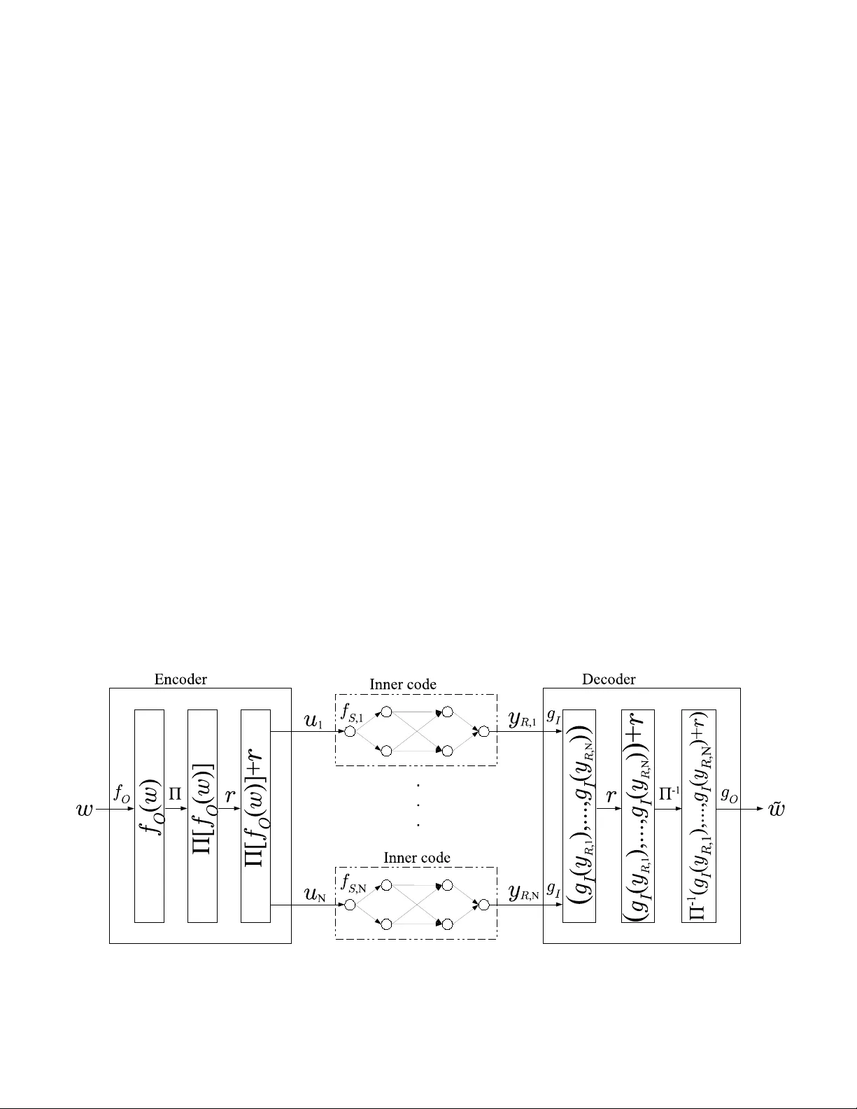
Lo w-Comple xity Near -Optimal Codes for Gaussian Relay N etw orks Theodo ros K. Dikaliotis 1 , Hongyi Y ao 1 , A. Salman A vestimeh r 2 , Sidharth Jag gi 3 , T rac ey Ho 1 1 California Institute of T echnolo gy 2 Cornell Univ e rsity 3 Chinese Un iv er sity of Hon g K ong 1 { tdikal, tho } @caltech .edu 1 yaoho ngyi03 @gmail.com 2 av e stimehr@ece.cor nell.edu 3 jaggi@ie.cuhk .edu.h k Abstract W e consid er the problem of information fl o w ov er Gaussian relay networks. Similar to the recent work by A v estimehr et al. [1], we propose network codes that achie ve up to a constant gap from the capacity of such networks. Howe ver , our proposed codes are also comp utationally tractable. Our main techniqu e is to use the cod es of A vestimehr et al. as inner codes in a concatenated coding scheme. I . I N T R O D U C T I O N The recent work of [1] para llels the classical network coding results [2] for wireless network s. That is, it introduc es a quantize-m ap-and -forward schem e that achie ves all rates up to a constant ga p to th e cap acity of Gau ssian relay networks, where th is con stant dep ends only o n the netw ork size, and varies linear ly with it. Howe ver the comp utational complexity of encodin g a nd decoding for the co des o f [1 ] g rows exponentially in the block -length. In this work, we aim to construct low co mplexity cod ing schemes that achieve to within a constant g ap of the cap acity of Gaussian relay networks. The simp lest Gaussian network th at has been well inv e stigated in the coding literatur e is th e point- to-poin t Add iti ve White Gaussian Noise ( A WGN) cha nnel. There have b een a v a riety of capac ity achieving co des developed for such c hannels (see e.g. , [3], [4], [5], [6] and referen ces therein) . There have also b een se veral recent efforts (fo r instan ce [7] an d [8]) to extend the resu lt of [1] and build low comp lexity relaying strategies that achieve up to a constant gap f rom the capacity of Gaussian relay n etworks. Howe ver th e decod ing complexity of the prop osed codes is still expo nential in the block-len gth. Th is is be cause th ese strategies are based o n la ttice codes, in wh ich d ecoding proceed s via n earest neighb our sear ch, which in g eneral is c omputatio nally intr actable. In this pap er , we build a coding sche me th at h as compu tational complexity that is p olynom ial in the block-len gth 1 and achieves ra tes up to a constant gap to th e cap acity of Gau ssian relay networks. More specifically , we build a Forney-typ e [ 9] two-layered concatenated code con struction fo r Ga ussian relay networks. As our inn er cod es we use improved versions of the in ner cod e in [1], which can be d ecoded with prob ability of erro r d roppin g exponentially fast in the in ner code block -length. As ou r outer codes we use polar codes [10], which are p rovably cap acity 1 The computa tional complexi ty of all existing code s, such as in [1], also grow e xponentiall y in netw ork paramete rs, namely the number of nodes |N | . In fac t, the code s proposed in this wo rk hav e the same property . Howe ver , for our purposes we con sider the net work size to be fixed and small. achieving (asy mptotically in their block -lengths) for th e Binary Symmetr ic Chan nel, and have comp utational co mplexity that is n ear-linear in their block-len gths. I I . M O D E L W e consider an ad ditiv e white Gaussian noise (A WGN) r elay network G = ( N , E ) , where N den otes the set of n odes and E the set o f edges b etween no des. W ithin th e n etwork there is a source S ∈ N and a sink no de 2 R ∈ N where the so urce has a set of messages it tries to co n vey to the sink. For ev ery node i ∈ N in th e network there is th e set I i = { j ∈ N : ( j, i ) ∈ E } ⊆ N of nodes that have ed ges incoming to n ode i . All nodes have a single rece iving and tra nsmitting an tenna and th e r eceiv ed signal y i,t at node i at time t is given b y y i,t = X j ∈I i h j i x j,t + z i,t (1) where x j,t ∈ C the signal transmitted from no de j at time t an d h j i ∈ C is the ch annel g ain associated with the ed ge conn ecting nodes j and i . The receiver n oise, z i,t , is mo deled as a complex Gau ssian ra ndom variable C N (0 , 1) , with i.i.d . distribution across time. Further we assume tha t there is an average tr ansmit power constraint equal to 1 a t each n ode in the network. W ithou t loss of generality we assume that network G has a layered structure, i.e. , all paths from the source to the destination have equal length. Th e numb er of la yers in G is deno ted by L G , an d th e source S r esides at layer 1 whe reas the sink R is a t layer L G . As in Section VI-B of [1] the re sults o f this pap er ca n be extended to the general case by expand ing the n etwork over tim e since the time -expanded network is lay ered. I I I . T R A N S M I S S I O N S T R AT E G Y A N D M A I N R E S U LT Fig. 1. System dia gram of our concat enated code desig n. 2 Just as in wired network coding, this result ex tends directly to the case of multiple sinks – to ease notati onal burde n we focus on the case of a single sink. Our sour ce enco der operates at two levels, respectively the outer co de level and the in ner co de lev e l. The o uter co de we u se is a polar code [11] (along with a ran dom per mutation of bits p assed from the outer code to the encod ers for the inne r co de – this p ermutation is used for tech nical r easons th at sh all b e described later). The inn er c ode is a random cod e similar to the inn er code u sed in [1]. The r elay n odes use “quan tize-map-an d-forward” as in [1] over a short block-leng th ( i.e. , the b lock-leng th of the inner code). Finally the r eceiver decodes the inner coding operations, in verts the ra ndom permutation in serted by the source encoder, and finally decode s the correspo nding outer polar code. The reason for using a two-layered concatenated code is to achieve b oth lo w encodin g and decod ing com plexity , and a decodin g erro r prob ability that de cays almo st exponentially fast with the block-leng th. In particular, as we describe in Section IV, our inne r co des have a deco ding alg orithm that is based on exhaustive search . T o en sure our inner codes’ decodin g comp lexity is tractable we set the bloc k-length of the inner codes to be a “ relatively small” fixed value. As a result, the decodin g e rror proba bility for o ur inner codes is also fixed. T o c ircumvent this, we then add an outer co de on top of the inner code. Mor e specifically , w e use a po lar code as an ou ter code, since polar cod es hav e m any desirable proper ties – in particular, they provably have encod ing an d d ecoding comp lexities tha t are near lin ear in the b lock-leng th, are asympto tically capacity achieving, a nd also hav e pr obability of er ror that decays nearly exponen tially in the blo ck-length [11]. One technical cha llenge arises. Polar codes are capab le of correcting indepen dent bit flips, but are not guaran teed to work against bursts of consecu tiv e bit flips. It is to “sprea d o ut” the possibly correlated bit-flip s that would occur if one or several inner co des d ecode inc orrectly that we intr oduce the random p ermutation mention ed above to the outpu t of the source en coder’ s outer p olar cod e. T his ran dom perm utation is based on pu blic rand omness, an d henc e is a vailable to both the source encoder, and the sink decod er (which can therefo re in vert it). The system diagram of o ur coding scheme is shown in Figure 1. W e now describe the details o f the encodin g, re laying, and d ecoding op erations used by the so urce, relay nodes and the sink. Also, the source outer code e ncoder XORs a rand om string (denoted r , and kn own in ad vance to all parties via p ublic ran domn ess) to its outp ut a fter permu ting the bits o f the polar co de, but befo re passing th ese bits to the inner codes. This is to ensure indepen dence of the in puts to the inner cod es, so that concen tration results can be used. A. En coding at the Sou r ce and the Relays The overall c ommun ication scheme is over n time instants and has a rate of R = R O R I , where R O and R I are the rates for the o uter cod e, and each o f th e inn er code s, respec ti vely . The source takes a m essage w ∈ F 2 R O R I n of size R O R I n bits, and first applies the encodin g algorithm of th e p olar code f O : F 2 R O R I n → F 2 R I n creating a string f O ( w ) ∈ F 2 R I n of R I n b its. Once the vector f O ( w ) is for med a ra ndom per mutation Π is applied on all the bits of f O ( w ) gi v ing rise to Π [ f O ( w )] ∈ F 2 R I n . A random length- R I n bit-vector r is then XORed with Π [ f O ( w )] ∈ F 2 R I n . The d erived bit-vecto r Π [ f O ( w )] is divided in N = n ℓ , i.e. Π [ f O ( w )] = ( u 1 , . . . , u N ) , chunk s of size R I ℓ bits, i. e. u k ∈ F 2 R I ℓ for 1 ≤ k ≤ N . Each one of the bit-vectors u k is conveyed throu gh the network ind epende ntly using a sepa rate random inner co de o f r ate R I and block-len gth ℓ in troduce d in [1]. More spe cifically , all no des in the network operate over blocks of length ℓ . The source rando mly maps ea ch inner code symbol u k ∈ { 1 , . . . , 2 R I ℓ } to a tran smitted vector of length ℓ with compon ents distributed i.i.d. from C N (0 , 1) . Th at is, for each 1 ≤ k ≤ N the rand om inn er codes operate as F S , k :  1 , 2 , . . . , 2 R I ℓ  → C ℓ , where realization s of F S , k are denoted f S , k . For ea ch 1 ≤ k ≤ N , each relay no de i ∈ G roun ds the re al and imaginary p art of each compo nent of its received vector y i,k ∈ C ℓ to the closest integer to form the length- ℓ vector ( [ y i,k ] ). It then rand omly maps [ y i,k ] it to a transmit vector of length ℓ with compo nents distributed i.i.d. f rom C N (0 , 1) . For each 1 ≤ k ≤ N the mapping s at relay i ∈ N ar e denoted by F i,k :  A ℓ i , A ℓ i  → C ℓ , with f i,k denoting a specific realization of F i,k . Here A i = {− s i , . . . , s i } is the set of integers from − s i to s i , wh ere s i is a co de design parame ter be specified later . If the inco ming signal at a relay n ode h as a comp onent such that its rea l or imag inary p art is larger than s i in magn itude then an erro r is declared . Finally , the sink R rece i ves y R ,k ∈ C ℓ associated w ith inner code sym bol u k . B. Deco ding At the end of the tr ansmission sch eme, sink R receives y R ∈ C n , wh ich consists of N chunk s of length ℓ , i.e. y R = ( y R , 1 , . . . , y R ,N ) where y R ,k ∈ C ℓ . For each chunk y i,k , 1 ≤ k ≤ N , the sink R th en a pplies th e d ecoding alg orithm g I : C ℓ → 2 R I ℓ of the correspon ding inner co de ( to b e descr ibed in Section IV). The sink then o btains ˆ u k , a po ssibly n oisy version o f the correspond ing inner code length- ℓ b it-vector u k that was tra nsmitted d uring the k th application of the inner co de. After decodin g all chunk s, it then XORs out the random bit-string r added as part of the encodin g procedu re and then the inv e rse of the permutatio n applied by the source enc oder is ap plied, i. e. Π − 1 [( g I ( y R , 1 ) , . . . , g I ( y R ,N ))] . Finally , th e sink utilizes th e polar code decoder in order to prod uce the e stimate for the source message, i.e. ˜ w = g O  Π − 1 [( g I ( y R , 1 ) , . . . , g I ( y R ,N ))]  . An error is de clared if w 6 = ˜ w . C. Ma in Re sult As in [1] we defin e ¯ C to be the cut-set u pper b ound on th e cap acity C of a g eneral Gaussian r elay n etwork, i.e. , C ≤ ¯ C ≡ max p ( { x j } j ∈N ) min Ω ∈ Λ G I ( Y Ω c ; X Ω | X Ω c ) where Λ G = { Ω : S ∈ Ω , R ∈ Ω c } d enotes the set o f all sou rce-sink cu ts. W e n ow state o ur main r esult. Theorem 1. F or a ny Gaussian r elay network, the codin g strate gy described above achieves all rates within (16 |N | + 2 ) bits fr om the cut-set upper bou nd ¯ C . This code ha s encod ing co mplexity of O( n lo g n + n 2 ¯ C l og ¯ C ) , decod ing complexity o f O( n log n + n 2 ( ¯ C +13 |N | ) l og 2 ¯ C ) , and a pr oba bility of err or decayin g as O(2 − n − 1 / 4 ) . The rest of th e paper is devoted to proving this Theorem . First we give the deco ding algorithm of the in ner code that is based on exhau sti vely sear ching “all po ssible” n oise pattern s in the network. Th en we contin ue specify ing desirable parameter for our code. I V . D E C O D I N G O F T H E I N N E R C O D E In [1] they p roved that by usin g their in ner code–th at is very sim ilar to ou r in ner cod e–the m utual inform ation b etween the source me ssage and wh at sink R re ceiv e s is with in a constant gap from the capacity . Therefo re by apply ing an outer channel code, any rate up to the mutu al in formation a nd con sequently rates within a co nstant gap from the capacity are achievable. In this work , despite ou r inner cod e is very similar to th at in [1] we do not u se a mutual infor mation type of argument but we instead d evise an exhaustively search type of a de coding algorithm f or the inn er c ode. More specifically once the sink R g ets the recei ved ℓ –tuple vector ( y 1 , . . . , y ℓ ) it rounds ev ery compo nent, i.e. ([ y 1 ] , . . . , [ y ℓ ]) and then it exhaustiv ely tries all po ssible messages u ∈ { 1 , . . . , 2 R I ℓ } an d all highly p robable no ise pattern s that g iv e d istinct outputs to fin d which was th e source me ssage that co uld have c reated the re ceiv e d signal. A d ecoding error is declared if th ere are m ore than one so urce messages u tha t could have given th e received signal or if there are no messages at all. Since the no ise at each nod e is a contin uous ra ndom variable ther e is an infinite n umber of possible noises that can occur ev e n at a sing le time in stance. Ther efore it is impossible to exhaustively search all possible noises tha t hap pened dur ing all ℓ time steps of the inner c ode block -length. Due to the fact though that every re lay nod e round s its received sig nal to the clo sest integer only a countable numbe r of n oise patterns would give different receiv e d sign als. Moreover we will show b elow that o ut of these in finite but coun table many noises there is a finite set of no ises th at happ en with high pro bability and the prob ability that there a noise p attern hap pens and does n ot be long to th at set is very sma ll. A. Qu antized no ise In the following we will formalize all the above and we will start b y g i ving the d efinition o f quantized noise. Definition 1. The quantized noise q i,t for node i ∈ N at time t is defined a s q i,t = [ y i,t ] −   X j ∈G i h j i x j,t   (2) wher e [ w ] is the r oun ding of the real a nd imaginary part of the complex nu mber w ∈ C to the closest integ e r . Since y i,t = P j ∈G i h j i x j,t + z i,t it is shown in Ap pendix B th at the quantized n oise q i,t can be written in th e fo rm q i,t = [ z i,t ] + R i,t (3) where R i,t can take any of the 9 v alu es R i,t = a i,t + b i,t i with i 2 = − 1 , a i,t , b i,t ∈ { − 1 , 0 , 1 } and z i,t is distributed as C N (0 , 1 ) for all t ∈ { 1 , . . . , ℓ } . Equatio n (2) g iv e s th at the quantized version of the received signal is g iv e n b y the quantiza tion o f th e transmitted signal plus the quantized noise. Theref ore o ut o f all the countab ly many quantized noise ℓ -tuples ( q i, 1 , . . . , q i,ℓ ) we want to find a finite set Q ℓ called the “can didate qu antized noise set” wh ere the most p robab le quantized n oise ℓ –tu ples are co ntained. W e will use this set Q ℓ for ou r exha ustiv e search alg orithm. B. Can didate q uantized n oise set One co uld po ssible ch oose the candidate quantized noise set Q ℓ to b e the typical set for ran dom variable q i,t as defined in Chapter 3 o f [1 2]. T he diffi culty with this approach is that we do n ot know th e distrib ution of q i,t , since th e d istribution of R i,t is un known and moreover ran dom variables z i,t and R i,t are cor related. On the other h and we know the distribution o f random variables z i,t and we will define set Z ℓ to be: Definition 2. The set o f Z ℓ is th e set o f those ℓ –tuples ( [ z 1 ] , . . . , [ z ℓ ]) ∈ Z ℓ such that p ([ z 1 ] , . . . , [ z ℓ ]) ≥ 2 − 9 ℓ , wher e p ([ z 1 ] , . . . , [ z ℓ ]) is the pr o bability of the ℓ –tuple a nd z i ar e i.d.d. C N (0 , 1) rando m variables. From the de finition above 3 it is clear th at set Z ℓ has at most 2 9 ℓ elements, i.e. | Z ℓ | ≤ 2 9 ℓ . In A ppendix D it is proved that the pro bability of som e ℓ –tuple ([ z 1 ] , . . . , [ z ℓ ]) ( z i are i.i.d. C N (0 , 1) random variables) drawn random ly from C N (0 , 1) to be outside of Z ℓ drops as 2 − 2 ℓ . Moreover in App endix C a rand om proced ure that is based on th e “Cou pon Collec tor Pr oblem” is prop osed on how to find all the elem ents in Z ℓ with probab ility o f failure ( missing some elements of Z ℓ ) dropp ing as fast as 2 − ℓ . The ra ndom variable R i,t defined in equ ation (3) takes 9 p ossible values. Ther efore there are 9 ℓ possible ℓ – tuples ( R i, 1 , . . . , R i,ℓ ) and the set tha t c ontains all 9 ℓ such ℓ –tuples is called set R ℓ . No w we ar e ready to give the definition of the candidate q uantized noise set Q ℓ : Definition 3. The candida te qua ntized noise set Q ℓ is th e set o f all ℓ tup les of qu antized n oise such that Q ℓ = { z i + r j : ∀ z i ∈ Z ℓ and r j ∈ R ℓ } denoting the su m of all Z ℓ ℓ –tuples with all possible R ℓ ℓ –tuples. From the defin ition above along with Append ix C since we considers all po ssible ℓ –tup les of R i,t , no matter what the exact distribution of R i,t is, the probab ility that a quan tized noise ℓ – tuple Q = ( q i, 1 , . . . , q i,ℓ ) rando mly chosen will be outside Q ℓ will b e given by P ( Q / ∈ Q ℓ ) ≤ 2 − 2 ℓ . (4) It is easy to see that the size of set Q ℓ is upper b ound ed by | Q ℓ | ≤ 9 ℓ | Z ℓ | ≤ 9 ℓ 2 9 ℓ < 2 13 ℓ . From n ow on we will assume that if a q uantized ℓ – tuple that “ occurs” in any node in the n etwork is o utside Q ℓ then this is declare d as an erro r and du e to (4) this error ha ppens with p robability less than 2 − 2 ℓ . C. P r obab ility of indistinguisha bility As we discussed be fore once the sink R round s its rece iv ed signal ℓ –tuple vector ([ y 1 ] , . . . , [ y ℓ ]) it exha ustiv ely tries all possible messages u ∈ { 1 , . . . , 2 R I ℓ } and all quantized noise tu ples in Q ℓ to find which was the sour ce message that could have cr eated the received sign al. An erro r in the decodin g o f th e inner co de o ccurs if a noise pattern outside of Q ℓ occurs in some no de i ∈ N . Then the de coding of the inner code fails and th is ha ppens with pro bability at most |N | 2 − ℓ accordin g to (4) and the union bou nd over all n odes. Mo reover if the n oise patterns in all no des happ en inside Q ℓ then the inner code fails 3 The entrop y of the random varia ble [ z ] where z is distrib uted as C N (0 , 1) is around 4 . 4 and therefore the typica l set as defined in [12] will contai n all ℓ –tuples ha ving probabilit y 2 − (4 . 4 ± ǫ ) ℓ . Theref ore set Z ℓ contai ns the typic al set for ǫ ≤ 4 . 6 . if there are more th an one messages u that would have given rise to the same received signal a nd in the following we will analyze this probab ility P ( u → u ′ ) . Assume th at th e sou rce no de S sends message u and the qua ntized noise realization q G under message u at all th e no des in the network is q G = a . Th en P ( u → u ′ ) is the prob ability th at th ere is anothe r me ssage u ′ ( u ′ 6 = u ) and som e noise realization q ′ G = b under m essage u ′ (the two noise realization s are not nec essarily different) so that th e sin k R cannot d istinguish wh ether message u or u ′ was sent. Similar to [1] equatio n (70) we have P ( u → u ′ | q G = a , q G = b ) = X Ω ∈ Λ G P Ω , a , b (5) where Ω is any cut in th e network and P Ω , a , b is d efined to be th e prob ability tha t nodes in Ω can distinguish between sourc e messages u an d u ′ under the no ise realization a and b resp ectiv e ly while nodes in Ω c cannot distingu ish u and u ′ . It is proved in Append ix E th at this probab ility is upp er b ound ed by P Ω , a , b ≤ 2 − ℓ ( ¯ C − 3 |N | ) . (6) Assume th at th e sou rce no de S sends message u and th e q uantized no ise realization in every nod e in th e n etwork is a , then the proba bility that there is an other m essage u ′ or quantized n oise ℓ –tup le in Q ℓ that will confuse th e receiver is given by P ( u → u ′ ) ≤ P Ω , a , b 2 R I ℓ | Q ℓ | |N | ( 6 ) ≤ 2 − ℓ ( ¯ C − 3 |N | ) 2 R I ℓ | Q ℓ | |N | ≤ 2 − ℓ ( ¯ C − 3 |N | ) 2 R I ℓ 2 13 ℓ |N | ≡ 2 − ℓ ( ¯ C − 16 |N |− R I ) Therefo re b y setting the ra te of th e inner co de R I = ¯ C − 16 |N | − 1 (7) the proba bility that two messages u and u ′ will be indistinguishab le at the r eceiv er R decays as P ( u → u ′ ) ≤ 2 − ℓ (8) Finally at each node we h av e some map pings F i :  A ℓ i , A ℓ i  → C ℓ where A i is the set of integers {− s i , . . . , s i } so that th e probab ility o f a incom ing signal h aving a co mponen t o utside of A i to be very small. Spe cifically for e very nod e i ∈ N th ere is a set of signals that give th e ma ximum a bsolute value M i for the re ceiv e d real or imaginar y part, i.e. M i = max j ∈G i ,t          Re   X j ∈G i h j i x j,t         ,       Im   X j ∈G i h j i x j,t            then s i = M i + δ i where δ i > 0 c orrespon ds to th e smallest slack nece ssary to make sure that the rece i ved signal (tr ansmitted signal + no ise) is less in absolute value th an s i with probab ility at mo st 2 − 2 ℓ . If the rec eiv e d sign al has a real or imag inary part tha t its absolute value exceeds s i then th e noise should have a real or im aginary part with ab solute value larger than δ , i.e. P ( z ≥ δ i ) ( ∗ ) ≤ Exp  − δ 2 i 2  ≤ 2 − 2 ℓ ⇒ δ i = ⌈ √ ℓ 2 ln 2 ⌉ . where inequality ( ∗ ) is derived by inequality (7 . 1 . 13 ) at page 298 of [13]. D. Pr o bability of err o r for the in ner code Now we ar e r eady to analy ze the overall pro bability of error f or the inn er cod e. The inner code fails if on e o f the following four events hap pen: 1) Some node i ∈ N in the network rece i ved a signa l that its com ponent has a re al or an ima ginary par t with ab solute value larger than s i . According to the analysis above this event happ ens w ith probab ility less than 2 − 2 ℓ |N | ≤ 2 − ℓ for large enoug h ℓ ( ℓ ≥ log 2 ( |N | )) . 2) The ran dom procedure th at finds all the elements o f set Q ℓ failed. According to Appendix D this happens with probability less than 2 − ℓ . 3) The quantized noise in some no de i ∈ N in the network is o utside of set Q ℓ and acc ording to ( 4) this happ ens with probab ility less than 2 − 2 ℓ |N | ≤ 2 − ℓ for large enoug h ℓ ( ℓ ≥ log 2 ( |N | )) . 4) If th e exhaustive search decodin g pro cedure fails b ecause there are more than o ne q uantized noises ℓ –tuples or messages that give the same signal to the receiv er and accord ing to (8) this happen s with prob ability less than 2 − ℓ and therefore the overall pr obability o f e rror P I for the in ner code is up per bo unded b y P I ≤ 4 2 − ℓ (9) for ℓ > log 2 ( |N | ) . E. Comp lexity of the inner co de In order to imp lement the inner code one have to fin d set Q ℓ . This is d one by finding set Z ℓ and the rand om approach based on the “Coup on’ s Collector Pro blem” to create set Z ℓ requires O( ℓ 2 9 ℓ ) order of steps. The mo st “expensive” o peration thoug h for the inne r co des is the exhau sti ve decodin g tha t search over all elem ents in Q ℓ ( Q ℓ ≤ 2 13 ℓ ) over all no des in the n etwork |N | and over all m essages an d th erefore incurring an d overall com plexity 2 R I ℓ 2 R I +13 |N | ℓ = 2 ( R I +13 |N | ) ℓ ≈ 2 ( ¯ C +13 |N | ) ℓ . V . C O M P L E X I T Y A N D E R R O R A N A LY S I S O F T H E C O D E W e now sp ecify the value o f th e p arameter ℓ ( which was left open thus far). For reasons that shall be clear in equation (11) for the re st o f the p aper we ch oose ℓ so that h (2 P I ) ≤ 1 ¯ C (10) where h ( x ) = − x log 2 x − (1 − x ) log 2 (1 − x ) is the entro py f unction. The exact value for the prob ability of error fo r the inner cod e is not known but we can b e pessimistic and take its largest value P I ≤ 4 2 − ℓ giv en by 9. One p ossible value for ℓ that satisfies in equality ( 10 ) as it is p roved in Appendix F is ℓ = 3 + ⌈ lo g 2 ¯ C ⌉ and that is the value we will set the blo ck length of the inn er c ode to get. A. Pr o bability of err o r For ea ch inner co de th at d ecodes its chunk inco rrectly , in the worst c ase th ere is a burst of R I ℓ erroneo us bits that are p assed to the sink’ s the p olar code d ecoder . The p urpo se of the outer polar code is to co rrect these bit flips. Ou t of the N = n ℓ input length- ℓ bit-vectors to the outer code on average o nly n ℓ P I are decoded erroneo usly ( again, this numb er is co ncentrate d ar ound the expected value with high p robab ility). This correspond s to n ℓ P I R I ℓ = n P I R I bit flips. Sin ce each inn er code ch unk has indepen dent inpu ts (due to the XORing ope ration d escribed in the encod er) and is decoded independ ently we ca n apply the Chernoff bound and prove ( Append ix G) that the p robability of h aving more than twice th e expected nu mber of bit flips drops at least as Ex p ( − 0 . 15 n ¯ C log 2 ¯ C ) . The rate of the p olar co de is chosen R O = 1 − h (2 P I ) can corr ect bit flips th at are injected in ou r ch annel with probab ility only P I . Therefo re when less than twice the expected numb er of bit flips happen then the polar c ode fails with prob ability 2 − ( nR I ) β for any β < 1 / 2 as proved in [11] ( the b lock-len gth of the polar code is nR I ). Therefor e the p robability of error of the overall code is d ominated by th e p robability of er ror fo r th e po lar c ode is o f the o rder O (2 − n 1 / 4 ) f or β = 1 / 4 . B. Achievable rate The achiev able rate is R = R O R I or R ≥ ¯ C − 1 6 |N | − 2 (1 1) since R I = ¯ C − 16 |N | − 1 and R O ≥ 1 − 1 ¯ C due to (1 0). C. E ncodin g d ecoding co mplexity The encoding and decoding co mplexity of our codes is the following: • The encoding c omplexity for the outer polar code i s O( n log n ) w hile the encoding complexity per inner code is O(2 ¯ C log ¯ C ) so the overall enc oding complexity is O( n lo g n + n 2 ¯ C log ¯ C ) • The decod ing comp lexity of the polar co de is O( n log n ) whereas th e decoding co mplexity per inner code is O(2 ( ¯ C +13 |N | ) log ¯ C ) so th e overall en coding co mplexity is O( n log n + n 2 ( ¯ C +13 |N | ) l og 2 ¯ C ) . R E F E R E N C E S [1] A. S. A vesti mehr , S. N. Diggavi, and D. N. C. Tse, “W ireless netw ork information flo w: A deterministic approac h, ” to appea r in IEEE T ransact ions of Informatio n Theory . [Online]. A v ailable : http://arxi v .org/PS cache /arxi v/pdf/0906/0906.5394v6.pdf [2] R. Ahlswede, N. Cai, S.-Y . Li, and R. Y eung, “Network information flow , ” IEEE T ransaction s on Information Theory , vol. 46, no. 4, pp. 1204–1216, July 2000. [3] U. Erez and R. Zamir , “ Achie ving 1 2 log(1 + SNR ) on the A WGN channel with latti ce encodi ng and decoding, ” IE EE T ransacti ons on Information Theory , v ol. 50, no. 10, 2004. [4] A. R. Barron and A. Joseph, “T o ward fast reliable communicat ion at rates near capac ity with gaussian noise , ” in P r oc. of the IE EE Information Theory W orkshop , Austin, T ex as, 2010. [5] N. Sommer , M. Feder , and O. Shalvi, “Lo w density latti ce codes, ” in Proc . of the IEEE Informat ion Theory W orkshop , Seattle, W ashington , 2006. [6] U. W achsmann, R. F . H. Fischer , and J. B. Huber , “Mul tilev el codes: Theoretical concepts and practica l design rules, ” IEE E T ransactions on Information Theory , v ol. 45, no. 5, 1999. [7] W . Nam, S. -Y . Chung, and Y . H. Lee, “Nested lattice codes for gaussian relay networks with interfere nce, ” s ubmitte d to IEE E T ransactions on Information Theory . [8] A. ¨ Ozg ¨ ur and S. Diggavi , “ Approximat ely achie ving gaussian relay network capacity with lat tice codes, ” in Pro c. of the IEEE Internatio nal Symposium on Informat ion Theory , Austin, T e xas, 2010. [9] G. D. Forne y , Concate nated Codes . Cambridge , MA: MIT Press, 1966. [10] E. Arikan, “Channel polarizat ion: A method for construct ing capacity-ac hieving codes for symmetric binary-inpu t memoryle ss channels, ” in Pro c. of the IEEE International Symposium on Informat ion Theory , T oronto, Canada, 2008. [11] E. Arikan and E. T elata r, “On the rate of channel polariza tion, ” in Pr oc. of the IEEE Informat ion Theory W orkshop , Seoul, Korea, 2009. [12] T . Cov er and J. T homas, E lements of Information Theory . W iley , 2006. [13] M. Abramo witz and I. A. Ste gun, Handbook of Mathemati cal Functions with F ormul as, Gra phs, and Mathemat ical T ables , 9th ed. Ne w Y ork: Dov er, 1964. [14] M. Mitzenmac her and E. Upf al, Pr obability and Computing: Randomized Algorit hms and Pro babilist ic Analysis . Cambridge Univ ersity Press, 2005. A P P E N D I X A P R O O F O F L E M M A 1 Consider the SVD d ecompo sition of H : H = UΣV † , with singu lar values σ 1 , . . . , σ min( n,m ) . For every vector f ∈ C n × 1 where || f || ∞ ≤ √ 2 th en || f || ∞ ≤ √ 2 n an d therefore P  ∀ 1 ≤ t ≤ ℓ :       H [ ˜ x 1 ,t , . . . , ˜ x m,t ] T + r t       ∞ ≤ √ 2  ≤ P  ∀ 1 ≤ t ≤ ℓ :       H [ ˜ x 1 ,t , . . . , ˜ x m,t ] T + r t       2 ≤ √ 2 n  = P  ∀ 1 ≤ t ≤ ℓ :       U  ΣV † [ ˜ x 1 ,t , . . . , ˜ x m,t ] T + U † r t        2 ≤ √ 2 n  ( a ) = P  ∀ 1 ≤ t ≤ ℓ :       ΣV † [ ˜ x 1 ,t , . . . , ˜ x m,t ] T + U † r t       2 ≤ √ 2 n  ( b ) = P  ∀ 1 ≤ j ≤ ℓ :       Σ [ ˜ x 1 ,t , . . . , ˜ x m,t ] T + ˜ r t       2 ≤ √ 2 n  = P   ∀ 1 ≤ t ≤ ℓ : min( n,m ) X i =1 ( σ i ˜ x i,t + ˜ r i,t ) 2 + n X i =min( n,m )+1 ˜ r 2 i,t ≤ 2 n   = P   ∀ 1 ≤ t ≤ ℓ : min( n,m ) X i =1 ( σ i ˜ x i,t + ˜ r i,t ) 2 ≤ 2 n − n X i =min( n,m )+1 ˜ r 2 i,t   = ℓ Y t =1 P   min( n,m ) X i =1 ( σ i ˜ x i,t + ˜ r i,t ) 2 ≤ 2 n − n X i =min( n,m )+1 ˜ r 2 i,t   (12) where equality ( a ) holds due to the fact that unitary matrices preserve the norm– 2 o f a vector , ( b ) holds since V † [ ˜ x i, 1 , . . . , ˜ x i,ℓ ] T have th e same distribution with [ ˜ x i, 1 , . . . , ˜ x i,ℓ ] T and ˜ r = U † r . W e will den ote by P j the f ollowing probab ility P j = P   min( n,m ) X i =1 ( σ i ˜ x i,t + ˜ r i,t ) 2 ≤ ω   (13) where ω = 2 n − n X i =min( n,m )+1 ˜ r 2 i,t and therefore P j = P   min( n,m ) X i =1 ( σ i ˜ x i,t + ˜ r i,t ) 2 ≤ ω   = P   − k min( n,m ) X i =1 ( σ i ˜ x i,t + ˜ r i,t ) 2 ≥ − k ω   ∀ k > 0 = P   Exp   − k min( n,m ) X i =1 ( σ i ˜ x i,t + ˜ r i,t ) 2   ≥ Exp [ − k ω ]   ( c ) ≤ E    Exp   − k min( n,m ) X i =1 ( σ i ˜ x i,t + ˜ r i,t ) 2      Exp [ k ω ] ( d ) = Exp [ k ω ] min( n,m ) Y i =1 E n Exp h − k ( σ i ˜ x i,t + ˜ r i,t ) 2 io = Exp [ k ω ] min( n,m ) Y i =1 1 √ 2 π σ 2 Z + ∞ −∞ Exp  − k ( σ i y + ˜ r i,t ) 2  Exp  − y 2 2 σ 2  dy = Exp [ k ω ] min( n,m ) Y i =1 Exp  − ˜ r 2 i,j t 1+2 σ 2 i σ 2 t  p 1 + 2 σ 2 i σ 2 t , (14) where ( c ) is the Markov inequality and ( d ) holds since ˜ x i,t are indepen dent fo r different t . From eq uation (14) f or k = 1 2 σ 2 we get P j ≤ Ex p h ω 2 σ 2 i min( n,m ) Y i =1 Exp  − ˜ r 2 i,t 2 σ 2 (1+ σ 2 i )  p 1 + σ 2 i = Ex p   1 2 σ 2   ω − min( n,m ) X i =1 ˜ r 2 i,t 1 + σ 2 i     Exp   − 1 2 min( n,m ) X i =1 ln(1 + σ 2 i )   and by su bstituting ω with its value ω = 2 n − n X i =min( n,m )+1 ˜ r 2 i,t along with the equation ab ove we g et P j ≤ Ex p   1 2 σ 2   2 n − n X i =min( n,m )+1 ˜ r 2 i,t − min( n,m ) X i =1 ˜ r 2 i,t 1 + σ 2 i     Exp   − 1 2 min( n,m ) X i =1 ln(1 + σ 2 i )   ≤ Ex p  1 2 σ 2 (2 n )  Exp   − 1 2 min( n,m ) X i =1 ln(1 + σ 2 i )   ≤ Ex p   − 1 2   min( n,m ) X i =1 ln(1 + σ 2 i ) − 2 n σ 2     and combinin g th e inequality above with (12) we get P  ∀ 1 ≤ j ≤ ℓ :       H [ ˜ x 1 ,j , . . . , ˜ x m,j ] T + r j       ∞ ≤ √ 2  ≤ Exp   − ℓ 2   min( n,m ) X i =1 ln(1 + σ 2 i ) − 2 n σ 2     ≤ 2 − h ℓ 2  P min( n,m ) i =1 ln(1+ σ 2 i ) − 2 n σ 2 i log 2 e ≤ 2 − ℓ 2  P min( n,m ) i =1 log 2 (1+ σ 2 i ) − 2 n σ 2 log 2 e  and since, 1 2 P min( m,n ) i =1 log 2 (1 + σ 2 i ) = 1 2 log 2 det ( I n + H H † ) = I ( x ; H x + z ) , for x , z that are d istributed as C N ( 0 , I m ) and C N ( 0 , I n ) r espectrively we get P  ∀ 1 ≤ j ≤ ℓ :       H [ ˜ x 1 ,j , . . . , ˜ x m,j ] T + r j       ∞ ≤ √ 2  ≤ 2 − ℓ ( I ( x ; Hx + z ;) − n σ 2 log 2 e ) (15) A P P E N D I X B R O U N D I N G T O T H E C L O S E S T I N T E G E R T H E S U M O F T W O N U M B E R S W e d efine as [ x ] to be the nearest integer to some real number x and if z = a + b i ∈ C for a, b ∈ R a nd i 2 = − 1 then [ z ] = [ a ] + [ b ] i . Assume that h 1 = x 1 + y 1 and h 2 = x 2 + y 2 are two positive r eal num bers with x 1 , x 2 and y 1 , y 2 representin g the integer and decimal part of these number s. Th en if we wr ite [ h 1 + h 1 ] = [ h 1 ] + [ h 2 ] + L (a) The val ue of L for [ h 1 − h 2 ] = [ h 1 ] − [ h 2 ] + L (b) The valu e of L for [ h 1 − h 2 ] = [ h 1 ] − [ h 2 ] + L Fig. 2. The v alue of L for dif ferent regi ons of ( y 1 , y 2 ) and diffe rent operati ons (addition & subtraction) the different values o f L for d ifferent regions of ( y 1 , y 2 ) are given in Figure 2(a). Similarly if we take th e difference of h 1 and h 2 and we write [ h 1 + h 1 ] = [ h 1 ] + [ h 2 ] + L then the values of L fo r d ifferent regions of ( y 1 , y 2 ) a re shown in Figure 2(b). Therefo re in general for two complex nu mbers z 1 , z 2 ∈ C we have [ z 1 + z 2 ] = [ z 1 ] + [ z 2 ] + R where R can take one of the 9 values R = r 1 + r 2 i where r 1 , r 1 ∈ { − 1 , 0 , 1 } . A P P E N D I X C A R A N D O M A P P RO A C H T O FI N D A L L E L E M E N T S I N S E T Z ℓ The way to find all the elements in set Z ℓ = { z 1 , . . . , z | Z ℓ | } is based on the well known “Coupon Collector’ s Pr oblem” [14]. Let’ s assume that one cre ates r (the value of r will be specified later) ℓ –tuple s ([ z 1 ] , . . . , [ z ℓ ]) (where z i are i.i.d. rando m variables distributed as C N (0 , 1) ) and d enote as A r ℓ the set of all these r rand omly created ℓ –tup les. The probability that elem ent z i ∈ Z ℓ is not contained in the ra ndomly cre ated set A r ℓ is given by P ( z i / ∈ A r ℓ ) = (1 − p i ) r ≤ e − r p i where p i is the probability of e lement z i ∈ Z ℓ and since p i ≥ 2 − 9 ℓ ≡ Q the n P ( z i / ∈ A r ℓ ) ≤ e − r Q . Moreover fro m the d efinition of Q we g et that | Z ℓ | ≤ 1 Q and in gene ral the p robab ility that the re is an element in Z ℓ that is not contained in A r ℓ is P [ z i ∈ Z ℓ { z i / ∈ A r ℓ } ! ≤ X z i ∈ Z ℓ P ( z i / ∈ A r ℓ ) ≤ | Z ℓ | e − r Q ≡ 1 Q e − r Q and therefore if r = 10 9 1 Q ln  1 Q  we have tha t P [ z i ∈ Z ℓ { z i / ∈ A r ℓ } ! ≤ 1 Q e − 10 9 1 Q ln ( 1 Q ) Q = Q 1 9 and since Q = 2 − 9 ℓ P [ z i ∈ Z ℓ { z i / ∈ A r ℓ } ! ≤ 2 − ℓ and the n umber o f e lements in A r ℓ is 10 ℓ 2 9 ℓ ln 2 . A P P E N D I X D T H E P R O B A B I L I T Y T H A T A R A N D O M LY P I C K E D ℓ – T U P L E W I L L B E O U T S I D E S E T Z ℓ Assume that there is an ℓ –tup le Z = ([ z 1 ] , . . . , [ z ℓ ]) dr awn randomly where z ar e i.i.d. ra ndom variables from d istribution C N (0 , 1) then the prob ability that does not belong to Z ℓ is P [ Z / ∈ Z ℓ ] = P " ℓ Y i =1 p ([ z i ]) < 2 − 9 ℓ # = P " ℓ Y i =1 1 p ([ z i ]) > 2 9 ℓ # = P " ℓ Y i =1  1 p ([ z i ])  k > 2 9 kℓ # ∀ k > 0 ( a ) ≤ E  Q ℓ i =1  1 p ([ z i ])  k  2 9 kℓ ( b ) ≤ 2 − 9 kℓ ℓ Y i =1 E "  1 p ([ z i ])  k # = 2 − 9 kℓ  E  p − k ([ z ])  ℓ =  2 − 9 k E  p − k ([ z ])  ℓ ( c ) =  2 − 9 k E 2  p − k ([ z R ])  ℓ (16) where ( a ) is due to Ma rkov inequality and ( b ) is due to the indepen dence of the p ([ z i ]) for i ∈ { 1 , . . . , ℓ } . At equ ality ( c ) , z R is rando m variable distributed as N (0 , 1) and the eq uality holds since the r eal and the imag inary p art of a C N (0 , 1 ) random variable a re indepen dent N (0 , 1 ) random variables. If we de fine c i where i ∈ Z to b e c i = 1 √ 2 π Z i + 1 2 i − 1 2 e − x 2 2 dx then E  p k ([ z R ])  = ∞ X i = −∞ c 1 − k i = c 1 − k 0 + 2 ∞ X i =1 c 1 − k i . One ca n boun d c i by inequality (7 . 1 . 13) at page 2 98 o f [13]: c k ≤ Exp  − k 2 / 2  k 1 √ 2 π − r 2 9 π ! for k > 0 and appro ximating c 0 ≤ 0 . 5 . From the ab ove ineq ualities one can find that for k = 0 . 6 , E  p k ([ z R ])  ≤ 2 . 9 and ther efore from inequality (16) we get P [ Z / ∈ Z ℓ ] ≤ 2 . 9 2 2 9 · 0 . 6 ≤ (0 . 2) ℓ ≤ 2 − 2 ℓ . A P P E N D I X E A N A LY Z I N G P R O B A B I L I T Y P Ω , a , b The analysis is very similar to [1]. W e d efine P Ω , a , b = P  Nodes in Ω c an d istinguish between u , u ′ and nodes in Ω c cannot   q G = a , q ′ G = b  (17) where Ω is any cut in the network. W e define the following sets and ev ents: • L l (Ω) : The nodes that are in Ω and are at layer l . • R l (Ω) : The nodes that are in Ω c and are at laye r l . • L l (Ω) : Th e event that the nod es in L l (Ω) can distinguish between u an d u ′ . • R l (Ω) : Th e ev ent that the nodes in R l (Ω) can not d istinguish between u an d u ′ . The nodes in any set A can not disting uish between the message u and u ′ if the integer values of their received sign als a re identical, i.e. [ y A ( u )] = [ y A ( u ′ )] . Assume that the network is layered and there are L G layers in total (the sou rce S is at layer L = 1 and the receiv er R is at layer L G ). Therefo re equation (17) b ecomes P Ω , a , b = P  R l (Ω) , L l − 1 (Ω) , l = 2 , . . . , l D   q G = a , q ′ G = b  = L G Y l =2 P  R l (Ω) , L l − 1 (Ω)   R j (Ω) , L j − 1 (Ω) , j = 2 , . . . , l − 1 , q G = a , q ′ G = b  ≤ L G Y l =2 P  R l (Ω)   R j (Ω) , L j (Ω) , j = 2 , . . . , l − 1 , q G = a , q ′ G = b  ( ∗ ) = L G Y l =2 P  R l (Ω)   R l − 1 (Ω) , L l − 1 (Ω) , q G = a , q ′ G = b  = L G Y l =2 P  y R l (Ω) ( u )  =  y R l (Ω) ( u ′ )    R l − 1 (Ω) , L l − 1 (Ω) , q G = a , q ′ G = b  = L G Y l =2 P  ∀ 1 ≤ t ≤ ℓ :  H l x L l − 1 (Ω) ,t ( u )  + a R l (Ω) ,t =  H l x L l − 1 (Ω) ,t ( u ′ )  + b R l (Ω) ,t   R l − 1 (Ω) , L l − 1 (Ω) , q G = a , q ′ G = b  ( ∗∗ ) = L G Y l =2 P  ∀ 1 ≤ t ≤ ℓ :  H l x L l − 1 (Ω) ,t ( u ) + a R l (Ω) ,t  =  H l x L l − 1 (Ω) ,t ( u ′ ) + b R l (Ω) ,t    R l − 1 (Ω) , L l − 1 (Ω) , q G = a , q ′ G = b  where H l ∈ C | R l (Ω) |×| L l − 1 (Ω) | is the transf er matrix fr om the n odes in L l − 1 (Ω) to th e nod es in R l (Ω) . V ectors x L l − 1 (Ω) ,t ( u ) , x L l − 1 (Ω) ,t ( u ′ ) are the signals transmitted at time step t fr om nod es in L l − 1 (Ω) when the sou rce S ha s transmitted messages u and u ′ respectively whereas a R l (Ω) ,t , b R l (Ω) ,t are the no ise realization s for nodes in R l (Ω) at time t . Inequality ( ∗ ) ho lds due to the Mar kov structure o f the n etwork and ( ∗∗ ) the last equality hold s since the compo nents of a , b are in tegers. Note th at if A , B ∈ C m × 1 are co mplex vectors then [ A i ] = [ B i ] ∀ i ⇒ || A − B || ∞ ≤ √ 2 and therefore from th e previous equ ation we get P Ω , a , b ≤ L G Y l =2 P  ∀ 1 ≤ t ≤ ℓ :       H l  x L l − 1 (Ω) ,t ( u ) − x L l − 1 (Ω) ,t ( u ′ )  + ( a − b ) R l (Ω) ,t       ∞ ≤ √ 2 |R l − 1 (Ω) , L l − 1 (Ω) , z V = a , z ′ V = b  . W e ar e now extend ing Lemma 1 of [1] in th e following Lemma th at is p roved in Ap pendix A. Lemma 1. A ssume [ ˜ x i, 1 , . . . , ˜ x i,ℓ ] for i = 1 , . . . , m ar e vectors of length ℓ with elements chosen i.i.d. fr om C N (0 , σ 2 ) . Mor eover r j ∈ C n × 1 ar e a collection of vectors an d H ∈ C n × m is som e matrix then P  ∀ 1 ≤ j ≤ ℓ :       H [ ˜ x 1 ,j , . . . , ˜ x m,j ] T + r j       ∞ ≤ √ 2  ≤ 2 − ℓ ( I ( x ; Hx + z ) − n σ 2 log 2 e ) wher e x , z are d istrib uted as C N ( 0 , I m ) and C N ( 0 , I n ) r espec trively . Therefo re since  x L l − 1 (Ω) ,t ( u ) − x L l − 1 (Ω) ,t ( u ′ )  are Gaussian random variables distributed i.i.d. from C N (0 , 2) we have from ap plying Lemma 1 tha t P Ω , a , b ≤ l D Y l =2 2 − ℓ  I  x L l − 1 (Ω) ; y R l (Ω) | x R l − 1 (Ω)  − | R l (Ω) | 2 log 2 e  ≤ 2 − ℓ ( ¯ C iid −|V | ) (18) where ¯ C iid is d efined as Definition 4. W e defin e ¯ C iid = min Ω I ( x Ω ; y Ω c | x Ω c ) wher e x i , i ∈ V , ar e i.i.d . C N (0 , 1 ) rando m variab les an d Ω is any cut in the n etwork. Finally if we co mbine ( 18) with L emma 6 . 6 in [ 1] that gives ¯ C − ¯ C iid < 2 |N | we con clude that P Ω , a , b ≤ 2 − ℓ ( ¯ C − 3 |N | ) . A P P E N D I X F E V A L U A T I O N O F B L O C K - L E N G T H O F T H E I N N E R C O D E W e want to find a probability a value fo r x ≤ 1 2 such th at h ( x ) ≤ 1 ¯ C where h ( x ) = − x lo g 2 x − (1 − x ) log 2 (1 − x ) is th e entropy function . It requires simple algebra to p rove that h ( x ) < − 2 x log 2 x fo r x < 0 . 4 . Th erefor e if − 2 x log 2 x ≤ 1 ¯ C then h ( x ) < 1 ¯ C for x < 0 . 4 . For x = 1 ¯ C 2 we get − 2 ¯ C 2 log 2  1 ¯ C 2  < 1 ¯ C ⇒ 4 ¯ C log 2 ¯ C < 1 and that holds for ¯ C > 16 . From equation (7) we g et that ¯ C > 16 for the networks wh ere our co de construction would work o r else the rate of the inner code would be negativ e . So for the values of interest of ¯ C as long as we set 2 P I ≤ 9 82 − ℓ ≤ 1 ¯ C 2 ⇒ ℓ = 3 + ⌈ log 2 ¯ C ⌉ we ar e c ertain that h (2 P I ) ≤ 1 ¯ C for values of ¯ C that are of interest to us. A P P E N D I X G C H E R N O FF B O U N D For any random variable A and for every t ≥ 0 P ( A ≥ a ) = P ( tA ≥ ta ) = P  e tA ≥ e ta  ( ∗ ) ≤ E  e tA  e ta where ( ∗ ) is the Markov inequality . If we assume that A = P K i =1 A i where A i are ind ependen t identical distributed rand om variables with P ( A i = 1) = q and P ( A i = 1) = 1 − q the n th e above ineq ualities b ecome P K X i =1 A i ≥ a ! ≤ E  e t P K i =1 A i  e ta = E K Y i =1 e tA i ! e ta = = K Y i =1 E  e tA i  e ta = ( q e t + 1 − q ) K e ta or since t is cho sen ar bitrarily o ne c an g et the tig htest bound by P K X i =1 A i ≥ a ! ≤ min t> 0 ( q e t + 1 − q ) K e ta . The minimum value is attain ed f or t = ln  a (1 − q ) q ( n − a )  and the minimum value gives the following bou nd P K X i =1 A i ≥ a ! ≤ K K  1 − q K − a  K − a  q a  a (19) For our case a = 2 K q and therefore equation ( 19 ) becomes P K X i =1 A i ≥ 2 K q ! ≤  Exp  (1 − 2 q ) ln  1 − q 1 − 2 q  − 2 q ln(2)  K It’ s n ot d ifficult to show that (1 − 2 q ) ln  1 − q 1 − 2 q  − 2 q ln(2) ≤ − 0 . 3 q for all q < 1 2 , therefor e the ab ove in equality b ecomes P K X i =1 A i ≥ 2 K q ! ≤ Exp ( − 0 . 3 K q ) In our problem K = N an d q is equa l to the uppe r boun d of P I that is e qual to 4 2 − ℓ . Therefo re P ( Mo re th an twice th e expected numb er of bit flips ) ≤ P ( More th an twice the expected number of sym bol err ors ) ≤ ≤ Exp ( − 0 . 3 n ℓ 42 − ℓ ) ≈ Exp ( − 0 . 1 5 n ¯ C lo g 2 ¯ C )