MCMC Using Ensembles of States for Problems with Fast and Slow Variables such as Gaussian Process Regression

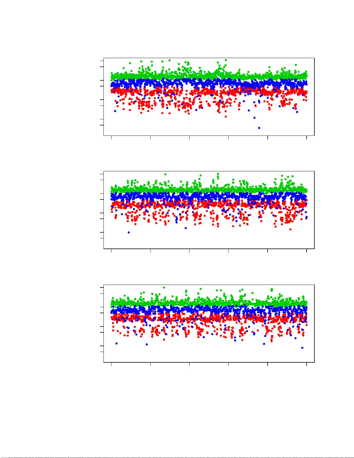
T echnical Repo rt No. 1011, D epartment of St atistics, Univ ersity of T oro n to MCMC Using Ensem bles of States f or Problems with F ast and Slo w V ariables suc h as Gaussian Pro cess Regres sion Radford M. Neal Dept. of Statistics and Dept. of Compu ter Science Univ ersit y of T oron to http://w ww.cs.uto ronto.ca/ ∼ radford/ radford@ stat.utor onto.ca 31 Decem ber 2010 Abstract. I in tro duce a Mark o v c hain Mon t e Carlo (MCMC) sc heme in which sampling from a distribution with densit y π ( x ) is done using u p dates op erating on an “ensem ble” of states. The cur ren t state x is fir st stochastic ally mapp ed to an ensemble, ( x (1) , . . . , x ( K ) ). This ensemble is then up dated using MCMC up dates that lea v e in v ariant a suitable ensemble densit y , ρ ( x (1) , . . . , x ( K ) ), defined in terms of π ( x ( i ) ) for i = 1 , . . . , K . Finally a s ingle state is sto c h astically selected f rom the ensemble after these up d ates. Suc h ensem ble MCMC up d ates can b e u seful when c haracteristics of π and the ensem b le p ermit π ( x ( i ) ) for all i ∈ { 1 , . . . , K } , to b e computed in less than K times the amount of computation time needed to compute π ( x ) for a single x . On e common situatio n of this t yp e is when c hanges to some “fast” v ariables allo w for quick re-c omputation of the d en sit y , w h ereas c hanges to other “slo w” v ariables do not. Gaussian pro cess regression mo dels are an example of this sort of p roblem, with an o v erall scaling factor for co v ariances and the n oise v ariance b eing fast v ariables. I sho w that ensem b le MCMC for Gaussian p ro cess regression m o dels can in deed sub stan tially impro v e sampling p erformance. Finally , I discuss other p ossible applications o f ensemble MCMC, a nd its relatio nship to the “ m u ltiple-try Metrop olis” method of Liu, Liang, and W ong an d the “multiset sampler” of Leman, Chen, and La vine. In tr o duction In this pap er , I in tro duce a class of Ma r k ov chain Mon te Carlo metho d s that utiliz e a state sp ace that is the K -fold Cartesian pro duct of the space of interest — ie, although our inte rest is in samp ling for x in the s p ace X , w e use MCMC up d ates that op erate on ( x (1) , . . . , x ( K ) ) in the space Y = X K . Sev eral suc h metho d s ha v e previously b een pr op osed — for example, Adaptiv e Directiv e Sampling 1 (Gilks, Rob erts, a nd George , 1994) and Paralle l T emp ering (Ge y er, 1991; Earl and Deem, 2005). Th e “ensem ble MCMC” metho d s I in tro duce here differ from these metho ds in t wo fundamen tal resp ects. First, use of the space Y = X K is temp orary — after some num b er of up dates on Y , one can switc h bac k to th e space X , p erform up d ates on that space, then switc h b ac k to Y , etc. (Of course, one migh t c h o ose to alwa ys remain in the Y space, bu t the option of switc hin g bac k and forth exists.) Secondly , th e in v ariant den sit y f or an ens emble s tate ( x (1) , . . . , x ( K ) ) in th e Y sp ace is pr op ortional to the sum of the pr ob ab ilities of the ind ividual x ( k ) (or more generally a wei gh ted sum), w hereas in the p revious metho ds mentio n ed ab ov e, th e dens it y is a pr o duct of densities f or eac h x ( k ) . As a consequence, the p r op erties of the ensemble metho ds describ ed here are quite different from those of the metho ds mentio ned ab o ve. I exp ect that use of an ensem ble MCMC method will b e adv an tageous only when, for the particular distributions b eing samp led from, and the particular ensem b les c hosen, a computational short-cut exists that allo w s computation of the densit y for all of x (1) , . . . , x ( K ) with less than K times the effort needed to compute the densit y for a single state in X . Without this computational adv an tage, it is hard to see how p erformin g up dates on X K could b e b eneficial. In th is pap er, I mostly discuss on e particular con text wher e suc h a computational sh ort-cut exists — when the distrib ution b eing sampled has the c haracteristic that after c hanges to only a sub set of “fast” v ariables it is p ossib le to re-compute the density in muc h less time than is needed when other “slo w” v ariables c hange. By using ensem b les of states in which the slo w v ariables ha v e the same v alues in all ensem ble m em b ers, th e ensem ble d ensit y can b e quic kly compu ted. In th e limit as the size of the ensemble gro w s, it is p ossible u sing su c h a metho d to ap p roac h the ideal of up dating the slo w v ariables based on their m arginal distribution, integ rating ov er the fast v ariables. I apply these fast-slo w ensem ble MCMC methods to Gaussian pro cess regression mo dels (Rasm u s sen and Williams 2006; Neal 199 9) that ha ve a co v ariance function with unkno wn parameters, whic h in a fully Ba yesia n treat men t need to b e sampled using MCMC. T he computations for such mod els require op erations on the co v ariance matrix w hose time grows in p rop ortion to n 3 , wh ere n is the num b er of observ ations. If these computations are d one using the C holesky decomp osition of the co v ariance matrix, a c hange to only the o v erall scal e of th e co v ariance function do es n ot require recomputation of the Cholesky decomp osition; hence th is s cale factor can b e a fast v ariable. If computatio ns are done b y finding the eigen ve ctors and eigen v alues of the co v ariance fu nction, b oth an o verall scale factor and the noise v ariance c an b e fast v ariables. I sho w that ensem ble MCMC with either of these app r oac hes can improv e o ver MCMC on th e original state s pace. I conclude by discussing ot her p ossible applications of ensem ble MCMC, and its relationship to the “m ultiple-try Metrop olis” metho d of Liu, Liang, and W ong (2000 ), and to the “m ultiset sampler” of Leman, Chen, and La vine (2009). MCMC with an ensem ble of states Here, I introdu ce the idea of using an ensem b le of states in general, u sing the device of sto c h astically mapping from the space of interest to another space. I also discuss sev eral wa ys of defining an ensem ble. 2 I will s u pp ose that we wish to samp le fr om a distrib ution on X with pr obabilit y d ensit y or mass function π ( x ). The MCMC a pproac h is to defin e a Mark o v c hain that has π as an in v arian t distribu tion. Pro vid ed this c hain is ergo dic, simulating the c hain from any initia l state for a suitably large num b er of trans itions will pro d uce a state whose d istribution is close to π . T o implement this strategy , we need to d efine a transition p r obabilit y , T ( x ′ | x ), for the chain to mo ve to state x ′ if it is currently in state x . Up dates made according to th is transition pr ob ab ility m ust lea v e π inv arian t: Z π ( x ) T ( x ′ | x ) dx = π ( x ′ ) (1) Sto c hastically mapping t o an ensemble and bac k. An MCMC u p date that uses an en sem ble of K states can b e view ed as pr ob ab ilistically m apping from the original space, X , to a new sp ace, Y = X K , p erforming up dates on this new space, and then mapp ing bac k to the original space. W e can formalize this “temp orary mapping” str ategy , w hic h has many other applications (Neal 2006; Neal 2010, Section 5.4), as follo ws. W e defin e a transition distribu tion, T ( x ′ | x ), on the space X as the comp osition of th ree other sto c h astic mappin gs, ˆ T , ¯ T , a nd ˇ T : x ˆ T − → y ¯ T − → y ′ ˇ T − → x ′ (2) That is, starting from t he current state, x , w e obtain a v alue in the temp orary space by sampling fr om ˆ T ( y | x ). T he target distrib ution for y ∈ Y has p r obabilit y/density function ρ ( y ). W e require that Z π ( x ) ˆ T ( y | x ) dx = ρ ( y ) (3) ¯ T ( y ′ | y ) d efines a transition on the temp orary space that lea ves ρ in v arian t: Z ρ ( y ) ¯ T ( y ′ | y ) dy = ρ ( y ′ ) (4) Finally , ˇ T gets us b ac k to the original space. It m u st satisfy Z ρ ( y ′ ) ˇ T ( x ′ | y ′ ) dy ′ = π ( x ′ ) (5) The ab o ve conditions imply that the o v erall tr an s ition, T ( x ′ | x ), will lea ve π inv ariant, and so can b e used for Marko v sampling of π . In ensemble MCMC, where Y = X K , w ith the ensemble state written as y = ( x (1) , . . . , x ( K ) ), the sto c hastic mapping ˆ T , from X to Y , is defined in terms of an ensemble b ase me asur e , a distribu tion with probability densit y or mass function ζ ( x (1) , . . . , x ( K ) ), as follo ws: ˆ T ( x (1) , . . . , x ( K ) | x ) = 1 K K X k =1 ζ − k | k ( x ( − k ) | x ) δ x ( x ( k ) ) (6) Here, δ x ( · ) is the distribution with mass concentrat ed at x . The n otation x ( − k ) refers to all comp o- nen ts of the ensem b le state other than the k ’th. The prob ab ility densit y or mass fun ction for the 3 conditional d istribution of comp onent s other than the k ’th give n a v alue for the k ’th comp onen t is ζ − k | k ( x ( − k ) | x ( k ) ) = ζ ( x (1) , . . . , x ( K ) ) / ζ k ( x ( k ) ), where ζ k is th e marginal d ensit y or mass fu n ction for the k ’th comp onent , d eriv ed fr om th e join t d istribution ζ . W e assume that ζ k ( x ) is non-zero if π ( x ) is non-zero. Algorithmically , ˆ T creates a sta te in Y by c ho osing an in d ex, k , from 1 to K , uniformly at random, setting x ( k ) to the current state, x , and fi n ally randomly generating all x ( j ) for j 6 = k fr om their conditional distrib ution under ζ giv en that x ( k ) = x . Note that ˆ T dep en d only on ζ , not on π . A simple example: As a simp le (but not useful) illustr ation, let X = [0 , 2 π ) and set K = 2. Cho ose the en s em ble b ase measur e, ζ , to b e un iform on pairs of p oints with x (2) = x (1) + ω (mo d 2 π ), for some constant ω ∈ [0 , 2 π ). (Ie, the ensemble base measure is un iform o ver pairs of p oin ts on a un it circle with the second p oin t at an angle ω coun terclockwise from the fir st.) Then ζ − 1 | 1 ( · | x (1) ) = δ x (1) + ω ( mo d 2 π ) ( · ) and ζ − 2 | 2 ( · | x (2) ) = δ x (1) − ω ( mod 2 π ) ( · ). T he algorithm for the map ˆ T is 1) pic k k uniform ly from { 1 , 2 } 2) set x ( k ) = x 3) if k = 1, set x (2) = x + ω (mo d 2 π ); if k = 2, s et x (1) = x − ω (mo d 2 π ). Ha ving defin ed ˆ T as in equation (6), the d ensit y function, ρ , for the ensemble distribution that will mak e condition (3) hold can b e deriv ed as follo ws: ρ ( x (1) , . . . , x ( K ) ) = Z π ( x ) ˆ T ( x (1) , . . . , x ( K ) | x ) dx (7) = 1 K K X k =1 ζ − k | k ( x ( − k ) | x ( k ) ) π ( x ( k ) ) (8) = 1 K K X k =1 ζ ( x (1) , . . . , x ( K ) ) ζ k ( x ( k ) ) π ( x ( k ) ) (9) = ζ ( x (1) , . . . , x ( K ) ) 1 K K X k =1 π ( x ( k ) ) ζ k ( x ( k ) ) (10) So we see that the density fun ction of ρ with resp ect to the base measure ζ is sometimes simply prop ortional to the sum of π for all the ensem b le mem b ers (wh en th e ζ k are all the same un iform distribution), and m ore generally is pr op ortional to the sum of ratios of π and ζ k . The simple example c ontinue d: ζ 1 and ζ 2 are b oth u niform o ver [0 , 2 π ). F or pairs in X 2 satisfying th e constrain t that x (2) = x (1) + ω (mo d2 π ), the ensemble densit y follo ws the prop ortionalit y: ρ ( x (1) , x (2) ) ∝ π ( x (1) ) + π ( x (2) ) (11) (The probabilit y un der ρ of a p air that violates the constrain t is of course zero.) 4 W e can let ¯ T b e any sequence of Mark o v u p dates for y = ( x (1) , . . . , x ( K ) ) that lea ve ρ inv arian t (condition (4)). W e denote the result of app lying ¯ T to y by y ′ . The simple example c ontinue d: W e might define ¯ T to b e a sequence of some pre-defined num b er of Metropolis up dates (Metrop olis, et al 1953), u sing a rand om-w alk prop osal, wh ic h from state ( x (1) , x (2) ) is ( x (1) ∗ , x (2) ∗ ) = ( x (1) + υ (mo d2 π ) , x (2) + υ (mo d2 π )), with υ b eing dra wn from a distribution symmetrical around zero, suc h as uniform on ( − π / 10 , + π / 10). Su c h a prop osal is accepted with probability min[1 , ( π ( x (1) ∗ ) + π ( x (2) ∗ )) / ( π ( x (1) ) + π ( x (2) )]. T o ret urn to a s ingle state, x ′ , from the ensem ble state y ′ = ( x (1) , . . . , x ( K ) ), w e set x ′ to one of the x ( k ) , which we select randomly with p robabilities prop ortional to π ( x ( k ) ) / ζ k ( x ( k ) ). W e can see th at this ˇ T satisfies condition (5) as follo ws: Z ρ ( y ′ ) ˇ T ( x ′ | y ′ ) dy ′ = Z " ζ ( x (1) , . . . , x ( K ) ) 1 K K X k =1 π ( x ( k ) ) ζ k ( x ( k ) ) #   K X j = 1 δ x ( j ) ( x ′ ) π ( x ( j ) ) ζ j ( x ( j ) ) . K X k =1 π ( x ( k ) ) ζ k ( x ( k ) )   dx (1) · · · dx ( K ) (12) = 1 K K X j = 1 Z δ x ( j ) ( x ′ ) π ( x ( j ) ) ζ ( x (1) , . . . , x ( K ) ) ζ j ( x ( j ) ) dx (1) · · · dx ( K ) (13) = 1 K K X j = 1 Z π ( x ′ ) ζ − j | j ( x ( − j ) | x ′ ) dx ( − j ) (14) = 1 K K X j = 1 π ( x ′ ) = π ( x ′ ) (15) The simple example c ontinue d: Since ζ 1 and ζ 2 are uniform o ver [0 , 2 π ), ˇ T simply pic ks either x (1) or x (2) with probabilities p rop ortional to π ( x (1) ) and π ( x (2) ). Some p ossible e nsembles. The ensemble b ase measure, ζ , can b e defi ned in many wa ys, some of which I will discuss h ere. Note that the usefu ln ess of these ens em bles d ep ends on whether they pro du ce an y compu tational adv an tage for th e distribution b eing sampled. This w ill b e d iscu ssed in the next sec tion for problems with fast a n d slo w v ariables, where v ariations on some of th e ensem bles discussed here w ill b e used. One p ossibility is that x (1) , . . . , x ( K ) are indep enden t and identica lly distr ib uted un der ζ , so th at ζ ( x (1) , . . . , x ( K ) ) = ζ ( x (1) ) · · · ζ ( x ( K ) ), where ζ ( x ) is the marginal distribution of all th e x ( k ) . In the conditional d istribution ζ − k | k , the comp onents other than x ( k ) will also b e indep end ent, with distribution ζ ( x ( k ) ) the same as their marginal distr ibution. Wi th this ensem b le base measure, the 5 ordering of states in the ensem ble is irrelev an t, and the mapping, ˆ T , f rom a single state to an ensemble consists of com bining the current state with K − 1 states sampled from the marginal ζ . Th e mapping, ˇ T , from the ensem ble to a single state consists of r andomly selecting a state from x (1) , . . . , x ( k ) with probabilities pr op ortional to π ( x ( k ) ) /ζ ( x ( k ) ). Rather than the x ( k ) b eing indep endent in the ens emble base mea sure, they migh t ju st b e exc h ange- able. This can b e exp ressed as the x ( i ) b eing indep enden t giv en some paramater θ , wh ic h has some “prior”, ζ ( θ ) (whic h is unrelated to th e r eal prior for a Ba y esian inference pr oblem). In other words, ζ ( x (1) , . . . , x ( K ) ) = Z ζ ( θ ) K Y k =1 ζ ( x ( k ) | θ ) dθ (16) The mapp ing ˆ T can b e implemente d b y samp lin g θ from the “p osterior” density ζ ( θ | x ( k ) = x ) ∝ ζ ( θ ) ζ ( x ( k ) = x | θ ), for k r andomly c hosen from 1 , . . . , K (though due to exc hangeabilit y , this random c hoice of k isn’t r eally necessary) and then sampling x ( j ) for j 6 = k indep endent ly f rom ζ ( x ( j ) | θ ) (whic h is the same for all j ). The marginal d istributions for the x ( k ) in the ensemble b ase measure, needed to compute ρ and to map from an ensem ble to a single state, are of course all the same when this measure is exchange able. Another possib ilit y is f or t he ensem ble base measur e on x (1) , . . . , x ( K ) to be defined b y a stationary Mark o v c hain, whic h again leads to th e x ( k ) all h a ving the same marginal distribution, ζ ( x ). F or example, if X is the reals, w e might let ζ ( x ) = N ( x ; 0 , τ 2 ), where N ( x ; µ, τ 2 ) is the normal densit y function, and ζ k +1 | k ( x ( k +1) | x ( k ) ) = N ( x ( k +1) ; x ( k ) p 1 − 1 /τ 2 , 1) for k = 1 , . . . , K − 1. Going fr om a single state to an ensemble is done b y randomly selecting a p osition, k , for the curren t state, and then sim u lating the M ark ov c hain forward fr om x ( k ) to x ( K ) and bac kw ard from x ( k ) to x (1) (whic h will b e the same as forwa r d sim ulation when the chain is r ev ersible, as in the example here). The ensem ble densit y is giv en by equation (10), with all th e m arginal d ensities ζ k ( x ) equal to ζ ( x ). W e return from an ensemble to a sin gle state by selecting f r om x (1) , . . . , x ( k ) with probabilities prop ortional to π ( x ( k ) ) /ζ ( x ( k ) ). Ensem ble b ase measures can also b e defin ed usin g c onstel lations of p oints. Let x (1) ∗ , . . . , x ( K ) ∗ b e some set of K p oints in X . W e let ζ b e the distribu tion obtained by shifting all these p oints b y an amoun t, θ , c hosen from some distribu tion on X , with densit y ζ ( θ ) that is no wh er e zero, so that ζ ( x (1) , . . . , x ( K ) ) = Z ζ ( θ ) K Y k =1 δ x ( k ) ∗ + θ ( x ( k ) ) dθ (17) The conditional distributions ζ − k | k do n ot d ep end on ζ ( θ ) — they are degenerate distrib utions in whic h the other constellati on points are determined by x ( k ) . W e therefore mo ve from a single p oin t, x , to a constella tion of points b y selecting k at random from 1 , . . . , K , setting x ( k ) to x , and setting x ( j ) for j 6 = k to x ( j ) ∗ + x − x ( k ) ∗ . The ensemble density , ρ ( x (1) , . . . , x ( K ) ), will also not dep end on ζ ( θ ), as can b e s een from equatio n (8)) — it will b e prop ortional to th e sum of π ( x ( k ) ) for ensembles that hav e the shap e of the constellation, and b e zero for those that d o not. The marginal d en sities, ζ k ( x ( k ) ), w ill b e the sa me for all constellatio n p oints, since θ = x ( k ) − x ( k ) ∗ will b e the same for all k . (Note th at this is not the same as the marginal densit y fun ctions b eing the same for all k .) Hence mo ving to a single 6 p oint from a constella tion is d one by c ho osing a p oin t, x ( k ) , from the constellation with pr obabilities prop ortional to π ( x ( k ) ). The simp le example used in the p revious section can b e s een as a constellatio n of t wo p oin ts with x (1) ∗ = 0, x (2) ∗ = ω , ζ ( θ ) uniform o ver [0 , 2 π ), and addition don e m o dulo 2 π . In the p resen tation abov e, the ensem ble base m easure ζ is assumed to b e a p rop er pr obabilit y distribution, but ζ can instead b e an i mprop er limit of pr op er distribu tions, as long as the co nditional distributions and ratios of marginal distributions that are n eeded ha v e su itable limits. In particular, the conditional distributions ζ − k | k used to define ˆ T in equation (6) must reac h limits th at are pr op er distributions; this will also en sure that ρ is w ell defined (see equatio n (8)). The ratios ζ j ( x ( j ) ) / ζ k ( x ( k ) ) m u st also reac h limits, so that ˇ T will b e well defined. W e can obviously let ζ ( θ ) b ecome improp er w hen d efining a constellatio n ensemble, sin ce we ha v e seen that the c h oice of this density h as no effect. F or exc hangeable ensem bles, w e can let ζ ( θ ) b e improp er as long as the “p osterior”, ζ ( θ | x ( k ) = x ), is prop er. W e can also let τ go to infin - it y in the Mark o v ens emble base m easur e defined ab o ve. W e w ill th en ha ve ζ k +1 | k ( x ( k +1) | x ( k ) ) = N ( x ( k +1) ; x ( k ) , 1), s o the conditional d istributions ζ − k | k are simple r andom walks in b oth directions from x ( k ) . Since the m arginal distributions for the x ( k ) are all norm al with mean zero and v ariance τ 2 , for an y x ( j ) and x ( k ) , th e ratio ζ ( x ( j ) ) / ζ ( x ( k ) ) approac h es one as τ goes to in finit y . (Note also that since the limit of ζ − k | k is prop er, the r elev an t v alues of x ( k ) will not div erge, so uniform con vergence of these ratios is not necessary .) Ensem ble MCMC for problems with “fast” and “slow” v ariables Supp ose that w e wish to s ample from a distrib ution on a space that can b e written as a C artesian pro du ct, X = X 1 × X 2 , with element s written as x = ( x 1 , x 2 ). S upp ose also that the p robabilit y densit y or mass fun ction, π ( x 1 , x 2 ), is suc h that re-computing the d ensit y afte r a c h ange to x 2 is muc h faster th an rec omputing the density after a change to x 1 . That is, if w e ha ve computed π ( x 1 , x 2 ), and sa ved suitable in termediate results from this computation, we can quic kly compute π ( x 1 , x ′ 2 ) for an y x ′ 2 , b ut there is no short-cut for compu tin g π ( x ′ 1 , x ′ 2 ) for x ′ 1 6 = x 1 . In general, x 1 and x 2 migh t b oth b e multidimensional. I refer to x 1 as the “slo w” v ariables, and x 2 as the “fast” v ariables. I first encount ered this class of prob lems in conn ection with mo dels for the C osmic Micro wa ve Bac kground (CMB) radiation (Lewis and Bridle, 200 2). This is an example of data mo delled using a complex sim ulation, in this case, of the early u niv ers e. In su c h p roblems, the slo w v ariables, x 1 , are the un kno wn p arameters of the simulat ion, w hic h are b eing fit to observ ed data. Wh en new v alues for these parameters a re considered, as for a M etrop olis p rop osal, computing π with these new v alues will require re-runnin g the sim ulation, wh ich w e assume tak es a large amoun t of computation time. Some fairly simple mo del r elates the output of the sim u lation to the observ ed data, with parameters x 2 (for example, the noise lev el of the observ ations). When a new v alue for x 2 is considered in conju nction with a v alue for x 1 that was previously considered, the sim u lation d o es not need to b e re-run , assum ing the output from the p revious run w as sa ved. In stead, computing π with th is new x 2 and the old x 1 requires only some muc h faster calculat ion in volving the observ ation m o del. 7 F ast and slo w v ariables arise in many other cont exts as w ell. F or example, in man y Bay esian m o dels, the p osterior dens ity for a set of lo w-lev el parameters inv olv es a large num b er of data items, wh ic h cannot b e summarized in a few sufficient statistics, while a small num b er of hyperp arameters hav e densities that dep end (directly) only on the lo w-lev el parameters. The lo w -lev el parameters in s u c h a situation will b e “slo w”, sin ce when they are c hanged, all the data items m ust b e look ed at again, but the hyperp arameters may b e “fast”, since when they change, but the lo w-lev el parameters sta y the same, ther e is no need to lo ok at the data. Later in th is pap er, I w ill consider app lying metho ds for fast and slo w v ariables to the more sp e- cialize d p roblem of sampling fr om the p osterior distribution of the parameters of a Gaussian pro cess regression m o del, in w hic h an o verall scale factor for the co v ariance fu nction and the n oise v ariance can b e regarded as fast v ariables. Previous met ho ds for problems with fast and slo w v ariables. A simp le w ay of exploiting fast v ariables, used by Lewis and Bridle (2002), is to p erform extra Metrop olis up dates that c hange only the fast u p dates, along with less frequent up d ates that c hange b oth f ast and slo w v ariables. Lewis and Bridle foun d that this is an impro v ement o v er alw a ys p erforming up d ates for all v ariables. Similarly , w hen using a Metrop olis metho d that up dates only one v ariable at a time, one could p erform more up dates for the fast v ariables than for the slow v ariables. I w ill refer to these as “extra up date Metrop olis” metho d s . Another simple fast-slo w method I devised (that has b een found useful for the CMB mo deling problem) is to rand omly choose a d isplacemen t in th e slo w sp ace, δ 1 ∈ X 1 , and then p erform s ome pre-determined n umb er of Metrop olis up d ates in whic h the prop osal from state ( x 1 , x 2 ) is ( x 1 ± δ 1 , x ′ 2 ), where the sign b efore δ 1 is c hosen randomly , and x ′ 2 is c hosen from some suitable prop osal distrib ution, p erhaps d ep ending on x 1 , x 2 , and the chosen sign for δ 1 . During suc h a sequence of “random grid Metrop olis” up dates, all prop osed and accepted states will ha ve slow v ariables of th e form x 1 + iδ 1 , where x 1 is the in itial v alue, and i is an integ er. If inte rmediate results of compu tations with all these v alues for the slo w v ariables are sa ved, th e num b er of slo w computations ma y be m uc h less than the num b er of Metrop olis p rop osals, since the same slow v ariables ma y b e prop osed many times in conjunction with different v alues for the fast v ariables. If recomputation after a change to the fast v ariables is v ery muc h faster than after a c h an ge to the slo w v ariables, w e migh t hop e to fin d an MCMC metho d that samples n early as efficien tly as w ould b e p ossible if we could efficien tly compute the margi nal distribution for just the slo w v ariables, π ( x 1 ) = R π ( x 1 , x 2 ) dx 2 , since we could appr o ximate this in tegral usin g man y v alues of x 2 . I ha ve devised a “dragging Metrop olis” metho d (Neal, 2004) that can b e seen as attempting to ac hieve this. The ensemble MCMC metho ds I describ e next can also b e view ed in this wa y . Applying ensem ble MCMC to problems wit h fa st and slow v ariables. En sem ble MCMC can b e applied to this problem using ensem bles in w h ic h all state s ha ve the same v alue for the slow v ariables, x 1 . Comp utation of the ensem ble probability densit y (equation (10)) can then tak e a d v an tage of quick computation for multiple v alues of the f ast v ariables. Man y sampling sc hemes of this sort are possib le, 8 distinguished b y the ensemble base measure used, and by the up dates that are p erformed on the ensem b le (ie, by the transition ¯ T ) . F or all the schemes I ha v e lo ok ed at, the fast and slo w v ariables are indep endent in th e base ensem b le measure used, and the slo w v ariables hav e the same v alue in all mem b ers of the ensemble. The ensemble base measure therefore has the follo wing form: ζ ( x (1) , . . . , x ( K ) ) = h ω ( x (1) 1 ) K Y k =2 δ x (1) 1 ( x ( k ) 1 ) i ξ ( x (1) 2 , . . . , x ( K ) 2 ) (18) Here, ω ( x 1 ) is some densit y for the slo w v ariables — the c h oice of ω will tur n out not to matter, as long as it is no where zero. Th at the slo w v ariables h a ve th e same v alues in all ensem b le mem b ers is expressed by the factors of δ x (1) 1 ( x ( k ) 1 ). The joint distribution of the fast v ariables in the K mem b ers of the ensemble is giv en b y the densit y function ξ . If we let ξ k b e the marginal distribution for the k ’th mem b er of the ens em ble under ξ , we can write the ensem ble d ensit y f r om equation (10) as follo ws: ρ ( x (1) , . . . , x ( K ) ) = ζ ( x (1) , . . . , x ( K ) ) 1 K K X k =1 π ( x ( k ) ) ζ k ( x ( k ) ) (19) = h K Y k =2 δ x (1) 1 ( x ( k ) 1 ) i ξ ( x (1) 2 , . . . , x ( K ) 2 ) 1 K K X k =1 π ( x ( k ) ) ξ k ( x ( k ) 2 ) (20) P ossible c hoices for ξ include th ose analogous to some of the general c hoices for ζ discussed in the previous section, in particular the follo win g: indep enden t Let x (1) 2 , . . . , x ( K ) 2 b e indep end ent under ξ , with all ha ving the same marginal d istribution. F or example, if th e f ast v ariables are parameters in a Ba ye sian m o del, w e migh t use their pr ior distribution. exc hangeable Let x (1) 2 , . . . , x ( K ) 2 b e exc h an geable u nder ξ . If x 2 is s calar, we migh t let x ( k ) 2 | θ ∼ N ( θ , τ 2 ) and θ ∼ N (0 , ψ 2 ). W e could then let ψ go to infinit y , so that ξ is im p rop er, and all ξ k are the same. grid p oin ts Let x ( k ) 2 = x ( k ) ∗ + θ for k = 1 , . . . , K . Here, if x 2 has dimension D , θ is a D -dimensional offset that is ap p lied to the s et of p oin ts x ( k ) ∗ . This is an examp le of a constellation, as discussed in the previous section. One p ossibility is a r ectangular grid, with K = m D for some intege r m , and with grid p oin ts spaced a distance d j in d im en sion j , so that the e xten t of the grid in d imension j is ( m − 1) d j . The ensemble up date, ¯ T , could b e done in man y w a ys , as long as the up date lea v es ρ inv arian t. A simple and general option is to p erform some num b er of Metrop olis-Hastings u p dates (Metrop olis, et al 9 1953; Hastings 19 70), in which we prop ose to c h ange the curren t ensemble s tate, y = ( x (1) , . . . , x ( K ) ), to a prop osed s tate, y ∗ , drawn according to some prop osal densit y g ( y ∗ | y ). W e acc ept the pr op osed y ∗ as the n ew state with p r obabilit y min[ 1 , ρ ( y ∗ ) g ( y | y ∗ ) / ρ ( y ) g ( y ∗ | y ) ], where ρ is defined by equation (2 0). A tec hnical issue arises wh en X is contin uous — since x ( k ) 1 m u st b e the same for all memb ers of the ensem b le, the probabilit y densities will b e infi nite (eg , due to the delta functions in equation (20)). W e can a vo id this by lo oking a t densities for only x (1) 1 and x (1) 2 , . . . , x ( K ) 2 , since x (2) 1 , . . . , x ( K ) 1 are just equal to x (1) 1 . (This assumes that w e nev er prop ose states violating this constraint .) A similar iss ue arises when using an ensemble of grid p oints, as d efined ab o ve, in which the x ( k ) 2 are constrained to a grid — here also, we can simply lea ve out the infinite factors in the dens it y that enforce the deterministic constrain ts, assuming that our pr op osals nev er violate them. I will consider tw o classes of Metrop olis up dates for the ensemble state, in whic h symmetry of the prop osal mak es g ( y | y ∗ ) /g ( y ∗ | y ) equal to on e, so the acceptance p robabilit y is min[ 1 , ρ ( y ∗ ) /ρ ( y ) ]: fast v ariables fixed Prop ose a new v alue for x 1 in all ensemble members , by adding a rand om offset dra w n fr om some symmetrical distribution to the current v alue of x 1 . Keep the v alues of x (1) 2 , . . . , x ( K ) 2 unc hanged in the p rop osed state. fast v ariables shifted Prop ose a new v alue for x 1 in all ensemble memb ers as ab o ve , together with new v alues for x (1) 2 , . . . , x ( K ) 2 found by adding an offset to all of x (1) 2 , . . . , x ( K ) 2 that is randomly dr a wn from some symmetrical distr ibution. These tw o s chemes are i llustrated in Figure 1. E ith er sc heme could b e com bined with an y of the three Figure 1: Illustration of ensem ble u p dates with w ith one slow v ariable (horizont al) and one fast v ariable (v ertical). The distribution is u niform ov er the outlined region. A grid ensem ble with K = 10 is used. On the le ft, a mo v e is prop osed by c hanging only the slo w v ariable; it w ill be accepted with probabilit y 1 / 4, since four members of the cur ren t ensem ble hav e non-zero probability , compared with only one in the prop osed ens emble. On the r igh t, a mo ve is prop osed by c hanging the slo w v ariable and also shifting the grid ensem ble; it will b e accepte d with probabilit y 2 / 4. (Of course, a less fa v our able shift in the grid ensem ble m igh t ha v e led to zero p robabilit y of acce ptance.) 10 t yp es of ensembles ab o ve, bu t shifting the fast v ariables when th ey are sampled indep enden tly f r om some distr ib ution s eems unlike ly to w ork we ll, since after sh ifting, the v alues for the fast v ariables w ould not b e typica l of th e distribution. One could p erform just one Metrop olis up date on th e ensem ble s tate b efore return in g to a single p oint in X , or man y such up d ates could b e p erform ed . Mo ving bac k to a sin gle p oin t an d then regenerating an ensemble b efore p erforming the next en sem ble up date will requires some compu tation time, but ma y impro v e sampling. Up dates migh t a lso b e p erf ormed on X (p erh aps c han ging only fast v ariables) b efore mo ving bac k to an ensem ble. F ast and slo w v ariables in Gaussian pro cess regression mo dels Gaussian process regression (Neal 1999; Rasmussen and Williams, 2006) is one cont ext where ensem ble MCMC can b e applied to facilitate samp ling when there are “fast” and “slo w” v ariables. A brief in tro duction to Gaussian pro cess regression. Supp ose that w e observ e pairs ( z ( i ) , y ( i ) ) for i = 1 , . . . , n , w here z ( i ) is a v ector of p co v ariates, whose distrib u tion is not mo deled, and y ( i ) the corresp onding real-v alued resp onse, whic h w e mo del as y ( i ) = f ( z ( i ) ) + e ( i ) , w here f is an un k n o wn function, and e ( i ) is indep endent Gauss ian noise with mean zero and v ariance σ 2 . W e can give f a Gaussian pro cess prior, w ith mean zero and some cov ariance fun ction C ( z , z ′ ) = E [ f ( z ) f ( z ′ )]. W e then base pred iction f or a future observ ed resp onse, y ∗ , asso ciated with co v ariate v ector z ∗ , on the conditional distribution of y ∗ giv en y = ( y (1) , . . . , y ( n ) ). This cond itional distribution is Gaussian, with mean and v ariance th at can b e computed as follo ws: E ( y ∗ | y ) = k T Σ − 1 y , V ar ( y ∗ | y ) = v − k T Σ − 1 k (21) Here, Σ = K + σ 2 I is the co v ariance matrix of y , with K ij = C ( z ( i ) , z ( j ) ). Co v ariances b etw een y ∗ and y are giv en by the v ector k , with k i = C ( z ∗ , z ( i ) ). The marginal v ariance of y ∗ is v = C ( z ∗ , z ∗ ) + σ 2 . If the co v ariance function C and the noise v ariance σ 2 are known, th e matrix op erations ab ov e are all that are needed f or inference and pr ediction. Ho wev er, in practice, th e n oise v ariance is not known, and the co v ariance f unction w ill also hav e un k n o wn p arameters. F or example, one commonly-used co v ariance function has the form C ( z , z ′ ) = η 2  a 2 + exp  − p X h =1  ν h ( z h − z ′ h )  2  (22) Here, the a 2 term allo ws for th e o ve rall lev el of the fu n ction to b e shifted up w ard s or do wnw ards from zero; it migh t b e fixed a priori . Ho we v er, we t ypically do not kno w wh at are suitable v alues f or the parameter η , wh ic h expresses the magnitude of v ariation in the fun ction, or f or the parameters ν 1 , . . . , ν p , which express ho w relev ant eac h co v ariate is to predicting th e resp on s e (with ν h = 0 indicating that z h has no effect on p redictions for y ). In a fully Ba yesian treatme n t of this mo del, η , ν , and σ are giv en prior distributions. Indep en d en t Gaussian prior distributions for the log of eac h p arameter ma y b e suitable, with means and v ariances 11 that are fixed a priori . In the mo dels I fit b elo w , the logs of the comp onents of ν are correlated, whic h is appropr iate when learning that one co v ariate is highly relev an t to pr ed icting y increases our b elief that other co v ariates migh t also b e relev ant. After sampling th e p osterior d istribution of the parameters with some MCMC metho d, predictions for future observ ations can b e made b y a verag in g the Gaussian distr ib utions giv en b y (21) o ver v alues of the parameters tak en from the MCMC r un. Sampling from the p osterior distrib ution requires the like liho o d for the parameters giv en the data, whic h is simply the Gaussian probabilit y densit y for y with these parameters. The log lik eliho o d, omitting constant terms, can therefore b e written as log L ( η, ν , σ ) = − (1 / 2 ) log det Σ( η , ν , σ ) − (1 / 2 ) y T Σ( η , ν, σ ) − 1 y (23) This log likeli ho o d is u sually computed by findin g the Ch olesky decomp osition of Σ, which is the lo we r-triangular matrix L f or which LL T = Σ. F rom L , b oth terms ab ov e are easily calculated. In the first term, the determinant of Σ can b e found as (d et L ) 2 , with det L b eing ju st the pro du ct of the diagonal en tries of L . In the second term, y T Σ − 1 y = y T ( LL T ) − 1 y = u T u , w here u = L − 1 y can b e found by forw ard sub stitution. Computing the Cholesky decomp osition of Σ requires time p rop ortional to n 3 , with a rather small constan t of pr op ortionalit y . Compu tation of Σ requires time prop ortional to n 2 p , w ith a somewhat larger constan t of p rop ortionalit y (which ma y b e larger still when co v ariance fu nctions more co mplex than equation (22) are used). I f p is fi xed, the time for the Cholesky deco m p osition will dominate for large n , b ut for mo derate n (eg, n = 10 0, p = 10), the time to compute Σ ma y b e great er. Expressing computations in a form with fast v a ria bles. I will sho w here how th e lik eliho o d for a Gaussian pr o cess regression mo del can b e rewr itten so that some of the unkn o wn parameters are “fast”. Sp ecifically , if computations are done u sing the Cholesky d ecomp osition, η can b e a fast parameter, and if compu tations are instead done b y fin d ing the eigenv ectors and eigen v alues of the co v ariance matrix, b oth η and σ can b e fast parameters. Note that the MC MC metho ds u sed w ork b etter wh en applied to the logs of the p arameters, s o the actual f ast parameters will b e log( η ) and log( σ ), though I sometimes omit the logs when referr ing to them here. The form of co v ariance f unction sho w n in equation (22) has already b een d esigned so that η can b e a fast parameter. Previously , I (and others) h av e used cov ariance functions in which the constant term a is not m ultiplied b y the scale factor η 2 , bu t writing it as in equation (22) will b e essen tial for η to b e a fast parameter. As an expr ession of prior b eliefs, it mak es little difference whether or n ot a 2 is m ultiplied by η 2 , since a is t y p ically c hosen to b e large enough th at an y reasonable shift of th e function is p ossible, ev en if a is m ultiplied b y a v alue of η at the lo w end of its prior range. Indeed, one could let a go to infin it y — analogous to letting the prior for the int ercept term in an ord inary linear regression model b e improp er — without causing any significant s tatistica l problem, although in practice, to a voi d numerical problems from near-singularit y of Σ, excessiv ely large v alues of a should b e a vo id ed. A large v alue for a will b e usually b e unnecessary if the resp onses, y , are cen tr ed to ha ve sample mean zero. T o mak e η a f ast v ariable wh en usin g Cholesky compu tations, we also need to rewrite the cont ri- 12 bution of the noise v ariance to Σ as η 2 times σ 2 /η 2 = ψ 2 . W e w ill then d o MCMC with log( η ) as a fast v ariable and log ( ψ ) and log ( ν h ) f or h = 1 , . . . , p as slo w v ariables. (Note that the Jacobian for the transformation from (log( η ) , log ( σ )) to (log( η ) , log ( ψ )) has determinan t one, so no adjustmen t of p osterior densities is required with this transf ormation.) F ast r ecompu tation of the lik eliho o d after η c h anges can b e done if we write Σ = η 2 (Υ + ψ 2 I ), where Υ ij = a 2 + exp  − p X h =1  ν h ( z ( i ) h − z ( j ) h )  2  (24) Υ + ψ 2 I is not a fun ction of log( η ), but only of log( ψ ) and the log ( ν h ). Giv en v alues for these slo w v ariables, we can compute the Cholesky d ecomp osition of Υ + ψ 2 I , and from that det(Υ + ψ 2 I ) and y T (Υ + ψ 2 I ) y , as describ ed earlier. If these results are sav ed, for any v alue of the fast v ariable, lo g ( η ), w e can quic kly compu te det Σ = η 2 n det(Υ + ψ 2 ) and y T Σ − 1 y = y T (Υ + ψ 2 I ) − 1 y / η 2 , whic h suffi ce for computing th e likeli ho o d. Rather than use the Cholesky decomp osition, we could instead compute the like liho o d for a Gaus- sian pro cess mo del by fi n ding the eigen vecto rs and eigen v alues of Σ. Let E b e the matrix w ith th e eigen v ectors (of u nit length) as columns, and let λ 1 , . . . , λ n b e the corresp onding eigen v alues. The pro jections of the data on the eigen v ectors are gi v en by u = E T y . Th e log likeli ho o d of (23) can then b e computed as follo ws: log L = − 1 2 n X i =1 log λ i − 1 2 n X i =1 u 2 i λ i (25) Both finding the Cholesky deco mp osition of an n × n matrix and finding its eige n vecto r s and e igen v alues tak e time prop ortional to n 3 , but the constant factor f or finding the C h olesky decomposition is smaller than for find in g the eigen ve ctors (b y ab out a factor of fifteen), h ence the usual p reference for u sing the Cholesky d ecomp osition. Ho we v er, if computations are done using eigen v ectors an d eigen v alues, b oth η and σ can b e m ad e fast v ariables. T o d o this, we write Σ = η 2 Υ + σ 2 I . Giv en v alues for the slo w v ariables, log ( ν h ) for h = 1 , . . . , p , we can compute Υ, and then find its eigen v alues, λ 1 , . . . , λ n , and the pro j ections of y on eac h of its eigen v ectors, wh ic h will b e denoted u i for i = 1 , . . . , n . If w e sa v e these λ i and u i , we can quic kly compute L f or an y v alues of η and σ . The eigenv ectors of Σ are the same as th ose of Υ, and the eigen v alues of Σ are η 2 λ i + σ 2 for i = 1 , . . . , n . Th e log lik eliho o d for the log ( ν h ) v alues used to compute Υ along w ith v alues for the fast v ariables log ( η ) and log( σ ) can therefore b e f ou n d as log L = − 1 2 n X i =1 log ( η 2 λ i + σ 2 ) − 1 2 n X i =1 u 2 i η 2 λ i + σ 2 (26) This pro cedure m ust b e mo difi ed to a v oid numerical difficulties when Υ is nearly singular, as can easily happ en in practice. The fix is to add a small amoun t to the diagonal of Υ, giving Υ ′ = Υ + r 2 I , where r 2 is a sm all amount of “jitter”, and then usin g Υ ′ in the computations describ ed ab o ve . T he statistica l effect of this is that the n oise v ariance is changed to η 2 r 2 + σ 2 . By fixing r to a su itably small v alue, the difference of this from σ 2 can b e made negligible. F or consistency , I also use Υ ′ for 13 the C holesky metho d (so the Cholesky decomp osition is of Υ ′ + ψ 2 I ), ev en though adding jitter is necessary in that con text only when ψ 2 migh t b e v ery small. T o summ arize, if w e u se the Cholesky decomp osition, we can compute the lik eliho o d for all mem b ers of an ensem ble differing only in η u sing only sligh tly more time than is n eeded to compute the like li- ho o d for one p oin t in the u s ual wa y . Only a small a moun t of additional time, indep end en t of n a nd p , is needed for eac h mem b er of the ensem ble. Computation of eigen v ectors is ab out fifteen time s slo w er than the Cholesky decomp osition, and compu ting the lik eliho o d for eac h ensem b le mem b er using these eigen v ectors is also slo wer, taking time p rop ortional to n . Ho wev er, when u sing eigen vect or compu- tations, b oth η and σ can b e fast v ariables. Wh ich method will b e b etter in practice is unclear, and lik ely dep ends on the v alues of n and p — for mod er ate n and large p , time to compute the co v ariance matrix, w hic h is th e same for b oth metho d s, will dominate, fa vo u ring eigen v ector computations that let σ b e a fast v ariable, wh ereas for large n and small p , th e smaller time to compu te the Cholesky decomp osition may b e the dominant consideration. If w e wish to use a small ensem ble o ver b oth η and σ , it ma y sometimes b e desir ab le to do the computations u sing the Cholesky decomp osition, recomputing it for ev ery v alue of the fast v ariables. This w ould make sense only if the time to compute the co v ariances (apart from a final scaling by η 2 and addition of σ 2 I ) dominates the time for these multiple Cholesky computations (otherwise usin g the e nsem b le will not b e b eneficial), and the ensem ble has less than about fifteen mem b ers (o therwise a single eige n vecto r computation would b e faster). Ho wev er, I do not consid er this p ossibilit y in the demonstraton b elo w, where larger ensem bles are used. A demonstration Here, I demonstrate and compare standard Metrop olis and ensem b le MCMC on the problem of sam- pling from the posterior distribution for a Gaussian p ro cess regression mo del, using the fast-slo w metho ds describ ed ab o ve . The mo d el and syn th etic test data that I u se w ere c h osen to pro d uce an inte resting p osterior distribu tion, ha v in g seve ral mo des that corresp ond to differen t d egress of predictabilit y of the resp onse (and hence different v alues for σ ). The MCMC p rograms w ere written in R, and run on t w o mac hines, with tw o versions of R — v ersion 2.8.1 on a Solaris/SP AR C mac hine, and v er s ion 2.12.0 on a L in u x /Intel mac hine. Th e programs used are a v ailable at m y w eb site. 1 The syn thet ic data. In the generated d ata, the tru e relationship of the resp onse, y , to the vect or of co v ariates, z , w as y = f ( z ) + e , with e b eing indep endent Gaussian noise with standard deviatio n 0 . 4, and the r egression function b eing f ( z ) = 0 . 7 z 2 1 + 0 . 8 s in (0 . 3 + (4 . 5 + 0 . 5 z 1 ) z 2 ) + 0 . 85 cos (0 . 1 + 5 z 3 + 0 . 1 z 2 2 ) (27) The n u mb er of co v ariates wa s p = 12, though as seen ab o ve, f ( z ) dep ends only on z 1 , z 2 , and z 3 . The co v ariate v alues w ere r andomly dra wn from a m ultiv ariate Gaussian distribu tion in wh ic h all the 1 http://www .cs.utoro nto.ca/ ∼ radf ord/ 14 z h had m ean zero and v ariance one. There were wea k correlati ons among z 1 , z 2 , an d z 3 . There we re strong (0 .99) correlations b et ween z 1 and z 4 , z 2 and z 5 , an d z 3 and z 6 , an d mo derate (0.9) correlato ns b et ween z 1 and z 7 , z 2 and z 8 , and z 3 and z 9 . Co v ariates z 10 , z 11 , and z 12 w ere ind ep endent of eac h other and the other co v ariates. 2 I generated n = 100 indep endent pairs of cov ariate v ectors and resp onse v alues in this wa y . The Gaussian pro cess mo del. Th is synthetic data wa s fit with a Gaussian pro cess r egression mo del of the sort describ ed in the previous section, in wh ic h the pr ior co v ariance b et we en resp onses y ( i ) and y ( j ) w as Co v( y ( i ) , y ( j ) ) = η 2  a 2 + exp  − p X h =1  ν h ( z ( i ) h − z ( j ) h )  2  + r 2 δ ij  + σ 2 δ ij (28) where δ ij is zero if i 6 = j and one if i = j . I fixed a = 1 and r = 0 . 01. The p riors for η , σ , and ν w er e indep end en t. The prior for log( σ ) w as Gaussian with mean log(0 . 5) and standard deviation 1.5; that for log( η ) was Gaussian with mean o f log (1) and standard deviation 1.5. Th e prior f or ν wa s multiv ariate Gaussian with eac h log( ν h ) h a ving mean log (0 . 5) and standard deviation 1 .8, and with the correlat ion of ν h and ν h ′ for h 6 = h ′ b eing 0 . 6 9. Ha vin g a non-zero prior correlation b etw een the ν h is equiv alent to usin g a pr ior expressed in terms of a h igher-lev el h y p erparameter, ν 0 , conditional on whic h th e ν h are indep end en t with m ean ν 0 . P erformance of standard Metrop olis s ampling. I tried sampling from the p osterior distribu tion for this m o del and d ata using standard r an d om-w alk Metrop olis metho d s, with th e state v ariables b eing the logs of the parameters of the co v ariance function (the tw elv e ν h parameters, η , and σ ). I fir st tried using a multiv ariate Gaussian Metrop olis prop osal distrib ution, centred at the curren t state, with ind ep endent c h anges for eac h v ariable, with th e same standard deviation — ie, the prop osal distribution was N ( x, s 2 I ), where x is the cu r ren t state, and s is the prop osal standard deviation. Figure 2 shows results with s = 0 . 25 (top) and s = 0 . 35 (bottom). Th e plots sho w three quan tities, on a logarithmic scale, f or every 300th iteration from a total of 300,000 Metrop olis u p dates (so that 1000 p oint s are p lotted). The quan tity sho w n in red is the a verage of th e ν h parameters (giving relev ances of the co v ariates), that shown in green is th e η parameter (the o ve r all scale), and that sho w n in blue is the σ parameter (noise standard d eviation). When s = 0 . 2 5, the rejection rate is 87%. F rom the top plot, it app ears that the chai n has con v erged, and is sampling from t wo mo des, c haracterized by v alues of σ around 0.5, or muc h smaller v alues. Mo v emen t b et ween these mo d es o ccurs fairly infr equen tly , b ut an adequate samp le app ears to ha ve b een obtained in 300,000 iterations. 2 In detail, the co v ariates w ere generated by letting w h for h = 1 , . . . , 12 b e indep endent standard normals, and then letting z 1 = w 1 , z 2 = 0 . 25 z 1 + w 2 √ 1 − 0 . 25 2 , z 3 = 0 . 25 z 2 + w 3 √ 1 − 0 . 25 2 , z 4 = 0 . 99 z 1 + w 4 √ 1 − 0 . 99 2 , z 5 = 0 . 99 z 2 + w 5 √ 1 − 0 . 99 2 , z 6 = 0 . 99 z 3 + w 6 √ 1 − 0 . 99 2 , z 7 = 0 . 9 z 1 + w 7 √ 1 − 0 . 9 2 , z 8 = 0 . 9 z 2 + w 8 √ 1 − 0 . 9 2 , z 9 = 0 . 9 z 3 + w 9 √ 1 − 0 . 9 2 , z 10 = w 10 , z 11 = w 11 , and z 12 = w 12 . 15 s = 0 . 25 : 0 50000 100000 150000 200000 250000 300000 5e−03 1e−01 5e+00 average nu / eta / sigma average nu eta sigma s = 0 . 35 : 0 50000 100000 150000 200000 250000 300000 5e−03 1e−01 5e+00 average nu / eta / sigma average nu eta sigma Figure 2: Runs u sing Metropolis up dates of all parameters at once, with t w o v alues for the p rop osal standard deviation, s . Ho we v er, the b ottom p lot sho w s that this is n ot the case. T h e rejection rate here, with s = 0 . 3 5, is high, at 94%, but this c hain explores additional mod es that w ere m issed in the run with s = 0 . 25. The sample from 300,0 00 it erations is nev erth eless far f rom adequate. Some mod es w ere m o ve d to and from only once in the run, so an acc urate estimate of the probalit y of ea c h mo de cannot b e obtained. Metrop olis up dates that c hange only one parameter at a time, systematicall y up d ating all pa- rameters once p er MCMC iteration, p erform b etter. (This is presum ably b ecause in the p osterior distribution there is fairly lo w dep endence of some parameters on others, so that fairly large c hanges can sometimes be made to a single parameter.) Up d ating a ν h parameter is slo w, requiring ab out the same computation time as an up date c hanging all parameters. Ho w ever, u p dates that c hange only η , or (if computations are done using eigen v ectors) only σ , will b e f ast. T o allo w a fair comparison, the n u m b er of iterations done was set so that the num b er of slo w ev aluations w as 300,000 , the same as for the ru ns with Metrop olis up dates of all v ariables at once. T o make the comparison as f a v ourable 16 0 5000 10000 15000 20000 25000 5e−03 1e−01 5e+00 average nu / eta / sigma average nu eta sigma Extra: 0 5000 10000 15000 20000 25000 5e−03 1e−01 5e+00 average nu / eta / sigma average nu eta sigma Figure 3: Runs using Metrop olis up d ates of one parameter at a time, with extra up d ates of fast parameters for the low er plot. as p ossible for this metho d, I assumed that computations are d one using eigen v ectors, so that b oth η and σ are fast v ariables. The top plot in Figure 3 shows results u sing suc h single-v ariable Metrop olis up dates (selected as among the b est of runs with v arious settings that w ere tried). Here, the prop osal standard deviation w as 2 for the ν h parameters, and 0.6 for the η and σ parameters. (Recall that all p arameters are represent ed by their logs.) The rejection rates for the u p dates of the v ariables ranged from 53% to 77%. O ne can see that sampling is significan tly impro ve d, but that some modes are still visited o nly a few times durin g the run . On e wa y to try to imp r o ve sampling further is to p erform additional up dates of the fast v ariables. The b ottom plot in Figure 3 sh o ws the results when 49 add itional Metrop olis up d ates of the fast v ariables ( η and σ ) are done eac h iteration. This seems to p ro duce little or no impro v ement on this problem. (Ho wev er, on some other problems I ha ve tried, extra up dates of fast v ariables do impro ve sampling.) 17 The time requir ed for a slo w ev aluation usin g computations based on the Cholesky decomp osition w as 0.0081 seconds on the Intel machine, and 0.0661 seconds on the SP AR C mac hine. When u sing computations based on eigen v ectors, a slow ev aluation to ok 0.0128 seconds on the Int el mac hine, and 0.0886 seconds on the S P ARC m ac hine. T he r atio of computation time usin g eigen vecto r s to computation time using the Cholesky d ecomp osition wa s therefore 1.58 for the In tel mac hine and 1.3 4 for the SP AR C mac hine. Note that this ratio is m uc h smaller than th e ratio of times to compute eigen v ectors ve rsus the Cholesky d ecomp osition, since times for other op erations, suc h as computing the co v ariances, are the same for t he tw o metho ds, and are not negligible in co m parison wh en n = 100 and p = 12. P erformance of ensemble MCMC. I no w presen t th e r esu lts of using ensem b le MCMC met ho ds on this problem. The Metrop olis metho d was used to up date the ensem ble, so that a direct comparison to the results ab o ve can b e made, but of course other t yp es of MCMC u p dates for the ensem ble are quite p ossible. I tried Metrop olis up dates where the pr op osals b oth c h anged the slow v ariables and shifted the ensem b le of v alues for fast v ariables, but keeping th e ensemble of fast v ariables fixed see med to w ork as wel l or b etter for this problem. Up dating only one slo w v ariable at a time w orked b etter than up dating all at once. Accordingly , the results b elo w are for ensem b le up dates consisting of a sequ ence of single-v ariable Metrop olis up d ates for eac h slo w v ariable in turn, using Gaussian prop osals cent red at the curr en t v alue for the v ariable b eing up dated. After eac h su c h sequence of up dates, the ensem ble was mapp ed to a sin gle state, and a new ensemble w as then generated. (One co uld ke ep th e same ensemble for many up d ates, but for this p roblem that seems und esir ab le, considering that regenerating the ensemble is relativ ely c heap.) I will first show th e resu lts w hen using computations b ased on eigen vecto rs, for whic h b oth η and σ are fast v ariables. Th ree ensem bles for fast v ariables we r e tried — an indep endent ensem ble, with the distribution b eing th e Gaussian prior, an exc hangeable ens emble, with the ensemble d istribution b eing Gaussian with standard deviations 0.4 times th e prior standard d eviations, and a 7 × 7 grid ensem b le, with grid exten t chosen uniformly b et wee n the prior standard deviation and 1.1 times the prior standard d eviation. All ens em bles had K = 49 members . The num b er of iterations w as set so that 300,000 slo w ev aluations w ere d one, to matc h the run s abov e using stand ard Metrop olis up dates. Figure 4 shows the results. Comparing with the r esults of standard Metrop olis in Figure 3, one can see that there is muc h b etter mov ement among the mo des, for all three c hoices of ensemble. The exc h an geable and grid ensem b les p erf orm sligh tly b etter than the indep endent ensem ble. I tried increasing the size of th e ensemble to 400, and p erformin g extra u p dates of the fast v ariables after mapping bac k to a single state, bu t this only sligh tly impr o v es the sampling ( mostly for t he indep endent ensem b le). The time p er iteration for th ese ensem ble metho ds (with K = 4 9) w as 0.0139 seconds on the I n tel mac hine and 0.0936 seconds on th e SP ARC machine (v ery close for all three ensem bles). This is slo w er than standard Metrop olis u sing Cholesky computations by a factor of 1.7 for the I ntel mac h ine and 1.4 for the S P ARC mac hine. The gain in sampling efficiency is clearly m uch large r than this. 18 Indep en den t: 0 5000 10000 15000 20000 25000 5e−03 1e−01 5e+00 average nu / eta / sigma average nu eta sigma Exc hangeable: 0 5000 10000 15000 20000 25000 5e−03 1e−01 5e+00 average nu / eta / sigma average nu eta sigma Grid (7 × 7): 0 5000 10000 15000 20000 25000 5e−03 1e−01 5e+00 average nu / eta / sigma average nu eta sigma Figure 4: Runs using ens emble MCMC with computations based on eigen v alues (b oth η and σ fast), for three ensembles. 19 Figure 5 sho w s the r esults w hen compu tations are b ased on th e Cholesky decomp osition, so th at only η ca n b e a f ast v ariable. Sampling is m uch b etter than with sta ndard Metrop olis, b u t n ot as goo d as when b oth η and σ are fast v ariables. Ho wev er, the computation time is lo wer — 0.0 082 seconds per iteration f or on th e Intel mac hine, and 0.0666 seconds p er iteration on the SP AR C m ac hine. T hese times are only ab out 1% higher than for standard Metrop olis, so use of an ensemble for η only is virtually free. Discussion I will co nclude b y discussing other p ossible applications of ensem ble MCMC, and its relationship with t wo previous MCMC metho d s. Some other applications. Ba y esian inference problems with fast and slo w v ariables arise in m any con texts other than Gauss ian p ro cess regression mo dels. As mentio n ed early , many Ba y esian mo dels ha ve h y p erparameters w h ose conditional distributions dep end only on a fairly small num b er of pa- rameters, and which are ther efore fast compared to parameters that dep end on a large set of data p oint s. F or example, in pr eliminary exp erimen ts, I h a ve foun d a mo dest b enefit from ensemble MCMC for logistic regression m o dels in whic h the prior for regression co efficien ts is a t d istribution, whose width p arameter and d egrees of fr eedom are hyperp arameters. When there are n observ ations and p co v ariates, recomputing the p osterior densit y after a c hange on ly to these hyp erparameters tak es time p rop ortional to p , whereas recomputing the p osterior d en sit y after th e r egression co efficien ts c hange tak es time prop ortional to np (or to n , if only one regression co efficien t changes, and suitable in termed iate results w ere retained). The h y p erparameters ma y therefore b e seen as fast v ariables. In Gauss ian pr o cess mo dels with laten t v ariables, suc h as logi stic classificatio n mo d els (Neal 1999), the laten t v ariables are all fast compared to the parameters of the cov ariance function, sin ce recom- puting the p osterior densit y for the n la ten t v ariables, giv en the parameters of the co v ariance function, tak es time p r op ortional n 2 , with a small constant factor, once the Ch olesky decomp osition of their co v ariance matrix has b een found in n 3 time. Lo oking at ensem ble MCMC for t his problem w ould b e in teresting, though the h igh dimensionalit y of the fast v ariables may raise additional issues. MCMC for state -space time series mod els usin g em b edded Hidden Mark ov mo d els (Neal, Beal, a nd Ro weis, 2004) can b e interpreted as an en s em ble MCMC metho d that maps to the ensem ble and then immediately maps bac k. Lo oked at t his w ay , one migh t consider up dates to the ens em ble b efore mapping bac k. P erhaps more promising, thou gh , is to u s e a huge ensem b le of paths defined using an em b edded Hidden Marko v mo del wh en up d ating the parameters that define the state dynamics. Relationship to the multiple-try Metrop olis metho d. A Metrop olis up date on an ensemble of p oints as defined in this pap er b ears some resemblence to a “multiple- try” Metrop olis up d ate as defined by Liu, Liang, and W ong (20 00) — for b oth metho ds, the up date is accepted or rejected based on the ratio of t w o sums of terms ov er K p oin ts, and in certain cases, these sums are of π ( x ( i ) ) f or the 20 Indep en den t: 0 5000 10000 15000 20000 5e−03 1e−01 5e+00 average nu / eta / sigma average nu eta sigma Exc hangeable: 0 5000 10000 15000 20000 5e−03 1e−01 5e+00 average nu / eta / sigma average nu eta sigma Grid (7 × 7): 0 5000 10000 15000 20000 5e−03 1e−01 5e+00 average nu / eta / sigma average nu eta sigma Figure 5: Run s using en sem ble MCMC with computations based on Cholesky decomp osition (only η fast), for three ensem bles. 21 K p oints, x (1) , . . . , x ( K ) . In a m u ltiple-try Metrop olis up date, K p oin ts are sampled indep enden tly from some pr op osal d istribution conditional on the cur ren t p oint, one of these K p rop osed p oint s is then selected to b e the n ew p oin t if the prop osal is accepted, and a set of K p oints is then pro duced b y com binin g the cur ren t p oin t with K − 1 p oin ts sampled in dep endently from the prop osal distribution conditional o n this selected p oin t. Finally , whether to accept the selected p oint , or reject it (retaining the current p oint for another iteration), is decided by a criterion using a ratio of s u ms of terms for these t w o sets of K p oints. In one simple situation, multiple-try Metrop olis is equiv alen t to mapping from a single p oin t to an ensem b le of K p oin ts, doing a Metrop olis up date on this ensemble, and then mapping bac k to a single p oint . This equ iv alence arises wh en th e pr op osal distrib ution for m ultiple-try Metrop olis d o es not actually d ep end on the current state, in w hic h case it can also b e used as an indep endent ensemble base distribu tion, and as a prop osal distrib ution for an ensemble up date in which new v alues for all ensem b le mem b ers are prop osed in dep endently . 3 This metho d will generally n ot b e useful, h ow ev er, since there is no apparent short-cut for ev aluating π ( x ) at th e K ensem b le p oin ts (or K prop osed p oint s) in less than K times the computational cost of ev aluating π ( x ) at one p oin t. Applying m u ltiple-try Metrop olis usefully to problems with fast and slo w v ariables, as d one here for ensem b le MCMC, w ould requir e that the K pr op osals conditional on the curren t state b e dep endent , since for fast computation they n eed to all h a ve the same v alues for th e slo w v ariables. Liu, et al. men tion the p ossibilit y of dep endent prop osals, but pro vide details only for a sp ecial kind of dep endence that is not u seful in this conte xt. In this pap er I hav e emphasized the need f or a computational short-cut if ensemble MCMC is to pro v id e a ben efit, sin ce otherwise it is hard to see ho w an ensem b le up date t aking a factor of K more computation time can outp erform K ordinary up d ates. The analogous p oint regarding m u ltiple-try Metrop olis was apparent ly n ot appreciated b y Liu , et al. , as none of the examples in their pap er m ak e use of suc h a short-cut. Accordingly , in a ll th eir examples one w ould expect a m ultiply-try Metrop olis metho d with K trials to b e infer ior to simply p erf orming K ordinary Metrop olis u p dates with the same prop osal distribution, a comparison w h ic h is n ot presented in their pap er. 4 Relationship to the m ultiset sampler. Leman, Ch en, and Lavine (2009) p rop osed a “m u ltiset sampler” whic h can b e seen as a p articular example of sampling fr om an ensem ble distribu tion as in this pap er. In their notatio n, they sample from a distribution for a v alue x and a m ultiset of k v alues for y , written as s = { y 1 , . . . , y k } . The y v alues are co nfined to some b ounded regio n, Y , whic h allo ws a joint densit y f or x and s to b e defined as follo w: π ∗ ( x, s ) ∝ k X j = 1 π ( x, y j ) = π ( x ) k X j = 1 π ( y j | x ) (29) 3 In detail, using the notation of Liu, et al. (2000), we obtain this equiv alence b y letting T ( x, y ) = ζ ( y ) and λ ( x, y ) = 1 / [ ζ ( x ) ζ ( y ) ], so that w ( x , y ) = π ( x ) T ( x, y ) λ ( x, y ) = π ( x ) /ζ ( x ). 4 F or th eir CGMC metho d, the K ordinary Metropolis u p dates should use the same reference p oint. This is v alid, since the reference p oin t is determined by a p art of the state that remains unchanged du ring these K up dates. 22 where π ( x, y ) is the d istribution of interest. In some examples, th ey fo cu s on the marginal π ( x ). In tegrating the densit y ab ov e ov er y 1 , . . . , y k sho w s that the marginal π ∗ ( x ) is the same as π ( x ), s o that sampling x and s from π ∗ will pro du ces a sample of x v alues from π . Leman, et al. sample from π ∗ b y alternating a Metropolis up date for just x with with a Metropolis up date for y j with j selected randomly from { 1 , . . . , k } . This π ∗ distribution for the m ultiset sampler is the same as the ensemble distribution that wo uld b e obtained u sing the metho d s for fast and slo w v ariables in this pap er, if x is regarded as slo w (and hence written as x 1 in the notat ion of this p ap er), y is regarded as fast (and hence written as x 2 ), and in the ξ densit y used in definin g the ensemble base measure, the fast v ariables in the ensem b le are indep end en t, with uniform densit y o v er Y . The densit y ρ defined b y equation (20 ) th en corresp onds to the multiset densit y ab o ve. Leman, et al. do not distinguish b etw een fast and slow v ariables, how ev er, and hence d o not argue that the m u ltiset samp ler wo uld b e b eneficial in suc h a cont ext. Nor do th ey assum e that there is an y other compu tational short-cut allo wing π t o sometimes b e ev aluated quickly , t hereb y reducing the amoun t of computation needed to ev aluate π ∗ . Th ey instead jus tify their multiset sampler as allo wing k − 1 of the y v alues in the multiset to freely explore the region Y , since the one r emaining y v alue can provide a reasonably high π ( x, y ) and hence also a reasonably high v alue for π ∗ . The devel opmen t in this pap er confirms this p icture. With the ρ distribution corresp onding to m u ltiset s amp ling, the mapp ing ˆ T w ill (in the n otatio n of Leman, et al. ) go from a single ( x, y ) pair dra w n from π ( x, y ) to an ensem ble with k v alues for y , one of whic h is the original y , and the other k − 1 of whic h are d r a wn indep end ently and u niformly from Y . This is therefore the equilibriu m distribuiton of the m ultiset samplier. Th e d ev elopment here also sh o ws th at π ( x, y ) can b e reco vered b y applyin g the ˇ T mapping, whic h will select a y from th e m ultiset with probabilities prop ortional to π ( x, y ). This make s the complex cal culations in Section 6 of (Leman, et al. , 2002 ) u nnecessary . Unfortunately , it also seems th at any b enefit of the m u ltiset sampler can b e obtained m uc h more simply and efficient ly with a Mark ov c h ain sampler that randomly c h o oses b et w een tw o Metrop olis- Hastings up dates on the original π distribu tion — one that pr op oses a new v alue for x (from some suitable p rop osal distribu tion) with y un c hanged, and another that prop oses a new v alue for x along with a n ew v alue for y that is dr awn uniformly from Y . As is the case as well for en s em ble MCMC and m u ltiple-try Metropolis, one should exp ect that looking at K p oin ts at once will pro duce a b enefit only when a sh ort-cut allo ws π for all these p oin ts to b e computed in less than K times th e cost of computing π for on e p oin t. Ac knowledgeme n ts This researc h w as supp orted b y Natural Sciences and Engineering Researc h Council of Canada. The author holds a Canada Researc h Ch air in Statistics and Mac hine Learning. 23 References Earl, D. J. and Deem, M. W. (2005) “Paral lel temp ering: T heory , ap p lications, and new pers p ectiv es”, Physic al Chemistry Chemic al Physics , v ol. 7, pp. 216–222. Gey er, C . J. (1991 ) “Marko v c h ain Monte Carlo maximum lik eliho o d”, in E. M. Keramidas (editor), Computing Scienc e and Statistics: Pr o c e e dings of the 23r d Sy mp osium o n the Interfac e , pp. 156- 163, In terface F oundation. Also av ailable from http://w ww.stat.u mn.edu/ ∼ charlie/ . Gilks, W. R., Rob erts, G. O., and George, E. I. (1994) “A daptiv e direction sampling”, The Statistician (Journal of the R oyal Statistic al So ciety, Series D) , vo l. 43, p p. 179–18 9. Hastings, W. K. (197 0) “M on te Carlo sampling methods using Mark o v c hains and their applications”, Biometrika , vo l. 57, p p. 97–1 09. Leman, S. C ., Chen, Y., and La vine, M. (2009) “The multise t sampler”, Journal of the A meric an Statistic al A sso ciation , v ol. 104 , pp. 1029–1041 . Lewis, A. and Bridle, S. (2002) “Cosmological p arameters from CMB and other data: A Mon te Carlo approac h”, Physic al R eview D , v ol. 66, 103511 , 16 pages. Also a v ailable at http://a rxiv.org/ abs/astro-ph/0205436 . F urther notes on MCMC metho ds for this pr ob lem are a v ailable at http:/ /cosmolog ist.info/notes/CosmoMC.pdf . Liu, J. S., Liang, F., and W on g, W. H. (2000) “The multiple-t ry metho d and lo cal optimization in Metrop olis sampling”, Journal of the Americ an Statistic al Asso ci ation , v ol. 95, pp. 121– 134. Metrop olis, N., Rosen bluth, A. W., Rosen bluth, M. N., T eller, A. H., a nd T eller, E. (1953 ) “Equation of state calculations by fast computing mac hines”, Journal of Chemic al Physics , v ol. 21, pp. 1087– 1092. Neal, R. M. (1999) “Regression and classificatio n u sing G aussian pro cess priors” (wit h discussion), in J. M. Bernardo, et al (editors) Bayesian Statistics 6 , Oxford Universit y Press, p p. 475–50 1. Neal, R. M. (20 04) “T aking bigge r Met rop olis steps by dragging fast v ariables”, T ec hn ical Rep ort No. 0411, Dept. of S tatistics, Univ er s it y of T oron to, 9 pages. Neal, R. M. (2006) “Constructing efficien t MCMC method s usin g temp orary mapp ing and cac hing”, talk at Colum bia Univ ersit y , Departmen t of S tatistics, 11 De cem b er 2006. Slides av ailable at http://w ww.cs.uto ronto.ca/ ∼ radford/ftp/cache-map.pdf . Neal, R. M. (2010) “MCMC using Hamiltonian dynamics”, to app ear in the Handb o ok of Markov Chain Monte Carlo , S. Brooks, A. Gelman, G. Jones, a nd X.-L. Meng (editors), Chapm an & Hall / C RC Press, 51 pages. Also at http ://www.cs .toronto. edu/ ∼ radford/ham-mcmc.abstract.html . Neal, R. M., Beal, M. J., and Ro we is, S . T. (2004) “Inferrin g state sequences for non-linear systems with em b edded h idden Mark ov m o dels”, in S. Thr un, et al (editors), A dvanc es in Neur al Information Pr o c essing Systems 16 (aka NIPS*2003) , MIT Press, 8 pages. Rasm u s sen, C. E. and Williams, C. K. I. (2006) Gaussian P r o c esses for Machine L e arning , Th e MIT Press. 24