A Comparison of Methods for Computing Autocorrelation Time

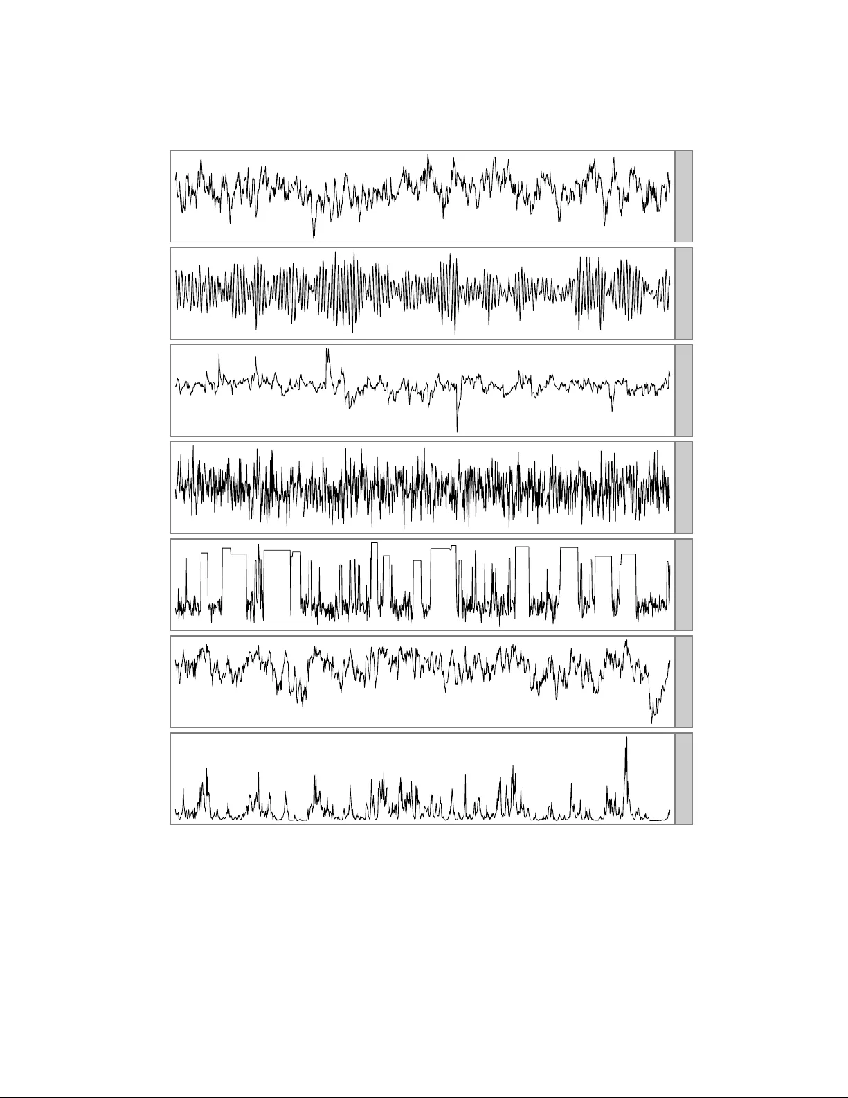
T ec hnical Rep ort No. 1007, Department of Statistics, Univ ersit y of T oron to A Comparison of Metho ds for Computing Auto correlation Time Madeleine B. Thompson m thompson@utstat.toron to.edu h ttp://www.utstat.toron to.edu/m thompson Octob er 29, 2010 Abstract This pap er describ es four metho ds for estimating auto correlation time and ev aluates these metho ds with a test set of seven series. Fitting an autoregressiv e process app ears to b e the most accurate metho d of the four. An R pack age is provided for extending the comparison to more metho ds and test series. 1 In tro duction Auto correlation time measures the con v ergence rate of the sample mean of a function of a stationary , geo- metrically ergo dic Marko v chain with b ounded v ariance. Let { X i } n i =1 b e n v alues of a scalar function of the states of suc h a Mark o v chain, where E X i = µ and v ar X i = σ 2 . Let ¯ X n b e the sample mean of ( X 1 , . . . , X n ). Then, the auto correlation time is the v alue of τ suc h that: r n τ · ¯ X n − µ σ = ⇒ N (0 , 1) (1) Conceptually , the auto correlation time is the n um ber of Marko v chain transitions equiv alent to a single indep enden t draw from the distribution of { X i } . It can b e a useful summary of the efficiency of a Marko v c hain Mon te Carlo (MCMC) sampler. Since there is rarely a closed-form expression for the auto correlation time, man y metho ds for estimating it from the data itself hav e b een developed. This do cument compares four of them: computing batch means, fitting a linear regression to the log sp ectrum, summing an initial sequence of the sample auto correlation function, and mo deling as an autoregressive pro cess. F or a broader con text, tw o classic ov erviews of uncertaint y in MCMC estimation are Gey er (1992) and Neal (1993, § 6.3). The most p opular alternativ e to auto correlation time, p oten tial scale reduction, is dis- cussed b y Gelman and Rubin (1992). 2 Metho ds for computing the auto correlation time 2.1 Batc h means Equation 1 is approximately true for any subsequence, so we can divide the { X i } into batches of size m and compute the sample mean of each batch. As m go es to infinity , the batch means hav e asymptotic v ariance 1 σ 2 · τ /m . So, if s 2 is the sample v ariance of { X i } and s 2 m is the sample v ariance of the batch means, we can estimate the auto correlation time with: ˆ τ n,m = m s 2 m s 2 (2) F or this to b e a consistent estimator of τ , the batch size and the num b er of batches must go to infinity . T o ensure this, I use n 1 / 3 batc hes of size n 2 / 3 . Fishman (1978, § 5.9) discusses batch means in great detail; Neal (1993, p. 104) and Geyer (1992, § 3.2) discuss batch means in the context of MCMC. 2.2 Fitting a linear regression to the log sp ectrum In the sp ectrum fit metho d (Heidelb erger and W elch, 1981, § 2.4), a linear regression is fit to the low er fre- quencies of the log-spectrum of the c hain and used to compute an estimate of the spectrum at frequency zero, whic h we will denote by ˆ I 0 . Let s 2 b e the sample v ariance of the { X i } . W e can estimate the auto correlation time with: ˆ τ = ˆ I 0 s 2 (3) This is implemen ted by the spectrum0 function in R’s CODA pack age (Plummer et al., 2006). First and second order p olynomial fits are practically indistinguishable on the test series describ ed in section 3, so this pap er only explicitly includes the results for a first order fit. 2.3 Initial sequence estimators One form ula for the auto correlation time is (Straatsma et al., 1986, p. 91): τ = 1 + 2 ∞ X k =1 ρ k (4) where ρ k is the auto correlation function (ACF) of the series at lag k . F or small lags, ρ k can b e estimated with: ˆ ρ k = 1 ns 2 n − k X i =1 ( X i − ¯ X n )( X i + k − ¯ X n ) (5) But, this is not defined for lags greater than n − 1, and the partial sum ˆ ρ 1 + · · · + ˆ ρ n − 1 do es not hav e a v ariance that go es to zero as n go es to infinity , so substituting all v alues from equation 5 in to equation 4 is not an acceptable wa y to estimate τ . Gey er (1992) sho ws that, for rev ersible Mark ov c hains, sums of pairs of consecutiv e ACF v alues, ρ i + ρ i +1 , are alwa ys p ositive, so one can obtain a consistent estimator, the initial p ositive sequence (IPS) estimator, b y truncating the sum when the sum of adjacent sample ACF v alues is negative. F urther, the sequence of sums of pairs is alw ays decreasing, so one can smo oth the initial positive sequence when a sum of tw o adjacent sample ACF v alues is larger than the sum of the previous pair; the resulting estimator is the initial monotone sequence (IMS) estimator. Finally , the sequence of sums of pairs is also con vex. Smo othing the sum to account for this results in the initial con vex sequence (ICS) estimator. I was unable to distinguish the b ehavior of the IPS, IMS, and ICS estimators, so the comparisons of this pap er only directly include the ICS estimator. 2 2.4 AR pro cess Another wa y to estimate the auto correlation time, based on CODA’s spectrum0.ar (Plummer et al., 2006), is to mo del the series as an AR( p ) pro cess, with p c hosen b y AIC. W e supp ose a mo del of the form: X t = µ + π 1 X t − 1 + · · · + π p X t − p + a t , a t ∼ N (0 , σ 2 a ) (6) Let ˆ ρ 1: p b e the v ector ( ˆ ρ 1 , . . . , ˆ ρ p ). W e can obtain an estimate the AR coefficients, ˆ π 1: p , with the Y ule–W alker metho d (W ei, 2006, pp. 136–138). Com bining equations 7.1.5 and 12.2.8b of W ei (2006, pp. 137, 274–275), w e can estimate the auto correlation time with: ˆ τ = 1 − ˆ ρ T 1: p ˆ π 1: p  1 − 1 T p ˆ π 1: p  2 (7) Because the Y ule–W alker metho d estimates the asymptotic v ariance of ˆ π 1: p , Monte Carlo simulation can b e used to generate a confidence in terv al for the auto correlation time. F or more information on this metho d, see Fishman (1978, § 5.10) and Thompson (2010). 3 Sev en test series I ev aluate the methods of section 2 with seven series. The first 10,000 elements of eac h are plotted in figure 1. • AR(1) is an AR(1) pro cess with autocorrelation equal to 0 . 98 and uncorrelated errors. Using equa- tion 7, its auto correlation time is 99. It is, in one sense, the simplest p ossible series with an auto cor- relation time other than one. • AR(2) is the AR(2) pro cess with p oles at − 1 + 0 . 1 i and − 1 − 0 . 1 i : Z t = 1 . 98 Z t − 1 − 0 . 99 Z t − 2 + a t , a t ∼ N (0 , 1) (8) Despite oscillating with a p erio d of ab out 60, the terms in its auto correlation function nearly cancel eac h other out, so its auto correlation time is appro ximately tw o. This series is included to iden tify metho ds that cannot identify cancellation in long-range dep endence. • AR(1)-ARCH(1) is an AR(1) pro cess with auto correlation 0 . 98 and auto correlated errors: Z t = 0 . 98 Z t − 1 + a t , a t ∼ N  0 , 0 . 01 + 0 . 99 a 2 t − 1  (9) Its auto correlation time is also 99. This series could confound metho ds that assume constan t step v ariance. • Met-Gauss is a sequence of states generated b y a Metrop olis sampler with Gaussian prop osals sam- pling from a Gaussian probability distribution. It has an auto correlation time of eight. It is a simple example of a state sequence from an MCMC sampler. 3 0 5000 10000 AR(1) AR(2) AR(1)−ARCH(1) Met−Gauss ARMS−Bimodal Stepout−Log−V ar Stepout−V ar Figure 1: The first 10,000 elements of seven series used as a test set. See section 3 for more information. 4 series length autocorrelation time 0.1 1 10 100 0.1 1 10 100 AR(1) i i i i i i i i i i i i i i i a a a a a a a a a a a a a a a s s s s s s s s s s s s s s b b b b b b b b b b b b b b b ARMS−Bimodal i i i i i i i i i i i i i i i a a a a a a a a a a a a a a a s s s s s s s s s s s s s s s b b b b b b b b b b b b b b b 10 100 1,000 10,000 100,000 AR(2) i i i i i i i i i i i i i i i a a a a a a a a a a a a a a a s s s s s s s s s s s s s b b b b b b b b b b b b b b b Stepout−Log−V ar i i i i i i i i i i i i i i i a a a a a a a a a a a a a a a s s s s s s s s s s s s s s s b b b b b b b b b b b b b b b 10 100 1,000 10,000 100,000 AR(1)−ARCH(1) i i i i i i i i i i i i i i i a a a a a a a a a a a a a a a s s s s s s s s s s s s s s s b b b b b b b b b b b b b b b Stepout−V ar i i i i i i i i i i i i i i i a a a a a a a a a a a a a a a s s s s s s s s s s s s s s s b b b b b b b b b b b b b b b 10 100 1,000 10,000 100,000 Met−Gauss i i i i i i i i i i i i i i i a a a a a a a a a a a a a a a s s s s s s s s s s s s s s s b b b b b b b b b b b b b b b 10 100 1,000 10,000 100,000 method i ICS a AR process s Spec. fit b Batch means Figure 2: Autocorrelation times computed b y four metho ds on seven series for a range of subsequence lengths. Each plot symbol represents a single estimate. The dashed line indicates the true autocorrelation time. Breaks in the lines for sp ectrum fit indicate instances where the metho d failed to pro duce an estimate. See section 4 for discussion. • ARMS-Bimo dal is also a sequence of states from an MCMC simulation, ARMS (Gilks et al., 1995) applied to a mixture of tw o Gaussians. The sampler is badly tuned, so it rarely accepts a proposal when near the upp er mo de. It has an auto correlation time of approximately 200. • Step out-Log-V ar is a third MCMC sequence, the log-v ariance parameter of slice sampling with stepping out (Neal, 2003, § 4) sampling from a ten-parameter multilev el mo del (Gelman et al., 2004, pp. 138–145). Its auto correlation time is approximately 200. • Step out-V ar was generated by exponentiating the states of Step out-Log-V ar. Because its sample mean is dominated by large observ ations, its auto correlation time, approximately 100, is not the same as that of Step out-Log-V ar. Like ARMS-Bimo dal and Step out-Log-V ar, it is a challenging, real-world example of a sequence whose auto correlation time might b e unknown. 5 lag −0.5 0.0 0.5 1.0 0 20 40 60 80 100 120 140 Figure 3: The auto correlation function of the AR(2) series. See section 4 for discussion. 4 Comparison of metho ds F or each series, I compare the true auto correlation time to the auto correlation time estimated b y each metho d for subsequences ranging in length from 10 to 500,000. The results are plotted in figure 2. All four metho ds conv erge to the true v alue on all seven chains, with the exception of ICS on the AR(2) pro cess. In general, the AR pro cess metho d conv erges to the true auto correlation time fastest, follo wed by ICS, batch means, and finally sp ectrum fit, which does not ev en pro duce an estimate in all cases. All four metho ds tend to underestimate auto correlation times for all short sequences except those from the AR(2) pro cess, which app ears in small samples to hav e a longer auto correlation time than it actually do es. ICS is inconsisten t on the AR(2) pro cess b ecause the auto correlation function of the AR(2) pro cess is significan t at lags larger than its first zero-crossing (see figure 3). ICS and the other initial sequence estimators are not necessarily consisten t when the underlying chain is not reversible; an AR(2) pro cess is not, when considered a tw o state system. These estimators stop summing the sample auto correlation function the first time its v alues fall b elow zero, so these estimators never see that v alues at large lags cancel v alues at small lags. The AR pro cess metho d can also generate approximate confidence interv als for the auto correlation time. 95% confidence in terv als generated by the AR pro cess metho d are shown in figure 4. The in terv als are somewhat reasonable for subsequences longer than the true auto correlation time. An exception is on AR(2), where the first few hundred elements do not represent the entire series but app ear as though they migh t. 5 Discussion The AR pro cess metho d is more accurate than the three other metho ds and is the only metho d that, as implemen ted, generates confidence interv als, so I usually prefer it to the other three. The batc h m eans estimate is faster to compute and almost as accurate, so it may b e useful when sp eed is imp ortant and confidence in terv als are not necessary . 6 series length autocorrelation time 0.01 0.1 1 10 100 1,000 0.01 0.1 1 10 100 1,000 AR(1) a a a a a a a a a a a a a a a ARMS−Bimodal a a a a a a a a a a a a a a a 10 100 1,000 10,000 100,000 AR(2) a a a a a a a a a a a a a a a Stepout−Log−V ar a a a a a a a a a a a a a a a 10 100 1,000 10,000 100,000 AR(1)−ARCH(1) a a a a a a a a a a a a a a a Stepout−V ar a a a a a a a a a a a a a a a 10 100 1,000 10,000 100,000 Met−Gauss a a a a a a a a a a a a a a a 10 100 1,000 10,000 100,000 Figure 4: AR pro cess-generated p oint estimates and 95% confidence interv als for the auto correlation times of seven series for a range of subsequence lengths. The dashed line indicates the true auto correlation time. The confidence interv als are somewhat reasonable. See section 4 for discussion. 7 The test set only con tains seven series and reflects the type of data I encounter in m y o wn work. T o extend the comparison to other metho ds and series, one can use ACTCompare, an R pack age av ailable at h ttp://www.utstat.toronto.edu/m thompson. 6 Ac knowledgmen ts I would lik e to thank Radford Neal for his comments on this pap er and Charles Geyer for his discussion of initial sequence estimators. References Fishman, G. S. (1978). Principles of Discr ete Event Simulation . John Wiley and Sons. Gelman, A., Carlin, J. B., Stern, H. S., and Rubin, D. B. (2004). Bayesian Data Analysis, Se c ond Edition . Chapman and Hall/CRC. Gelman, A. and Rubin, D. B. (1992). Inference from iterativ e sim ulation using m ultiple sequences. Statistic al Scienc e , (4):457–511. Gey er, C. J. (1992). Practical Marko v Chain Monte Carlo. Statistic al Scienc e , 7(4):473–511. Gilks, W. R., Best, N. G., and T an, K. K. C. (1995). Adaptive rejection Metrop olis sampling within Gibbs sampling. Applie d Statistics , 44(4):455–472. Heidelb erger, P . and W elch, P . D. (1981). A sp ectral metho d for confidence interv al generation and run length con trol in simulations. Communic ations of the ACM , 24(4):233–245. Neal, R. M. (1993). Probabilistic inference using Marko v Chain Monte Carlo metho ds. T echnical Rep ort CR G-TR-93-1, Dept. of Computer Science, Universit y of T oron to. Neal, R. M. (2003). Slice sampling. Annals of Statistics , 31:705–767. Plummer, M., Best, N., Co wles, K., and Vines, K. (2006). CODA: Conv ergence diagnosis and output analysis for MCMC. R News , 6(1):7–11. Straatsma, T. P ., Berendsen, H. J. C., and Stam, A. J. (1986). Estimation of statistical errors in molecular sim ulation calculations. Mole cular Physics , 57(1):89–95. Thompson, M. B. (2010). Graphical comparison of MCMC p erformance. In preparation. W ei, W. W. S. (2006). Time Series Analysis: Univariate and Multivariate Metho ds, Se c ond Edition . Pear- son/Addison W esley . 8