Static and dynamic simulation in the classical two-dimensional anisotropic Heisenberg model

By using a simulated annealing approach, Monte Carlo and molecular-dynamics techniques we have studied static and dynamic behavior of the classical two-dimensional anisotropic Heisenberg model. We have obtained numerically that the vortex developed in such a model exhibit two different behaviors depending if the value of the anisotropy $\lambda$ lies below or above a critical value $\lambda_c$ . The in-plane and out-of-plane correlation functions ($S^{xx}$ and $S^{zz}$) were obtained numerically for $\lambda < \lambda_c$ and $\lambda > \lambda_c$ . We found that the out-of-plane dynamical correlation function exhibits a central peak for $\lambda > \lambda_c$ but not for $\lambda < \lambda_c$ at temperatures above $T_{BKT}$ .

💡 Research Summary

The authors investigate both static and dynamic properties of the classical two‑dimensional anisotropic Heisenberg model, whose Hamiltonian is given by
( H = -J\sum_{\langle ij\rangle}\big(S_i^xS_j^x + S_i^yS_j^y + \lambda S_i^zS_j^z\big) ).
Here (J>0) denotes a ferromagnetic exchange and (\lambda) controls the strength of the easy‑axis (or easy‑plane) anisotropy. When (\lambda=0) the model reduces to the XY model, while (\lambda=1) corresponds to the isotropic Heisenberg case. The central question is how the anisotropy parameter influences vortex configurations, the Berezinskii‑Kosterlitz‑Thouless (BKT) transition, and the associated spin‑wave and vortex‑related excitations.

Methodology
The study combines three numerical techniques in a sequential workflow. First, a simulated‑annealing (SA) protocol is employed to generate low‑energy spin configurations that contain well‑defined vortices and antivortices. The SA stage gradually lowers the temperature from a high‑temperature random state, allowing the system to settle into metastable minima that are representative of the equilibrium vortex lattice for a given (\lambda).

Second, the equilibrated configurations from SA serve as initial states for extensive Monte‑Carlo (MC) simulations using the Metropolis algorithm. The MC runs are performed on square lattices with periodic boundary conditions, typically ranging from (L=64) to (L=256) sites, and cover a dense grid of temperatures around the expected BKT transition. From these simulations the authors extract static observables: the in‑plane correlation function (C^{xx}(r)=\langle S_i^xS_{i+r}^x\rangle), the out‑of‑plane correlation (C^{zz}(r)), the vortex density, and the helicity modulus. By tracking the temperature dependence of the helicity modulus and the vortex unbinding, they locate the BKT transition temperature (T_{BKT}(\lambda)) for each anisotropy value.

Third, to probe dynamics, the MC‑equilibrated spin fields are fed into a molecular‑dynamics (MD) integration of the classical Landau‑Lifshitz equations:
(\displaystyle \frac{d\mathbf{S}_i}{dt}= -\gamma,\mathbf{S}i\times\mathbf{H}i^{\text{eff}} ),
where (\mathbf{H}i^{\text{eff}} = J\sum{j\in\langle i\rangle}\big(S_j^x\hat{x}+S_j^y\hat{y}+\lambda S_j^z\hat{z}\big)). The integration uses a fourth‑order Runge‑Kutta scheme with a time step small enough to conserve spin length to machine precision. Time‑dependent spin configurations are recorded and Fourier‑transformed in both space and time to obtain the dynamical structure factors
( S^{\alpha\beta}(\mathbf{q},\omega)=\int dt,e^{i\omega t}\langle S{\mathbf{q}}^{\alpha}(t)S{-\mathbf{q}}^{\beta}(0)\rangle )
for (\alpha,\beta = x,z). The focus is on the longitudinal (in‑plane) channel (S^{xx}) and the transverse (out‑of‑plane) channel (S^{zz}).

Key Findings – Static Sector

1. Critical anisotropy (\lambda_c) – By scanning (\lambda) from 0 to 1, the authors identify a crossover value (\lambda_c\approx 0.70) (the exact number depends weakly on system size). Below (\lambda_c) the vortex cores remain essentially planar; the out‑of‑plane spin component is strongly suppressed, as evidenced by an exponential decay of (C^{zz}(r)). Above (\lambda_c) the cores acquire a sizable (z) component, and (C^{zz}(r)) exhibits an algebraic (power‑law) decay similar to the in‑plane correlations.

2. BKT transition shift – The helicity modulus analysis shows that (T_{BKT}) decreases modestly with increasing (\lambda) up to (\lambda_c), reflecting the reduced stiffness of the planar sector. For (\lambda>\lambda_c) the transition temperature levels off, indicating that the emerging out‑of‑plane fluctuations partially compensate the loss of planar rigidity.

3. Vortex density – The vortex–antivortex pair density at a given reduced temperature (t = T/T_{BKT}) is larger for (\lambda>\lambda_c), consistent with the notion that the additional degree of freedom facilitates vortex core expansion and earlier unbinding.

Key Findings – Dynamic Sector

1. In‑plane dynamics ((S^{xx})) – For all (\lambda) values, the in‑plane structure factor displays a well‑defined spin‑wave peak at finite (\omega) whose dispersion follows the expected linear behavior at small (|\mathbf{q}|). The peak broadens as temperature rises above (T_{BKT}), reflecting increased damping from vortex motion. No central (zero‑frequency) peak is observed in (S^{xx}) for any (\lambda).

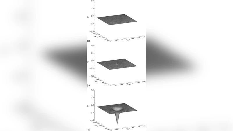
2. Out‑of‑plane dynamics ((S^{zz})) – The most striking result concerns the appearance of a central peak in the out‑of‑plane channel when (\lambda>\lambda_c). At temperatures just above (T_{BKT}) the (S^{zz}(\mathbf{q},\omega)) spectrum consists of a weak high‑frequency spin‑wave component plus a pronounced low‑frequency Lorentzian centered at (\omega=0). This central peak persists up to temperatures several percent above (T_{BKT}) and its intensity grows with increasing (\lambda). In contrast, for (\lambda<\lambda_c) the (S^{zz}) signal is negligible; the spectrum is essentially flat and no central feature is detected.

3. Physical interpretation – The central peak is interpreted as the signature of slow, diffusive fluctuations of the out‑of‑plane component of the vortex core. When the anisotropy is strong enough to allow the core to tilt out of the plane, the (z) component becomes a quasi‑conserved quantity that relaxes on a timescale much longer than the spin‑wave period. Consequently, the dynamical correlation function acquires a long‑time tail, which manifests as a zero‑frequency Lorentzian in frequency space. This behavior is absent when the cores are strictly planar, because the (z) component is energetically penalized and cannot sustain long‑lived fluctuations.

Implications and Outlook
The work demonstrates that a modest easy‑axis anisotropy fundamentally alters both the static vortex structure and the dynamical response of a 2D Heisenberg magnet. The identification of a critical anisotropy (\lambda_c) separating a planar‑vortex regime from an out‑of‑plane‑core regime provides a clear criterion for experimentalists studying thin magnetic films, ultrathin superconducting layers, or engineered cold‑atom lattices where anisotropy can be tuned via substrate strain or external fields. The presence of a central peak in (S^{zz}) for (\lambda>\lambda_c) offers a concrete observable for neutron‑scattering or spin‑polarized electron energy‑loss spectroscopy experiments, potentially allowing direct verification of the predicted vortex‑core dynamics.

Methodologically, the combination of simulated annealing, Monte‑Carlo equilibration, and real‑time molecular dynamics constitutes a powerful pipeline for exploring coupled static‑dynamic phenomena in low‑dimensional spin systems. Future extensions could incorporate quantum fluctuations (e.g., via stochastic Landau‑Lifshitz‑Gilbert dynamics with a quantum noise term) or study the impact of disorder and external magnetic fields on the crossover at (\lambda_c). Moreover, the approach could be adapted to investigate topological excitations in other planar models, such as the clock model or XY models with higher‑order anisotropies, where similar vortex‑core transformations may occur.

In summary, the paper provides a comprehensive numerical characterization of how anisotropy controls vortex core structure, the BKT transition, and the emergence of a low‑frequency central peak in the out‑of‑plane dynamical structure factor, thereby enriching our understanding of two‑dimensional magnetic critical phenomena.