Wind speed vertical distribution at Mt. Graham

The characterization of the wind speed vertical distribution V(h) is fundamental for an astronomical site for many different reasons: (1) the wind speed shear contributes to trigger optical turbulence in the whole troposphere, (2) a few of the astroclimatic parameters such as the wavefront coherence time (tau_0) depends directly on V(h), (3) the equivalent velocity V_0, controlling the frequency at which the adaptive optics systems have to run to work properly, depends on the vertical distribution of the wind speed and optical turbulence. Also, a too strong wind speed near the ground can introduce vibrations in the telescope structures. The wind speed at a precise pressure (200 hPa) has frequently been used to retrieve indications concerning the tau_0 and the frequency limits imposed to all instrumentation based on adaptive optics systems, but more recently it has been proved that V_200 (wind speed at 200 hPa) alone is not sufficient to provide exhaustive elements concerning this topic and that the vertical distribution of the wind speed is necessary. In this paper a complete characterization of the vertical distribution of wind speed strength is done above Mt.Graham (Arizona, US), site of the Large Binocular Telescope. We provide a climatological study extended over 10 years using the operational analyses from the European Centre for Medium-Range Weather Forecasts (ECMWF), we prove that this is representative of the wind speed vertical distribution at Mt. Graham with exception of the boundary layer and we prove that a mesoscale model can provide reliable nightly estimates of V(h) above this astronomical site from the ground up to the top of the atmosphere (~ 20 km).

💡 Research Summary

The paper presents a comprehensive investigation of the vertical wind‑speed profile V(h) above Mt. Graham, Arizona, the site of the Large Binocular Telescope (LBT). Recognizing that wind‑shear drives optical turbulence throughout the troposphere and that key adaptive‑optics (AO) metrics—wave‑front coherence time (τ₀) and equivalent wind speed (V₀)—depend directly on the integral of V(h) weighted by the turbulence strength Cₙ²(z), the authors set out to characterize V(h) on both climatological and operational timescales.

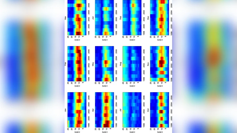
First, a ten‑year climatology (2005‑2014) is built from the European Centre for Medium‑Range Weather Forecasts (ECMWF) operational analyses. These analyses, assimilating a global network of surface observations, radiosondes, and satellite radiances, provide wind data from the surface to ~20 km at a 0.25° (~30 km) horizontal resolution every six hours. By averaging these data month‑by‑month and season‑by‑season, the authors obtain a robust picture of the mean wind structure: a relatively stable wind field above ~2 km, a pronounced jet stream centered at 10‑12 km with speeds of 30‑35 m s⁻¹, and marked seasonal differences—stronger mid‑tropospheric winds in winter that reduce τ₀, and weaker winds in summer that allow AO systems to operate at lower temporal frequencies.

However, the ECMWF products show systematic deficiencies in the boundary layer (≤1 km). The coarse vertical resolution and limited surface observations lead to an under‑estimation of near‑surface wind speeds, which are critical for both telescope vibration control and the low‑altitude contribution to τ₀. To address this gap, the authors employ a high‑resolution mesoscale model (Meso‑Nh). The model is initialized and forced at its lateral boundaries with the ECMWF analyses, runs on a 3 km parent grid with nested domains down to ~0.5 km, and produces 12‑hour forecasts centered on the nightly observing window (00 UTC).

Model validation against on‑site radiosonde launches and ground‑based anemometers demonstrates that the mesoscale simulations capture the boundary‑layer wind structure with a mean absolute error of 1‑2 m s⁻¹, substantially better than the ECMWF analyses. Above the boundary layer, the mesoscale model agrees closely with ECMWF, confirming that the latter remains reliable for the free troposphere.

Using the combined wind profiles, the authors compute τ₀ and V₀ through the standard integrals:

\