Necessary and Sufficient Conditions on Sparsity Pattern Recovery
The problem of detecting the sparsity pattern of a k-sparse vector in R^n from m random noisy measurements is of interest in many areas such as system identification, denoising, pattern recognition, and compressed sensing. This paper addresses the sc…
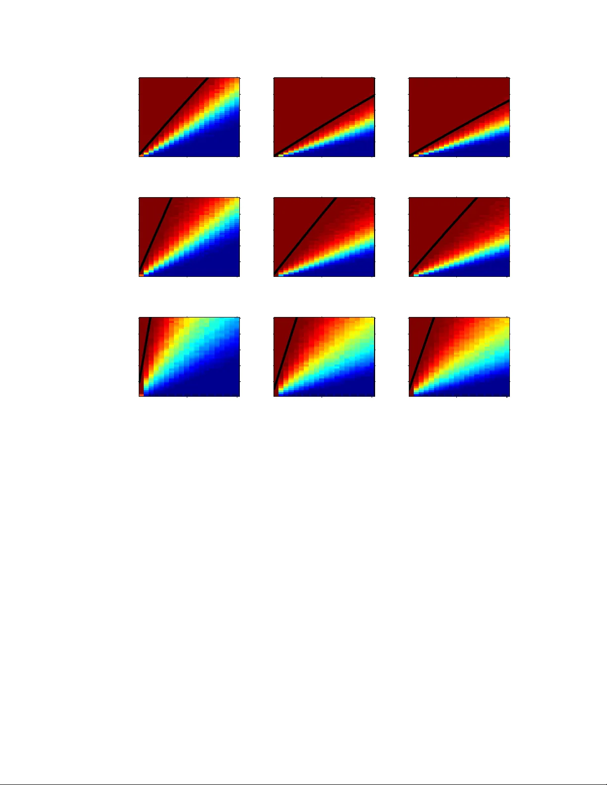
Authors: Alyson K. Fletcher, Sundeep Rangan, Vivek K. Goyal
NECESSAR Y AND SUFFICIENT CONDITIONS FOR SP ARSITY P A TTERN RECO VER Y 1 Necessary and Suf ficient Conditions on Sparsity P attern Reco v ery Alyson K. Fletcher , Member , IEEE, Sundeep Rangan, and V i vek K Goyal, Senior Member , IEEE Abstract The pro blem of detectin g the sparsity pa ttern of a k - sparse vector in R n from m r andom noisy measuremen ts is of interest in m any areas such as sy stem identificatio n, denoising, pattern reco gnition, and com pressed sensing. This paper ad dresses the scaling o f the num ber of measurem ents m , with signal dimension n and sparsity-level nonze ros k , for asymptotically-reliable d etection. W e show a necessary condition f or perfect re covery at any giv en SNR for all algo rithms, regardless of complexity , is m = Ω( k log( n − k )) m easurements. Con versely , it is shown that this scaling of Ω( k log( n − k )) m easurements is sufficient f or a remark ably simple “maximum co rrelation” estimator . Hence this scaling is optima l an d does n ot requir e m ore sop histicated techniq ues such a s lasso or m atching pu rsuit. The constants for both the necessary and sufficient con ditions are precisely defin ed in terms of the m inimum-to - av erag e ratio of th e n onzero comp onents and the SNR. The nece ssary condition improves u pon pr evious resu lts for m aximum likelihoo d estimation. For lasso, it also provides a nece ssary con dition at any SNR and for low SNR improves upon previous work. The sufficient co ndition p rovides the first asymp totically-reliable detectio n gu arantee at finite SNR. Index T erms compressed sensing, conv ex op timization, lasso, ma ximum likelihoo d estimation, r andom matrices, random projection s, regression, sparse approx imation, sparsity , sub set selection I . I N T R O D U C T I O N Suppose one is given an observation y ∈ R m that was generated through y = Ax + d , wh ere A ∈ R m × n is known and d ∈ R m is an additiv e n oise vector with a kno wn d istribution. It may be desirable for an estimate of x to ha ve a small n umber of nonzer o components. An intu itiv e example is when one wants to choose a small subset from a large number of possibl y-related factors that linearly influence a vector of observed da ta. Each factor corre spon ds to a col umn of A , and o ne wishes to find a sm all subset of columns with which to form a li near combination that clo sely matches the o bserved data y . This is t he subset s election problem in (linear) regression [1], and it give s no reason to penalize large values for the nonzero compo nents. In this paper , we assume that the true signal x has k nonzero entries and that k is known when estimating x from y . W e are concerned with establish ing necessary and sufficient conditi ons for the recovery of th e positions of the nonzero entries of x , which we call the sparsity pat tern . On ce the sparsity pattern is correct, n − k colu mns of A can be ignored and the stabili ty of the solution is well understood; howe ver , we do not stu dy any other performance criterion. This work was supported in part by a U ni versity of California P resident’ s P ostdoctoral Fell o wship, NSF CARE ER Grant CCF- 64383 6, and t he C entre Bernoulli at ´ Ecole Polytechnique F ´ ed ´ erale de Lausanne. A. K. Fletcher (email: alyson@eecs.berk eley .edu) is wit h the Department of El ectrical E ngineering and Computer S ciences, Unive rsity of California, Berkele y . S. Rangan (email: srangan@qualcomm.com) is with Qualcomm T echnolo gies, Bedminster , NJ. V . K. G oy al (email: vgoyal@mit.edu) is wit h the Department of El ectrical Engineering and Computer Science and the R esearch Laboratory of El ectronics, Massachusetts Institute of T echnology . 2 NECESSAR Y AN D SUFFICIENT CONDITIONS FOR SP ARSITY P A TT ERN RE CO VER Y A. Pr evious W ork Sparsity pattern recov ery (or more simply , sparsity rec overy) has recei ved considerable attention in a var iety guises. Mo st t ransparent from our formulation is the connection to sparse approximati on. In a typical sparse approximati on problem, one i s given data y ∈ R m , d ictionary 1 A ∈ R m × n , and tolerance ǫ > 0 . The aim is to find ˆ x with the fewest number of nonzero entries among those satisfying k A ˆ x − y k ≤ ǫ . This prob lem is NP-hard [3] but greedy heuris tics (matching p ursuit [2] and i ts variants) and con vex relaxations (basis p ursuit [4], lasso [5] and others) can b e eff ective under certain conditions on A and y [6]–[8]. Scaling laws for sp arsity recov ery wi th any A were first given in [9]. More recently , the concept of “sensing” sparse x th rough multi plication by a su itable random matrix A , with measurement error d , has been termed compr essed sensing [1 0]–[12]. This has popularized t he study of sparse approximation wit h respect to random di ctionaries, which was considered also in [13]. Result s are generally phrased as the asym ptotic scaling of the numb er of measurements m (the length of y ) needed for s parsity recovery to succeed wi th high p robability , as a function of the other problem p arameters. Mo re specifically , m ost results are su f ficient conditions for specific tractable recovery algori thms t o su cceed. For example, if A has i.i.d. Gaussian entries and d = 0 , then m ≍ 2 k log( n/ k ) dictates the minim um scaling at w hich b asis pursuit succeeds with high probability [ 14]. W ith non zero nois e variance, necessary and suffi cient con ditions for t he success of lasso in this setting hav e the asymptot ic scalin g [15] m ≍ 2 k log ( n − k ) + k + 1 . (1) T o understand the ultim ate l imits of sparsity recov ery , while als o casting light on th e effic acy of lass o or o rthogonal matching pu rsuit (OMP), it is of interest to deter mi ne necessary and suf ficient cond itions for an optimal recovery algorith m t o succeed. Of course, since it is sufficient for lasso, the conditio n (1) is suffic ient for an optim al algorithm. Is it close to a necessary condition? W e address precisely this question by proving a nec essary condition that differs from (1) by a factor that is constant with r espect to n and k whi le dependi ng on the signal-to-noi se ratio (SNR) and mean-to-ave rage ratio (MAR), which will be defined precisely in Section II. Furthermore, we present an extremely si mple algorithm for which a sufficient condition for sparsity recovery i s simil arly wit hin a cons tant factor of (1). Pre vious necessary conditions had been based on informatio n-theoretic analyses such as the capacity ar gument s in [16], [17] and a use of F ano’ s in equality i n [18]. M ore recent publ ications w ith necessary conditions i nclude [19]–[22]. As described in Section III, our new necessary cond itions are stronger than the previous results. T abl e I pre vie ws our m ain results and places (1) in context. The measurement model a nd parameters MAR and SNR are defined in th e following section. Arbitrarily small constants have been omitted, and the last column—labeled sim ply SNR → ∞ —is m ore specifically for MAR > ǫ > 0 for som e fixed ǫ and SNR = Ω( k ) . B. P a per Or ganizatio n The setting is formalized in Section II. In particular , we define our concepts of signal-to-noi se ratio and mean-to-av erage ratio; our result s clarify th e roles of these quanti ties in the sparsity recov ery problem. Necessary conditions for s uccess of any alg orithm are consi dered in Section III. There we present a new necessary condi tion and compare it t o previous results and numerical experiments. Section IV introduces a very s imple recov ery algorithm for the p urpose of showing that a s uf ficient condi tion for it s success is rather weak—it has the same dependence on n and k as (1). Conclusions are given in Section V, and proofs appear in the Appendix. 1 The term seems to have originated in [2] and may apply to A or the columns of A as a set. FLETCHER, RANGAN AND GOY AL 3 finite SNR SNR → ∞ Any algorithm must fail m < 2 MAR · SNR k log ( n − k ) + k − 1 m ≤ k Theorem 1 (elementary) Necessary and unkno wn (expressions abov e m ≍ 2 k log( n − k ) + k + 1 suf ficient for lasso and ri ght are necessary) W ainwright [15] Sufficient for maximum m > 8(1+ SNR ) MAR · SNR k log ( n − k ) m > 8 MAR k log ( n − k ) correlation estimator (8 ) Theorem 2 from Theorem 2 T ABLE I S U M M A RY O F R E S U LT S O N M E A S U R E M E N T S C A L I N G F O R R E L I A B L E S PA R S I T Y R E C OV E RY ( S E E B O DY F O R D E FI N I T I O N S A N D T E C H N I C A L L I M I TA T I O N S ) I I . P RO B L E M S T A T E M E N T Consider estimatin g a k -sparse vector x ∈ R n through a vector o f observations, y = Ax + d , (2) where A ∈ R m × n is a random matrix with i.i.d. N (0 , 1 /m ) entries and d ∈ R m is i.i. d. unit-variance Gaussian n oise. Denote t he s parsity pat tern o f x (positions of nonzero entries) by the set I true , which i s a k -element subs et of the set of indices { 1 , 2 , . . . , n } . Estim ates of th e sp arsity patt ern will be denoted by ˆ I with subscripts i ndicating the ty pe of estim ator . W e seek conditions under which there exists an estimator such that ˆ I = I true with high probability . In addition to the signal di mensions, m , n and k , we will show that there are two variables that dictate the ability to d etect t he sparsity pattern reliably: t he SNR, and what we wi ll call the minimum-to-average ratio . The SNR i s defined by SNR = E [ k Ax k 2 ] E [ k d k 2 ] = E [ k Ax k 2 ] m . (3) Since we are considering x as an unknown deterministic vector , the SNR can be further simplified as follows: The entries of A are i.i.d. N (0 , 1 /m ) , so columns a i ∈ R m and a j ∈ R m of A s atisfy E [ a ′ i a j ] = δ ij . Therefore, the signal energy is given by E k Ax k 2 = E " k X j ∈ I true a j x j k 2 # = X X i,j ∈ I true E [ a ′ i a j x i x j ] = X X i,j ∈ I true x i x j δ ij = k x k 2 . Substitutin g in to the definition (3), the SNR is g iv en by SNR = 1 m k x k 2 . (4) The minim um-to-av erage ratio of x is d efined as MAR = min j ∈ I true | x j | 2 k x k 2 /k . (5) Since k x k 2 /k is the ave rage of {| x j | 2 | j ∈ I true } , MAR ∈ (0 , 1] with the upper limit occurring when all the non zero entries of x have the same m agnitude. 4 NECESSAR Y AN D SUFFICIENT CONDITIONS FOR SP ARSITY P A TT ERN RE CO VER Y Remarks: Other works u se a variety of norm alizations, e.g.: the entries of A have variance 1 /n i n [12], [20]; the entries of A ha ve unit variance and t he va riance of d is a variable σ 2 in [15], [18], [21], [22]; and ou r scaling of A and a noise var iance of σ 2 are used i n [23 ]. This necessit ates g reat care in comp aring results. Some results inv olve MAR · SNR = k m min j ∈ I true | x j | 2 . While a sim ilar quantity af fects a regularization weight sequence in [15 ], there it does no t affec t the number of measurement s required for the success of lasso. 2 The magnit ude of the s mallest nonzero entry of x is also prominent in the phrasing of results in [21], [22]. I I I . N E C E S S A RY C O N D I T I O N F O R S PA R S I T Y R E C OV E RY W e first consider sparsity recove ry without being con cerned wit h comput ational complexity o f the estimation algorithm. Since th e vector x ∈ R n is k -sparse, the vector Ax belongs to one of L = n k subspaces spanned by k of the n colum ns of A . Estim ation of the s parsity pattern is the selection of one of these subspaces, and since the nois e d is Gaussian, the probabil ity of error is minimi zed by choosing the sub space closest to the observed vector y . Thi s results in the maxi mum likelihood (ML) est imate. Mathematically , the ML estim ator can be described as foll ows. Given a subset J ⊆ { 1 , 2 , . . . , n } , let P J y denote the orthogonal projectio n o f the vector y onto the subspace spanned by the vectors { a j | j ∈ J } . The ML estimate of the sparsity p attern is ˆ I ML = arg max J : | J | = k k P J y k 2 , where | J | deno tes t he cardinalit y of J . That is, the ML estimate is th e set of k indices such th at the subspace sp anned by the corresponding colum ns o f A con tain the maximum signal ener gy of y . Since the number of subspaces, L , grows exponentiall y in n and k , an e xhaustive search is com puta- tionally infeasible. Ho wever , the p erformance of M L estimation provides a lower boun d on the number of measurements needed by any algorithm that cannot exploit a pri ori information on x other than it being k -sparse. Theor em 1: Let k = k ( n ) and m = m ( n ) vary with n such that lim n →∞ k ( n ) = ∞ and m ( n ) < 2 − δ MAR · SNR k log( n − k ) + k − 1 (6) for some δ > 0 . Then e ven the ML estimator asymp totically cannot detect the sp arsity pattern, i.e., lim n →∞ Pr ˆ I ML = I true = 0 . Pr oof: See Appendix B. The theorem shows that for fixed SNR and MAR , t he scaling m = Ω( k log ( n − k )) is necessary for reliable sparsity pattern r ecovery . The ne xt section will sho w that this scaling ca n be achiev ed with an extremely simple method. Remarks: 1) The theorem applies for any k ( n ) such that lim n →∞ k ( n ) = ∞ , in cluding both cases with k = o ( n ) and k = Θ( n ) . In particular , under l inear sparsity ( k = α n for some constant α ), the theorem shows that m ≍ 2 α MAR · SNR n log n measurements are necessary for sparsity recov ery . Simi larly , i f m/n is bounded above by a constant, then sp arsity recovery will certainly fail unless k = O ( n/ log n ) . 2 The formulation of [15] makes SNR = Θ( n ) , which obscures the effec t of the noise lev el. See also the second remark following Theorem 2. FLETCHER, RANGAN AND GOY AL 5 2) In the case o f MAR · SNR < 1 , the bound (6) improves upon the necessary condi tion of [15] for the asymptotic s uccess of lasso by th e factor ( MAR · SNR ) − 1 . 3) The bound (6) can be compared against t he inform ation-theoretic bounds mentioned earlier . The tightest o f these bound s is in [17 ] and shows th at the problem d imensions must satisfy 2 m log 2 n k ≤ log 2 (1 + SNR ) − α log 2 (1 + SNR α ) , (7) where α = k /n is th e sparsity ratio . For large n and k , the boun d can be rearranged as m ≥ 2 h ( α ) α log 2 (1 + SNR ) − α log 2 (1 + SNR α ) − 1 k , where h ( · ) i s the binary entropy function. In p articular , w hen the sparsity ratio α is fixed, the bo und shows only that m nee ds to gro w at l east linearly with k . I n contrast , T heorem 1 shows that with fixed sparsity ratio m = Ω( k lo g( n − k )) is necessary for reli able sparsity recov ery . Thus, the bound in Theorem 1 is s ignificantly t ighter a nd re veals t hat t he previous inform ation-theoretic necessary conditions from [16]–[18], [21], [22] are overly opti mistic. 4) Results more sim ilar to Theorem 1—based on direct analys es of error ev ents rather than informatio n- theoretic ar guments—app eared in [19], [20]. The pre vious re sul ts sho wed that with fi xed SNR as defined here, sparsity recovery wit h m = Θ( k ) mus t fail. The more re fined analysis in this p aper giv es the add itional log ( n − k ) factor and the precise dependence on MAR · SNR . 5) Theorem 1 is not contradicted by the rele vant sufficient condi tion of [21], [22]. That sufficient condition hold s for scaling t hat g iv es l inear sparsit y and MAR · SNR = Ω( √ n log n ) . For MAR · SNR = √ n log n , Theorem 1 shows that fewer t han m ≍ 2 √ k log k measurements will cause M L decoding to fail, while [22, Th m. 3.1] shows that a typicalit y-based decoder will succeed wit h m = Θ( k ) measurements. 6) Not e that the necessary condition of [18] is pro ven for MAR = 1 . Theorem 1 gi ves a bou nd that increases for small er MAR ; this suggests (tho ugh does not prove, since the cond ition is merely necessary) t hat smaller MAR makes the p roblem harder . Numerical validation: Computational confirmation of Theorem 1 is technically impossible, and ev en qualitative support is ha rd to obtain because of t he high compl exity of ML detection. Nevertheless, we may obtain s ome evidence through Mont e Carlo simul ation. Fig. 1 shows the probabilit y of success of ML d etection for n = 20 as k , m , SNR , and MAR are varied, with each point representi ng at least 500 independent trials. Each subpanel giv es simulation re sul ts for k ∈ { 1 , 2 , . . . , 5 } and m ∈ { 1 , 2 , . . . , 40 } for one ( SNR , MAR ) pai r . Signals with MAR < 1 are created by ha ving one small nonzero compon ent and k − 1 equal, larger no nzero components. Overlaid on the color-intensity pl ots is a black curve representing (6). T aki ng any on e column of one su bpanel from bottom to top shows that as m is increased, there is a transit ion from M L failing t o ML succeeding. On e can see that (6) fol lows the failure-success transition qualitati vely . In particular , the empirical dependence on SNR and MA R approximately follows (6). Em pirically , for the (sm all) value of n = 20 , it s eems t hat wi th MAR · SNR held fixed, sparsity recovery becomes easier as SNR increases (and MAR decreases). Less extensive Monte Carlo sim ulations for n = 40 are reported in Fig. 2. The resul ts are qualitatively similar . As might be expected, th e transit ion from lo w to hi gh prob ability of successful recov ery as a function of m appears more sharp at n = 40 than at n = 20 . I V . S U FFI C I E N T C O N D I T I O N W I T H M A X I M U M C O R R E L A T I O N D E T E C T I O N Consider the following simpl e estim ator . As before, l et a j be the j th column of the random matrix A . Define the maximum corr elation (MC) estimate as ˆ I MC = j : | a ′ j y | is one of t he k lar gest values of | a ′ i y | . (8) 6 NECESSAR Y AN D SUFFICIENT CONDITIONS FOR SP ARSITY P A TT ERN RE CO VER Y (1, 1) 2 4 5 10 15 20 25 30 35 40 (2, 1) 2 4 5 10 15 20 25 30 35 40 (5, 1) 2 4 5 10 15 20 25 30 35 40 (10, 1) 2 4 5 10 15 20 25 30 35 40 (10, 0.5) 2 4 5 10 15 20 25 30 35 40 (10, 0.2) 2 4 5 10 15 20 25 30 35 40 (10, 0.1) 2 4 5 10 15 20 25 30 35 40 0 0.2 0.4 0.6 0.8 1 P S f r a g r e p l a c e m e n t s k k k k k k k m Fig. 1. Simulated success probability of ML detection for n = 20 and many values of k , m , SNR , and MAR . Each subfigure giv es simulation results for k ∈ { 1 , 2 , . . . , 5 } and m ∈ { 1 , 2 , . . . , 40 } for one ( SNR , MAR ) pair . Each subfigure heading gives ( SNR , MAR ) . Each point represents at l east 500 independent trial s. Overlaid on the color-intensity plots is a black curve representing (6 ). (10, 1) 2 4 10 20 30 40 (10, 0.5) 2 4 10 20 30 40 P S f r a g r e p l a c e m e n t s k k m Fig. 2. Simulated success probability of ML detection for n = 40 ; SNR = 10 ; MAR = 1 (left) or MAR = 0 . 5 (r ight); and many v alues of k and m . Each subfigure giv es simulation results for k ∈ { 1 , 2 , . . . , 5 } and m ∈ { 1 , 2 , . . . , 40 } , w ith each point representing at least 1000 independe nt trials. Overlaid on the color-intensity plots (wit h scale as in Fig. 1) is a black curve r epresenting (6). This algori thm si mply correlates the o bserved signal y with all the frame vectors a j and s elects t he ind ices j with the hi ghest correlation. It is significantly s impler than both lasso and matching pursu it and is not meant to be proposed as a com petitive alternative. Rather , t he MC m ethod is int roduced and analyzed to illustrate th at a trivial m ethod can o btain optim al scali ng with respect to n and k . Theor em 2: Let k = k ( n ) and m = m ( n ) v ary with n such that lim n →∞ k = ∞ , lim sup n →∞ k /n ≤ 1 / 2 , and m > (8 + δ )( 1 + SNR ) MAR · SNR k log( n − k ) (9) for so me δ > 0 . Then the m aximum correlation estimato r asymptot ically detects the sparsity pattern, i.e., lim n →∞ Pr ˆ I MC = I true = 1 . Pr oof: See Appendix C. FLETCHER, RANGAN AND GOY AL 7 Remarks: 1) Comparing (6) and (9), we see t hat for a fixed SNR and m inimum-to-average ratio, the simpl e MC estimator needs only a constant factor m ore measurement s than the optim al ML estimato r . In particular , the results show that the scalin g of the minimum number of measurements m = Θ( k log ( n − k )) is both necessary and sufficient. Moreover , t he optim al scaling factor not only does not require ML estimat ion, it does not even require lasso or matching pursuit —it can be achieved with a remarkably sim ply method such as maxim um correlation. There is , of course, a difference in the constant factors of t he expressions (6) and (9). Specifically , the MC method requi res a factor 4(1 + SNR ) more m easurements than ML detection. In particular , for low SNRs (i.e. SNR ≪ 1 ), the factor reduces t o 4. 2) For hi gh SNRs, the gap between t he MC estim ator and the ML esti mator can be large. In particular , the lower bound on the num ber of measurement s requi red by ML decreases t o k − 1 as SNR → ∞ . 3 In contrast, with the MC estim ator increasing the SNR has d iminishin g returns : as SNR → ∞ , the bound on the numb er of m easurements in (9) approaches m > 8 MAR k log( n − k ) . (10) Thus, even with SNR → ∞ , t he mi nimum number of measurements is not improved from m = O ( k log( n − k )) . This dim inishing returns for improved SNR exhibit ed by the MC method is also a probl em for more sophisticated methods such as lasso. For e xample, the analys is of [15] shows that when the SNR = Θ( n ) (so SNR → ∞ ) and MAR is b ounded strictly away from zero, lasso requires m > 2 k log ( n − k ) + k + 1 (11) for reliabl e recover y . Therefore, like t he MC met hod, lasso d oes not ac hieve a scaling better than m = O ( k log( n − k )) , e ven at infinite SNR. 3) There is certainly a gap between MC and lasso. Comparing (10) and (11), we see that, at high SNR, the simple MC method re quires a f actor of at m ost 4 / MAR mo re measurements than lasso. This factor is largest when MAR i s small, which occurs wh en there are relatively s mall non-zero components. Thus, in the high SNR regime, the main benefit of lasso is not that it achiev es an optimal scaling with respect to k and n (whi ch can be a chieved wi th the sim pler MC), but rather that l asso is able to detect small coefficients, e ven when t hey are much b elow the avera ge power . Numerical valida tion: MC sp arsity pattern detection is extremely simple and can thus be si mulated easily for large problem sizes. Fig. 3 reports the resul ts of a l ar ge number Monte Carlo sim ulations of t he MC m ethod wit h n = 100 . T he thresho ld predicted by (9) matches well to the parameter com binations where the probability of success drops below about 0.995. V . C O N C L U S I O N S W e have considered th e problem of detecting t he sparsity pattern of a sparse vector from noisy random linear measurement s. O ur main con clusions are: • Necessary and sufficient scaling with r espect t o n and k . For a given SNR and m inimum-t o-a verage ratio, the scaling of the number of measurements m = O ( k log( n − k )) is both necessary and sufficient for asym ptotically reliable s parsity pattern detection. This scaling is significantly worse than predict ed by previous informatio n-theoretic b ounds. 3 Of course, at least k + 1 measurements are necessary . 8 NECESSAR Y AN D SUFFICIENT CONDITIONS FOR SP ARSITY P A TT ERN RE CO VER Y (1, 1) 10 20 200 400 600 800 1000 (10, 1) 10 20 200 400 600 800 1000 (100, 1) 10 20 200 400 600 800 1000 (1, 0.5) 10 20 200 400 600 800 1000 (10, 0.5) 10 20 200 400 600 800 1000 (100, 0.5) 10 20 200 400 600 800 1000 (1, 0.2) 10 20 200 400 600 800 1000 (10, 0.2) 10 20 200 400 600 800 1000 (100, 0.2) 10 20 200 400 600 800 1000 P S f r a g r e p l a c e m e n t s k k k m m m Fig. 3. Simulated success probability of MC detection for n = 100 and many values of k , m , SNR , and MAR . E ach subfigure gives simulation results for k ∈ { 1 , 2 , . . . , 20 } and m ∈ { 25 , 50 , . . . , 1000 } for one ( SNR , MAR ) pair . Each subfigure heading gives ( SNR , MAR ) , so SNR = 1 , 10 , 100 for the three columns and MAR = 1 , 0 . 5 , 0 . 2 for the three rows. E ach point represents 1000 independent tri als. Overlaid on the color-intensity plots ( with scale as in Fig. 1) is a black curve representing (9). • Scaling optimali ty of a trivia l meth od. The optim al scaling wi th respect to k and n can be achieved with a trivial maximum correlation (MC) m ethod. In particular , bo th lasso and OMP , while likely to do better , are not n ecessary to achieve this scaling. • Dependence on SNR. While the threshold number of measurements for ML and M C sparsi ty recovery to be su ccessful have t he same dependence on n and k , the dependence on SNR differs significantly . Specifically , the MC method requi res a factor of up to 4(1 + SNR ) more measurements than ML. Moreover , as SNR → ∞ , the nu mber of measurements required by ML m ay be as low as m = k + 1 . In contrast, even letting SNR → ∞ , the maximum correlation method still requires a scaling m = O ( k log( n − k )) . • Lasso and dependence on MAR. MC can also be compared to lasso, at least in the high SNR regime. There is a potential gap between MC a nd l asso, b ut the gap is smaller than the gap to ML. Specifica lly , in the high SNR regime, MC requires at m ost 4 / MAR more measurements than lasso, where MAR is the mean-to-avera ge ratio defined in (5). B oth lasso and MC scale as m = O ( k log( n − k )) . Thus, the benefit of lasso is not i n it s scaling with respect to the p roblem dimensio ns, but rather its ability to detect the sparsity pattern even in the presence of relati vely small nonzero coef ficients ( i.e. low MAR ). FLETCHER, RANGAN AND GOY AL 9 While our result s settl e the question of t he optim al scaling of the number o f m easurements m in terms of k and n , there is clearly a gap in the necessary and suffi cient condit ions in terms of the scaling of the SNR. W e hav e seen th at full ML esti mation coul d potentiall y have a scaling in SNR as sm all as m = O ( 1 / SNR ) + k − 1 . An open question is whether there i s any practical algorithm that can achiev e a similar scalin g. A second open issue is to deter mi ne con ditions for partial sparsity recovery . The above result s define conditions for recovering all t he posi tions in the sparsity pattern. H o wever , in many practical appli cations, obtaining some large fraction of these positi ons would be su f ficient. Neither the li mits o f partial sparsity recov ery nor the performance of practical algorithms are compl etely understoo d, t hough som e resul ts have been reported in [20]–[22], [24]. A P P E N D I X A. Deterministic Necessary Condi tion The proof of Theorem 1 is based o n the following d eterministic nece ssary condition for sparsit y recovery . Recall the notatio n that for any J ⊆ { 1 , 2 , . . . , n } , P J denotes the orthogo nal projection onto t he sp an of the vectors { a j } j ∈ J . Addition ally , l et P ⊥ J = I − P J denote the orthog onal p rojection onto the orthogonal complement of span ( { a j } j ∈ J ) . Lemma 1: A necessary conditi on for ML detectio n to s ucceed (i.e. ˆ I ML = I true ) is: for all i ∈ I true and j 6∈ I true , | a ′ i P ⊥ K y | 2 a ′ i P ⊥ K a i ≥ | a ′ j P ⊥ K y | 2 a ′ j P ⊥ K a j (12) where K = I true \ { i } . Pr oof: Note that y = P K y + P ⊥ K y is an o rthogonal decompositi on o f y into the porti ons inside and outside t he sub space S = span( { a j } j ∈ K ) . A n approxi mation of y i n su bspace S leav es residual P ⊥ K y . Intuitively , the condition (12) requires that the residual be at least as h ighly correlated wi th th e remai ning “correct” vector a i as it is wi th any of the “incorrect” vectors { a j } j 6∈ I true . Fix any i ∈ I true , j 6∈ I true and let J = K ∪ { j } = ( I true \ { i } ) ∪ { j } . That is, J is equal to the true sparsity pattern I true , except that a single “correct” i ndex i has been replaced by an “incorrect” i ndex j . If the M L estimator is t o select ˆ I ML = I true then t he energy of the noisy vector y must be larger on the true subs pace I true , than the incorrect subspace J . Therefore, k P I true y k 2 ≥ k P J y k 2 . (13) Now , a simpl e appli cation of t he matrix in version lemma shows that sin ce I true = K ∪ { i } , k P I true y k 2 = k P K y k 2 + | a ′ i P ⊥ K y | 2 a ′ i P ⊥ K a i . (14a) Also, since J = K ∪ { j } , k P J y k 2 = k P K y k 2 + | a ′ j P ⊥ K y | 2 a ′ j P ⊥ K a j . (14b) Substitutin g (14a)–(14b) into (13) and cancelling k P K y k 2 shows (12). 10 NECESSAR Y AND SUFFICIENT CONDITIONS FOR SP ARSITY P A TTE RN RECOVER Y B. Pr oof of Theor em 1 T o sim plify notation, ass ume wit hout loss of generality that I true = { 1 , 2 , . . . , k } . Als o, assum e that t he minimizati on in (5) occurs at j = 1 with | x 1 | 2 = m k SNR · MAR . (15) Finally , since adding measurement s (i.e. increasing m ) c an only improve the chances that ML detection will work, we can assume that in additio n to satisfyi ng (6), the numbers of measurements satisfy the lower bound m > ǫk log( n − k ) + k − 1 , (16) for some ǫ > 0 . This assumptio n i mplies that lim log( n − k ) m − k + 1 = lim 1 ǫk = 0 . (17) Here and in the remain der of t he proof the l imits are as m , n and k → ∞ subject to (6) and (16). W ith these requirement s on m , w e need t o show lim Pr ( ˆ I ML = I true ) = 0 . From Lemma 1, ˆ I ML = I true implies (12). Thus Pr ˆ I ML = I true ≤ Pr | a ′ i P ⊥ K y | 2 a ′ i P ⊥ K a i ≥ | a ′ j P ⊥ K y | 2 a ′ j P ⊥ K a j ∀ i ∈ I true , j 6∈ I true ! ≤ Pr | a ′ 1 P ⊥ K y | 2 a ′ 1 P ⊥ K a 1 ≥ | a ′ j P ⊥ K y | 2 a ′ j P ⊥ K a j ∀ j 6∈ I true ! = Pr(∆ − ≥ ∆ + ) , where ∆ − = 1 log( n − k ) | a ′ 1 P ⊥ K y | 2 a ′ 1 P ⊥ K a 1 , ∆ + = 1 log( n − k ) max j ∈{ k +1 ,. ..,n } | a ′ j P ⊥ K y | 2 a ′ j P ⊥ K a j , and K = I true \ { 1 } = { 2 , . . . , k } . The − and + sup erscripts are used to reflect that ∆ − is t he ener gy lost from removing “correct” index 1, and ∆ + is the energy added from adding the worst “incorrect” ind ex. The theorem will be proven if we can show that lim sup ∆ − < lim inf ∆ + (18) with probabil ity approaching one. W e will consi der the two lim its separately . 1) Limit of ∆ + : Let V K be the k − 1 d imensional space spanned by the vectors { a j } j ∈ K . For ea ch j 6∈ I true , let u j be the un it vector u j = P ⊥ K a j / k P ⊥ K a j k . Since a j has i.i.d. Gaussian components, it is spherically symmetric. Also, if j 6∈ K , a j is independent of t he su bspace V K . H ence, in this case, u j will b e a unit vector uniformly distributed on the unit sp here in V ⊥ K . Sin ce V ⊥ K is an m − k + 1 dimens ional subspace, it follows from Lemma 4 (see Appendix D) that if we define z j = | u ′ j P ⊥ K y | 2 / k P ⊥ K y k 2 , then z j follows a Beta (1 , m − k + 1) distribution. See Appendix D for a re view of the chi-squared and beta dist ributions and s ome simple results on th ese variables t hat will be used in t he proofs below . FLETCHER, RANGAN AND GOY AL 11 By the definiti on of u j , | a ′ j P ⊥ K y | 2 a ′ j P ⊥ K a j = | u ′ j P ⊥ K y | 2 = z j k P ⊥ K y k 2 , and therefore ∆ + = 1 log( n − k ) k P ⊥ K y k 2 max j ∈{ k +1 ,. ..,n } z j . (19) Now the vectors a j are in dependent of on e another , and for j 6∈ I true , each a j is independent of P ⊥ K y . Therefore, the va riables z j will be i.i.d. Hence, using Lemma 5 (see Appendix D) and (17), lim m − k + 1 log( n − k ) max j = k + 1 ,...,n z j = 2 (20) in distribution. Also, lim inf 1 m − k + 1 k P ⊥ K y k 2 ( a ) ≥ lim 1 m − k + 1 k P ⊥ I true y k 2 ( b ) = lim 1 m − k + 1 k P ⊥ I true d k 2 ( c ) = lim m − k m − k + 1 = 1 (21) where (a) follows from the fa ct that K ⊂ I true and hence k P ⊥ K y k ≥ k P ⊥ I true y k ; (b) is v alid since P ⊥ I true a j = 0 for all j ∈ I true and therefore P I true x = 0 ; and (c) fol lows from th e fac t that P ⊥ I true d is a unit-variance white random vector in an m − k dimensional s pace. Combining (19), (20) and (21) shows that lim inf ∆ + ≥ 2 . (22) 2) Limit of ∆ − : For any j ∈ K , P ⊥ K a j = 0 . Therefore, P ⊥ K y = P ⊥ K k X j = 1 a j x j + d ! = x 1 P ⊥ K a 1 + P ⊥ K d. Hence, | a ′ 1 P ⊥ K y | 2 a ′ 1 P ⊥ K a 1 = k P ⊥ K a 1 k x 1 + v 2 , where v is give n by v = a ′ 1 P ⊥ K d/ k P ⊥ K a 1 k . Since P ⊥ K a 1 / k P ⊥ K a 1 k is a random uni t vector independent of d , and d is a zero-mean, un it-var iance Gaussian random vector , v ∼ N (0 , 1) . Therefore, lim ∆ − = lim k P ⊥ K a 1 k x 1 log 1 / 2 ( n − k ) + 1 log 1 / 2 ( n − k ) v 2 = lim k P ⊥ K a 1 k 2 | x 1 | 2 log( n − k ) , (23) where, in the last s tep, we used the fact that v / lo g 1 / 2 ( n − k ) → 0 . Now , a 1 is a G aussian vector with variance 1 /m in each comp onent and P ⊥ K is a p rojection onto an m − k + 1 dimensi onal space. Hence, lim m k P ⊥ K a 1 k 2 m − k + 1 = 1 . (24) 12 NECESSAR Y AND SUFFICIENT CONDITIONS FOR SP ARSITY P A TTE RN RECOVER Y Starting with a combinati on o f (23) and (24), lim sup ∆ − = lim sup | x 1 | 2 ( m − k + 1) m log( n − k ) ( a ) = lim sup ( SNR · MAR )( m − k + 1) k log( n − k ) ( b ) < 2 − δ (25) where (a) uses (15); and (b) us es (6). Comparing (22) and (25) proves (18), thus com pleting the proof. C. Proof of Theor em 2 W e will s how that t here exists a µ > 0 such that , with high probability , | a ′ i y | 2 > µ for all i ∈ I true ; | a ′ j y | 2 < µ fo r all j 6∈ I true . (26) When (26) is satisfied, | a ′ i y | > | a ′ j y | for all indi ces i ∈ I true and j 6∈ I true . Thus, ( 26) impli es th at t he maximum correlation e sti mator ˆ I MC in (8) wil l s elect ˆ I MC = I true . Consequently , the theorem will be proven if can find a µ such that (26) holds wi th high probabi lity . Since δ > 0 , we can find an ǫ > 0 such t hat √ 8 + δ − √ 2 + ǫ > √ 2 . (27) Define µ = (2 + ǫ )(1 + SNR ) log ( n − k ) . (28) Define two probabi lities corresponding to the two condi tions in (26): p MD = Pr | a ′ i y | 2 < µ for some i ∈ I true (29) p F A = Pr | a ′ j y | 2 > µ for some j 6∈ I true . (30) The first prob ability p MD is the probability of m issed detection, i.e., the probability that the energy on o ne of the “true” vectors, a i with i ∈ I true , is below the threshold µ . The second probabili ty p F A is t he false alarm probability , i.e., the prob ability that the energy on one of the “incorrect” vectors, a j with j 6∈ I true , is abo ve t he threshold µ . Since the correlation estimator detects t he corre ct sparsit y pattern when there are no missed vectors or false alarms, we ha ve the bound Pr ˆ I MC 6 = I true ≤ p MD + p F A . So th e result will be proven i f we can show that p MD and p F A approach zero as m , n and k → ∞ satisfying (9). W e analyze these two probabiliti es separately . FLETCHER, RANGAN AND GOY AL 13 1) Limit of p F A : Cons ider an y index j 6∈ I true . Since y is a linear combination of vectors { a i } i ∈ I true and the noise vector d , a j is independent of y . Also, recall that the components of a j are N (0 , 1 /m ) . Therefore, conditio nal on k y k 2 , the inner product a ′ j y is Gaussian with mean zero and variance k y k 2 /m . For lar ge m , k y k 2 /m → 1 + SNR . H ence, we can write | a ′ j y | 2 = (1 + SNR ) u 2 j , where u j is a random variable that con ver ges in distribution to a zero mean Gaussian w ith unit variance. Using the definit ions of p F A in (30) and µ i n (28), we see that p F A = Pr max j 6∈ I true | a ′ j y | 2 > µ = Pr max j 6∈ I true (1 + SNR ) u 2 j > µ = Pr max j 6∈ I true u 2 j > µ/ (1 + SNR ) = Pr max j 6∈ I true u 2 j > (2 + ǫ ) log ( n − k ) → 0 where the last lim it uses Lemm a 3 (see Appendix D) on the maxima of chi-squ ared random variables. 2) Limit of p MD : Consider any i ndex i ∈ I true . Observe that a ′ i y = k a i k 2 | x i | 2 + a ′ i e i , where e i = y − a i x i = X ℓ ∈ I true ,ℓ 6 = i a ℓ x ℓ + d. It is easily verified that k a i k 2 → 1 and k e i k 2 /m → 1 + SNR . Using a sim ilar ar gument as above, on e can show th at a ′ i y = x i + (1 + SNR ) 1 / 2 u i , (31) where u i approaches a zero-mean, unit-variance Gaussian in distribution. Now , using (4), (5) and (9), | x i | 2 ≥ MAR k x k 2 k = m MAR · SNR k > (8 + δ )( 1 + SNR ) log( n − k ) . (32) Combining (27), (28), (31) and (32) | a ′ i y | 2 ≤ µ ⇐ ⇒ x i + (1 + SNR ) 1 / 2 u i ≤ µ 1 / 2 = ⇒ (1 + SNR ) u 2 i ≥ | x i | − µ 1 / 2 2 ⇐ ⇒ u 2 i > 2 log( n − k ) = ⇒ u 2 i > 2 log( k ) where, in the last step, we have used the fact that since k /n < 1 / 2 , n − k > k . Therefore, u sing Lemma 3 p MD = Pr min i ∈ I true | a ′ i y | 2 ≤ µ ≤ Pr max i ∈ I true u 2 i > 2 log( k ) → 0 . (33) Hence, we ha ve shown both p F A → 0 and p MD → 0 as n → ∞ , and th e theorem is proven. 14 NECESSAR Y AND SUFFICIENT CONDITIONS FOR SP ARSITY P A TTE RN RECOVER Y D. Maxima of Chi-Squa r ed and Beta Random V ariables The proofs of the m ain results above require a fe w simple result s on the maxima of large numbers of chi-squared and beta random variables. A com plete description of chi-squared and beta random v ariables can be found in [25]. A random va riable U has a chi-squar ed di stribution with r de grees of freedom if it can be written as U = r X i =1 Z 2 i , where Z i are i.i .d. N (0 , 1) . For e very n and r defi ne the random variables M n,r = max i ∈{ 1 ,...,n } U i , M n,r = min i ∈{ 1 ,...,n } U i , where the U i ’ s are i.i .d. chi-squared wi th r degrees of freedom. Lemma 2: For M n,r defined as above, lim n →∞ 1 log( n ) M n, 1 = 2 , where the con ver gence is i n dist ribution. Pr oof: W e can write M n, 1 = max i ∈{ 1 ,...,n } Z 2 i where Z i are i.i.d. N (0 , 1) . Then, for any a > 0 , Pr 1 log( n ) M n, 1 < a = Pr | Z 1 | 2 < a lo g( n ) n = erf p a log( n ) / 2 n ≈ " 1 − s 2 π a log ( n ) exp( − a log( n ) / 2 ) # n = " 1 − s 2 π a log ( n ) 1 n a/ 2 # n where the approximation is va lid for large n . T aking the limit as n → ∞ , one can now easily show that lim n →∞ Pr 1 log( n ) M n < a = 0 , for a < 2; 1 , for a > 2 and therefore M n / log( n ) → 2 in di stribution. Lemma 3: In any li mit where r → ∞ and lo g( n ) /r → 0 , lim r →∞ 1 r M n,r = lim r →∞ 1 r M n,r = 1 , where the con ver gence is i n dist ribution. Pr oof: It suffi ces to show lim sup r →∞ 1 r M n,r ≤ 1 , lim inf r →∞ 1 r M n,r ≥ 1 . FLETCHER, RANGAN AND GOY AL 15 W e will j ust prove t he first inequali ty since the proof of the second i s sim ilar . W e can w rite 1 r M n,r = ma x i =1 ,...,n V i , where each V i = U i /r and the U i ’ s are i.i.d. chi-squared random va riables with r degree of freedom. Using the characteristic function o f U i and Chebyshev’ s inequalit y , one can show that for all ǫ > 0 , Pr( V i > (1 + ǫ )) = Pr( U i > (1 + ǫ ) r ) ≤ (1 + ǫ ) e − ǫr / 2 . Therefore, Pr M n,r ≤ 1 + ǫ = [ Pr( V i ≤ 1 + ǫ )] n ≥ 1 − (1 + ǫ ) e − ǫr / 2 n ≥ 1 − (1 + ǫ ) ne − ǫr / 2 = 1 − (1 + ǫ ) exp [log ( n ) − ǫr / 2] → 1 , where the lim it in the last s tep fol lows from the fact t hat log ( n ) /r → 0 . Since this is true for all ǫ it follows that lim sup r − 1 M n,r ≤ 1 . Simi larly , one can show lim inf r − 1 M n,r ≥ 1 and this proves the lemma. The next two lemmas concern cer tain beta distributed random v ariables. A real-valued scalar random var iable W follows a Beta ( r, s ) distribution if it can be written as W = U r / ( U r + V s ) , where the v ariables U r and V s are independent chi -squared random variables with r and s d egrees of freedom, respectively . The importance of the beta distribution i s give n by the foll owing l emma. Lemma 4: Let x and u ∈ R s be any two independent random vectors, with u being uniformly distributed on th e unit s phere. Let w = | u ′ x | 2 / k x k 2 be the energy of w projected onto u . Then w is independent of x and follows a Beta (1 , s − 1) distribution. Pr oof: Thi s can be proven along the lines of the ar gument s in [9]. The following lemma p rovides a simple expression for the m axima o f certain beta di stributed variables. Lemma 5: Given any s and n , let w j,s , j = 1 , . . . , n , be i.i.d. Beta (1 , s − 1) random variables and define T n,s = max j = 1 ,...,n w j,s . Then for any limit with n and s → ∞ and log( n ) / s → 0 , lim n,s →∞ s log( n ) T n,s = 2 , where the con ver gence is i n dist ribution. Pr oof: W e can writ e w j,s = u j / ( u j + v j,s − 1 ) wh ere u j and v j,s − 1 are independent chi-squ ared random var iables with 1 and s − 1 degrees o f freedom, respectiv ely . Let M n = max j ∈{ 1 ,. ..,n } u j M n,s − 1 = max j ∈{ 1 ,. ..,n } v j,s − 1 M n,s − 1 = min j ∈{ 1 ,. ..,n } v j,s − 1 . Using the definit ion of T n,s , T n,s ≤ M n M n + M n,s − 1 . 16 NECESSAR Y AND SUFFICIENT CONDITIONS FOR SP ARSITY P A TTE RN RECOVER Y Now Lemm as 2 and 3 and the hypothesi s of this lemma show t hat M n / log ( n ) → 2 , M n,s − 1 / ( s − 1) → 1 , and log ( n ) /s → 0 . One can combine these limits to show that lim sup n,s →∞ s log( n ) T n,s ≤ 2 . Similarly , one can show that lim inf n,s →∞ s log( n ) T n,s ≥ 2 , and therefore sT n,s / log ( n ) → 2 . A C K N O W L E D G M E N T The authors thank Martin V etterli for his su pport, wisdom , and encouragement. R E F E R E N C E S [1] A. Miller , Subset Selection in R e gr ession , 2nd ed., ser . Monographs on Stat istics and Applied P robability . Ne w Y ork: Chapman & Hall/CRC, 2002, no. 95. [2] S . G. Mallat and Z . Zhang, “Matching pursuits with t ime-frequenc y dictionaries, ” I EEE T rans. Signal Process . , vol. 41, no. 12, pp. 3397–3 415, Dec. 1993. [3] B . K. Natarajan, “Sparse approximate solutions to li near systems, ” SIAM J. Computing , vol. 24, no. 2, pp. 227–234, Apr . 1995. [4] S . S . Chen, D. L. Donoho, and M. A. S aunders, “ Atomic decomposition by basis pursuit, ” SIAM J . Sci. Comp. , vol. 20, no. 1, pp. 33–61, 1999. [5] R . Tibshirani, “Regression shrinkage and selection via the lasso, ” J. Royal Stat. Soc., Ser . B , vol. 58, no. 1, pp. 267–28 8, 1996. [6] D. L. Donoho, M. Elad, and V . N. T emlyak ov , “Stable recov ery of sparse ov ercomplete r epresentations in the presence of noise, ” IEEE T rans. Inform. Theory , vol. 52, no. 1, pp. 6–18, Jan. 2006. [7] J. A. Trop p, “Greed is good: Al gorithmic results for sparse approximation, ” IEEE T rans. Inform. Theory , vol. 50, no. 10, pp. 2231–2242, Oct. 2004. [8] — —, “Just relax: Con vex programming methods for i dentifying sparse signals in noise, ” IE EE T rans. Inform. Theory , vol. 52, no. 3, pp. 1030–10 51, Mar . 2006. [9] A. K. Fletcher , S. Rangan, V . K. Goyal, and K. Ramchandran, “Denoising by sparse approximation: Error bounds based on rate– distortion theory , ” EURASIP J. Appl. Sig. Proc ess. , vol. 2006, pp. 1–19, Mar . 2006. [10] E. J. Cand ` es, J. Romberg, and T . T ao, “Robust uncertainty principles: Exact signal reconstruction from highly incomplete frequenc y information, ” IE EE T rans. Inform. Theory , vol. 52, no. 2, pp. 489–509, Feb. 2006. [11] D. L. Donoho, “Compressed sensing, ” IE EE T rans. Inform. Theory , vol. 52, no. 4, pp. 1289–1306, Apr . 2006. [12] E. J. Cand ` es and T . T ao, “Near-optimal signal recov ery from random projections: Universal encoding strategies?” IEEE T rans. Inform. Theory , vol. 52, no. 12, pp. 5406–542 5, Dec. 2006. [13] A. K. F letcher , S. Rangan, and V . K. Goyal, “Sparse approximation, denoising, and large random fr ames, ” in Proc. W avelets XI, part of SPIE Optics & P hotonics , vol. 5914, San Diego, CA, Jul.–Aug. 2005, pp. 172–181. [14] D. L . Donoho and J. T anner, “Counting faces of randomly-projected polytopes when the projection radically l o wers dimension, ” J . Amer . Math. Soc. , submitted. [15] M. J. W ainwright, “Sharp thresholds for high-dimension al and noisy recovery of sparsity , ” Univ . of California, B erkele y , Dept. of Statistics, T ech. Rep., May 2006, arXiv :math.ST /060574 0 v1 30 May 2006. [16] S. S arvoth am, D. Baron, and R. G. Baraniuk, “Measuremen ts vs. bits: Compressed sensing meets information t heory , ” in Pr oc. 44th Ann. A llerton Conf. on Commun., Contr ol and Comp. , Monticello, IL, Sep. 2006. [17] A. K. Fletcher, S. Rangan, and V . K. Goyal, “Rate-distortion bounds for sparse approximation, ” in IEEE Statist. Sig. Pro cess. W orkshop , Madison, WI, Aug. 2007, pp. 254–258. [18] M. J. W ainwright, “Information-theoretic limits on sparsity recovery in t he high-dimensional and noisy setting, ” Univ . of C alifornia, Berkele y , Dept. of Statistics, T ech. Rep. 725, Jan. 2007. [19] V . K. Goyal, A. K. F letcher , and S. Rangan, “Compressiv e sampling and lossy compression, ” IEEE Sig. Pr ocess. Mag . , vol. 25, no. 2, pp. 48–56, Mar . 2008. [20] G. Reeves, “Sparse signal sampling using noisy l inear projections, ” Univ . of C alifornia, Berkeley , Dept. of Elec. Eng. and Comp. Sci., T ech. Rep. UCB/EECS-2008-3, Jan. 2008. [21] M. Akc ¸ akaya and V . T arokh, “Shannon theoretic limits on noisy compressi ve sampling, ” arXiv:0711.03 66v1 [cs.IT]., Nov . 2007. [22] —— , “Noisy compressi ve sampling li mits i n linear and sublinear regimes, ” i n Pr oc. Conf. on Inform. Sci. & Sys. , Princeton, NJ, Mar . 2008. [23] J. Haupt and R. Now ak, “Si gnal reconstruction from noisy random projections, ” IEEE Tr ans. Inform. Theory , vol. 52, no. 9, pp. 4036–4 048, Sep. 2006. [24] S. Aeron, M. Zhao, and V . Saligrama, “On sensing capacity of sensor networks for the class of l inear observation , fixed SNR models, ” arXiv :0704.3434v3 [cs.IT]., Jun. 2007. [25] M. Ev ans, N. Hastings, and J. B. Peacock, Statistical Distributions , 3rd ed. Ne w Y ork: John Wiley & S ons, 2000.
Original Paper
Loading high-quality paper...
Comments & Academic Discussion
Loading comments...
Leave a Comment