The Feature Importance Ranking Measure

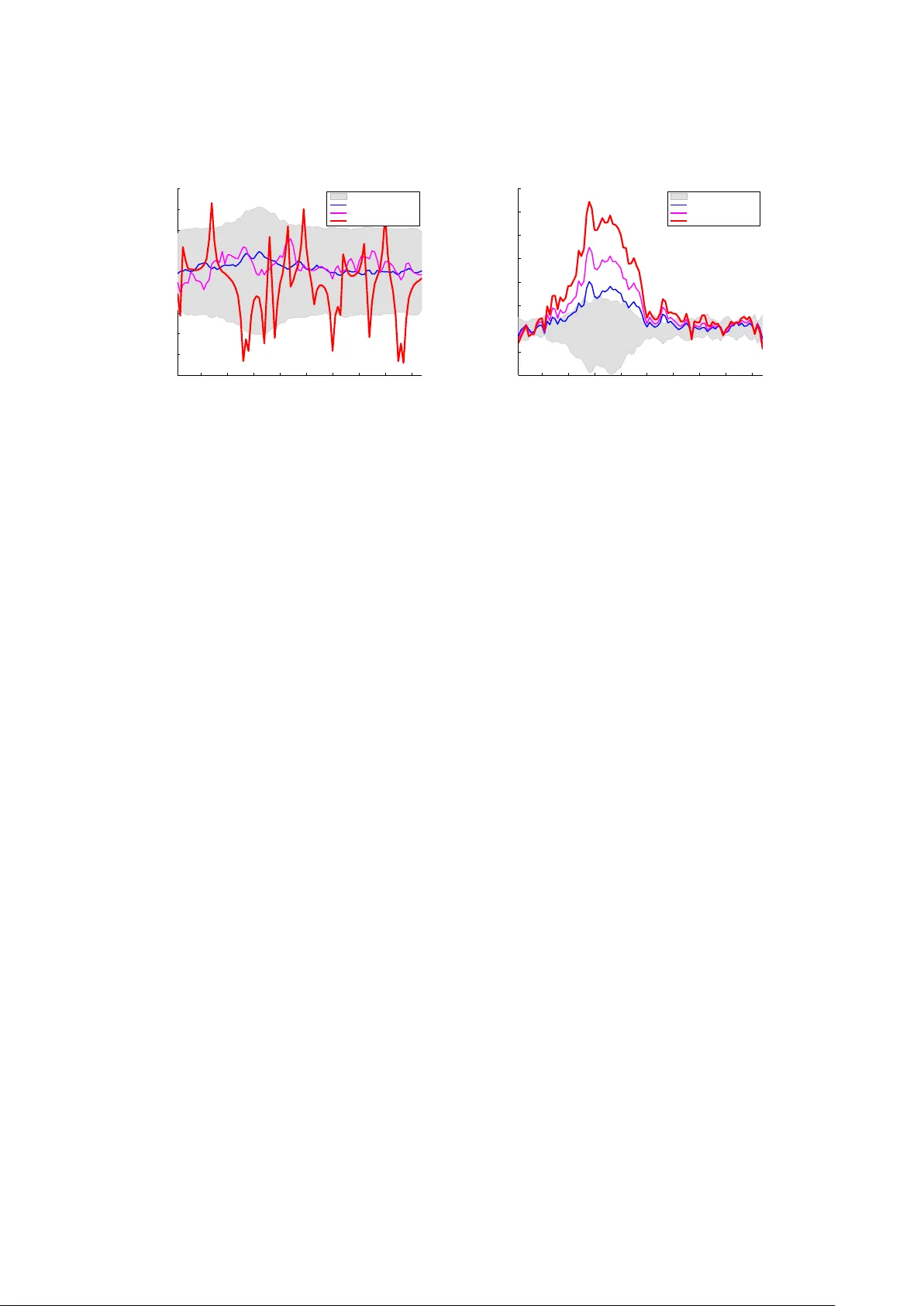
The F eature Imp ortance Ranking Measure ∗ Alexander Zien F raunhofer First/F riedric h Miesc her Lab oratory alexander.zien@first.fraunhofer.de Nicole Kr¨ amer Berlin Institute of T ec hnology nkraemer@cs.tu-berlin.de S¨ oren Sonnen burg F riedric h Miesc her Lab oratory soeren.sonnenburg@tuebingen.mpg.de Gunnar R¨ atsc h F riedric h Miesc her Lab oratory gunnar.raetsch@tuebingen.mpg.de Octob er 22, 2018 Abstract Most accurate predictions are t ypically obtained by learning machines with complex feature spaces (as e.g. induced by kernels). Unfortunately , suc h decision rules are hardly accessible to humans and cannot easily b e used to gain insigh ts ab out the application domain. Therefore, one often resorts to linear models in combination with v ariable se- lection, thereby sacrificing some predictiv e pow er for presumptiv e interpretabilit y . Here, w e introduce the F e atur e Imp ortanc e R anking Me asur e (FIRM), which b y retrosp ectiv e analysis of arbitrary learning mac hines allo ws to ac hiev e b oth excellent predictiv e perfor- mance and sup erior in terpretation. In contrast to standard raw feature w eigh ting, FIRM tak es the underlying correlation structure of the features in to account. Thereb y , it is able to disco v er the most relev an t features, ev en if their app earance in the training data is en- tirely preven ted by noise. The desirable prop erties of FIRM are inv estigated analytically and illustrated in simulations. 1 In tro duction A ma jor goal of machine learning — b ey ond pro viding accurate predictions — is to gain understanding of the inv estigated problem. In particular, for researchers in application areas, it is frequently of high interest to un v eil whic h features are indicative of certain predictions. Existing approac hes to the iden tification of imp ortant features can be categorized according to the restrictions that they impose on the learning mac hines. The most con v enien t access to features is granted by linear learning machines. In this w ork w e consider metho ds that express their predictions via a real-v alued output function s : X → R , where X is the space of inputs. This includes standard mo dels for classification, regression, and ranking. Linearity th us amounts to s ( x ) = w > x + b . (1) One p opular approach to finding imp ortan t dimensions of v ectorial inputs ( X = R d ) is fe a- tur e sele ction , b y which the training pro cess is tuned to mak e sparse use of the a v ailable d ∗ T o appear in the Pro ceedings of the Eur op e an Confer enc e on Machine Le arning and Principles and Pr actic e of Know le dge Disc overy in Datab ases (ECML/PKDD) , 2009. 1 candidate features. Examples include ` 1 -regularized metho ds like Lasso [13] or ` 1 -SVMs [1] and heuristics for non-con v ex ` 0 -regularized formulations. They all find feature w eigh tings w that ha v e few non-zero comp onen ts, for example by eliminating redundan t dimensions. Thus, although the resulting predictors are economical in the sense of requiring few measuremen ts, it can not b e concluded that the other dimensions are unimp ortant: a different (possibly even disjoin t) subset of features ma y yield the same predictiv e accuracy . Being selective among correlated features also predisp oses feature selection metho ds to b e unstable. Last but not least, the accuracy of a predictor is often decreased by enforcing sparsity (see e.g. [10]). In m ultiple kernel learning (MKL; e.g. [5, 10]) a sparse linear com bination of a small set of k ernels [8] is optimized concomitantly to training the kernel machine. In essence, this lifts both merits and detriments of the selection of individual features to the coarser lev el of feature spaces (as induced b y the kernels). MKL th us fails to provide a principled solution to ass essing the importance of sets of features, not to speak of individual features. It is now urban kno wledge that ` 1 -regularized MKL can even rarely sustain the accuracy of a plain uniform kernel com bination [2]. Alternativ ely , the sparsit y requirement may b e dropped, and the j -th comp onen t w j of the trained weigh ts w ma y b e taken as the imp ortance of the j -th input dimension. This has b een done, for instance, in cognitive sciences to understand the differences in human p erception of pictures sho wing male and female faces [4]; here the resulting weigh t v ector w is relatively easy to understand for humans since it can b e represented as an image. Again, this approach may b e partially extended to k ernel mac hines [8], which do not access the features explicitly . Instead, they yield a k ernel expansion s ( x ) = n X i =1 α i k ( x i , x ) + b , (2) where ( x i ) i =1 ,...,n are the inputs of the n training examples. Th us, the w eigh ting α ∈ R n corresp onds to the training examples and cannot be used directly for the interpretation of features. It ma y still be viable to compute explicit weigh ts for the features Φ( x ) induced b y the kernel via k ( x , x 0 ) = h Φ( x ) , Φ( x 0 ) i , provided that the kernel is b enign: it must be guaran teed that only a finite and limited num ber of features are used by the trained machine, suc h that the equiv alent linear formulation with w = n X i =1 α i Φ( x i ) can efficiently b e deduced and represen ted. A generalization of the feature weigh ting approac h that w orks with general kernels has b een prop osed by ¨ Ust ¨ un et. al. [14]. The idea is to characterize input v ariables by their correlation with the w eigh t vector α . F or a linear mac hine as giv en b y (1) this directly results in the w eigh t v ector w ; for non-linear functions s , it yields a pro jection of w , the meaning of whic h is less clear. A problem that all ab ov e metho ds share is that the weigh t that a feature is assigned by a learning mac hine is not necessarily an appropriate measure of its imp ortance. F or example, b y m ultiplying any dimension of the inputs by a p ositiv e scalar and dividing the asso ciated w eigh t b y the same scalar, the conjectured imp ortance of the corresp onding feature can b e c hanged arbitrarily , although the predictions are not altered at all, i.e. the trained learning mac hine 2 is unchanged. An even more practically detrimental shortcoming of the feature weigh ting is its failure to take into account correlations b et ween features; this will b e illustrated in a computational exp erimen t b elo w (Section 3). F urther, all metho ds discussed so far are restricted to linear scoring functions or kernel expansions. There also exists a range of customized imp ortance measures that are used for building decision trees and random forests (see e.g. [11, 12] for an ov erview). In this pap er, w e reach for an imp ortance measure that is “univ ersal”: it shall b e applicable to any learning mac hine, so that we can a v oid the clumsiness of assessing the relev ance of features for metho ds that produce sub optimal predictions, and it shall work for any feature. W e further demand that the imp ortance measure be “ob jective”, whic h has several aspects: it ma y not arbitrarily c ho ose from correlated features as feature selection do es, and it ma y not b e prone to misguidance b y feature rescaling as the w eighting-based metho ds are. Finally , the imp ortance measure shall b e “in telligen t” in that it exploits the connections betw een related features (this will b ecome clearer b elow). In the next section, we briefly review the state of the art with resp ect to these goals and in particular outline a recen t prop osal, whic h is, how ever, restricted to sequence data. Section 2 exhibits ho w w e generalize that idea to con tinuous features and exhibits its desirable prop erties. The next t w o sections are devoted to unfolding the math for several scenarios. Finally , we present a few computational results illustrating the prop erties of our approach in the different settings. The relev an t notation is summarized in T able 1. sym b ol definition reference X input space s ( x ) scoring function X → R w w eigh t vector of a linear scoring function s equation (1) f feature function X → R equation (6) q f ( t ) conditional exp ected score R → R definition 1 Q f feature imp ortance ranking measure (firm) ∈ R definition 2 Q v ector ∈ R d of firms for d features subsection 2.4 Σ , Σ j • co v ariance matrix, and its j th column T able 1: Notation 1.1 Related W ork A few existing feature imp ortance measures satisfy one or more of the ab o v e criteria. One p opular “ob jectiv e” approach is to assess the imp ortance of a v ariable b y measuring the decrease of accuracy when retraining the model based on a random p erm utation of a v ariable. Ho w ev er, it has only a narrow application range, as it is computationally exp ensive and confined to input v ariables. Another approach is to measure the imp ortance of a feature in terms of a sensitivity analysis [3] I j = E "  ∂ s ∂ x j  2 V ar [ X j ] # 1 / 2 . (3) 3 This is both “univ ersal” and “ob jectiv e”. Ho wev er, it clearly do es not tak e the indirect effects in to accoun t: for example, the c hange of X j ma y imply a change of some X k (e.g. due to correlation), which ma y also impact s and thereb y augment or diminish the net effect. Here w e follo w the related but more “intelligen t” idea of [17]: to assess the imp ortance of a feature by estimating its total impact on the score of a trained predictor. While [17] prop oses this for binary features that arise in the context of sequence analysis, the purp ose of this paper is to generalize it to real-v alued features and to theoretically inv estigate some prop erties of this approac h. It turns out (pro of in Section 2.2) that under normality assumptions of the input features, FIRM generalizes (3), as the latter is a first order approximation of FIRM, and b ecause FIRM also tak es the correlation structure in to accoun t. In contrast to the ab o v e mentioned approac hes, the prop osed fe atur e imp ortanc e r anking me asur e (FIRM) also tak es the dependency of the input features in to account. Thereby it is ev en p ossible to assess the importance of features that are not observ ed in the training data, or of features that are not directly considered b y the learning mac hine. 1.2 P ositional Oligomer Imp ortance Matrices [17] In [17], a nov el feature imp ortance measure called P ositional Oligomer Imp ortance Matrices (POIMs) is prop osed for substring features in string classification. Giv en an alphab et Σ, for example the DNA n ucleotides Σ = { A , C , G , T } , let x ∈ Σ L b e a sequence of length L . The k ernels considered in [17] induce a feature space that consists of one binary dimension for eac h p ossible substring y (up to a given maximum length) at eac h p ossible p osition i . The corresp onding w eight w y ,i is added to the score if the substring y is incident at p osition i in x . Th us we ha v e the case of a kernel expansion that can b e unfolded into a linear scoring system: s ( x ) = X y ,i w y ,i I { x [ i ] = y } , (4) where I {·} is the indicator function. Now POIMs are defined b y Q 0 ( z , j ) := E [ s ( X ) | X [ j ] = z ] − E [ s ( X )] , (5) where the expectations are taken with resp ect to a D -th order Marko v distribution. In tuitiv ely , Q 0 measures ho w a feature, here the incidence of substring z at p osition j , w ould c hange the score s as compared to the av erage case (the unconditional exp ectation). Although p ositional sub-sequence incidences are binary features (they are either present or not), they p osses a very particular correlation structure, whic h can dramatically aid in the iden tification of relev an t features. 2 The F eature Imp ortance Ranking Measure (FIRM) As explained in the introduction, a trained learner is defined by its output or scoring function s : X → R . The goal is to quan tify how imp ortan t an y given feature f : X → R (6) of the input data is to the score. In the case of vectorial inputs X = R d , examples for features are simple co ordinate pro jections f j ( x ) = x j , pairs f j k ( x ) = x j x k or higher order in teraction features, or step functions f j,τ ( x ) = I { x j > τ } (where I {·} is the indicator function). 4 W e pro ceed in t w o steps. First, we define the expected output of the score function under the condition that the feature f attains a certain v alue. Definition 1 (conditional expected score) . The c onditional exp e cte d sc or e of s for a fe atur e f is the exp e cte d sc or e q f : R → R c onditional to the fe atur e value t of the fe atur e f : q f ( t ) = E [ s ( X ) | f ( X ) = t ] . (7) W e remark that this definition corresp onds — up to normalization — to the marginal v ariable imp ortance studied b y v an der Laan [15]. A flat function q f corresp onds to a feature f that has no or just random effect on the score; a v ariable function q f indicates an important feature f . Consequen tly , the second step of FIRM is to determine the imp ortance of a feature f as the v ariability of the corresp onding exp ected score q f : R → R . Definition 2 (feature imp ortance ranking measure) . The fe atur e imp ortanc e Q f ∈ R of the fe atur e f is the standar d deviation of the function q f : Q f := q V ar [ q f ( f ( X ))] =  Z R  q f ( t ) − ¯ q f  2 P r ( f ( X ) = t ) dt  1 2 , (8) wher e ¯ q f := E [ q f ( f ( X ))] = R R q f ( t ) P r ( f ( X ) = t ) dt is the exp e ctation of q f . In case of (i) kno wn linear dependence of the score on the feature under inv estigation or (ii) an ill-p osed estimation problem (8) — for instance, due to scarce data —, w e suggest to replace the standard deviation b y the more reliably estimated slop e of a linear regression. As w e will sho w later (Section 2.3), for binary features iden tical feature imp ortances are obtained b y b oth wa ys an yw a y . 2.1 Prop erties of FIRM FIRM generalizes POIMs. As w e will show in Section Section 2.3, FIRM indeed con tains POIMs as special case. POIMs, as defined in (5), are only meaningful for binary features. FIRM extends the core idea of POIMs to con tin uous features. FIRM is “univ ersal”. Note that our feature imp ortance ranking measure (FIRM) can b e applied to a v ery broad family of learning machines. F or instance, it works in b oth classification, regre ssion and ranking settings, as long as the task is mo deled via a real-v alued output function o v er the data p oints. F urther, it is not constrained to linear functions, as is the case for l 1 -based feature selection. FIRM can b e used with any feature space, b e it induced b y a k ernel or not. The imp ortance computation is not even confined to features that are used in the output function. F or example, one may train a kernel machine with a p olynomial k ernel of some degree and afterwards determine the imp ortance of p olynomial features of higher degree. W e illustrate the abilit y of FIRM to quantify the importance of unobserv ed features in Section 3.3. 5 FIRM is robust and “ob jectiv e”. In order to b e sensible, an imp ortance measure is required to b e robust with resp ect to perturbations of the problem and in v ariant with re- sp ect to irrelev ant transformations. Man y successful metho ds for classification and regression are translation-in v ariant; FIRM will immediately inherit this property . Below we sho w that FIRM is also in v arian t to rescaling of the features in some analytically tractable cases (in- cluding all binary features), suggesting that FIRM is generally well-behav ed in this resp ect. In Section 2.4.3 w e show that FIRM is ev en robust with resp ect to the choice of the learning metho d. FIRM is sensitiv e to rescaling of the scoring function s . In order to compare differ- en t learning mac hines with resp ect to FIRM, s should b e standardized to unit v ariance; this yields imp ortances ˜ Q f = Q f / V ar [ s ( X )] 1 / 2 that are to scale. Note, how ever, that the relativ e imp ortance, and thus the ranking, of all features for any single predictor remains fixed. Computation of FIRM. It follo ws from the definition of FIRM that we need to assess the distribution of the input features and that w e hav e to compute conditional distributions of nonlinear transformations (in terms of the score function s ). In general, this is infeasible. While in principle one could try to estimate all quan tities empirically , this leads to an esti- mation problem due to the limited amount of data. Ho wev er, in t w o scenarios, this b ecomes feasible. First, one can imp ose additional assumptions. As we sho w b elo w, for normally distributed inputs and linear features, FIRM can b e approximated analytically , and we only need the co v ariance structure of the inputs. F urthermore, for linear scoring functions (1), we can compute FIRM for (a) normally distributed inputs (b) binary data with kno wn cov ari- ance structure and (c) — as shown b efore in [16] — for sequence data with (higher-order) Mark o v distribution. Second, one can approximate the conditional exp ected score q f b y a linear function, and to then estimate the feature imp ortance Q f from its slop e. As we show in Section 2.3, this approximation is exact for binary data. 2.2 Appro ximate FIRM for Normally Distributed F eatures F or general score functions s and arbitrary distributions of the input, the computation of the conditional exp ected score (7) and the FIRM score (8) is in general intractable, and the quan tities can at b est b e estimated from the data. How ever, under the assumption of normally distributed features, we can deriv e an analytical appro ximation of FIRM in terms of first order T aylor appro ximations. More precisely , we use the follo wing approximation. Appro ximation F or a normal ly r andom variable e X ∼ N  e µ, e Σ  and a differ entiable function g : R d → R p , the distribution of g ( X ) is appr oximate d by its first or der T aylor exp ansion: g ( X ) ∼ N  g ( e µ ) , J e Σ J >  with J = ∂ g ∂ x     x = e µ Note that if the function g is line ar, the distribution is exact. In the course of this subsection, w e consider feature functions f j ( x ) = x j (an extension to linear feature functions f ( x ) = x > a is straigh tforw ard.) 6 First, recall that for a normally distributed random v ariable X ∼ N ( 0 , Σ ), the conditional distribution of X | X j = t is again normal, with expectation E [ X | X j = t ] = t Σ j j Σ j • =: e µ j . Here Σ j • is the j th column of Σ . No w, using the ab o v e approximation, the conditional exp ected score is q f ( t ) ≈ s ( e µ j ) = s (( t/ Σ j j ) Σ j • ) T o obtain the FIRM score, w e apply the appro ximation again, this time to the function t 7→ s ((( t/ Σ j j ) Σ j • ). Its first deriv ative at the expected v alue t = 0 equals J = 1 Σ j j Σ > j • ∂ s ∂ x     x = 0 This yields Q j ≈ s 1 Σ j j  Σ > j • ∂ s ∂ x     x = 0  2 (9) Note the corresp ondence to (3) in F riedman’s pap er [3]: If the features are uncorrelated, (9) simplifies to Q j ≈ v u u t Σ j j ∂ s ∂ x j     x j =0 ! 2 (recall that 0 = E [ X j ]). Hence FIRM adds an additional weigh ting that corresp onds to the dep endence of the input features. These w eigh tings are based on the true co v ariance structure of the predictors. In applications, the true cov ariance matrix is in general not kno wn. Ho w ever, it is possible to estimate it reliably ev en from high-dimensional data using mean-squared-error optimal shrink age [7]. Note that the ab o v e approximation can b e used to compute FIRM for the kernel based score functions (2). E.g., for Gaussian kernels k γ ( x , x i ) = exp  − k x − x i k 2 γ 2  w e hav e ∂ k γ ( x , x i ) ∂ x     x =0 = 2 k ( 0 , x i ) γ 2 x > i = 2 e − ( k x i k 2 /γ 2 ) γ 2 x > i and hence obtain ∂ s ∂ x     x = 0 = N X i =1 α i y i 2 e − ( k x i k 2 /γ 2 ) γ 2 x > i . 7 2.3 Exact FIRM for Binary Data Binary features are b oth analytically simple and, due to their interpretabilit y and versatilit y , practically highly relev an t. Many discrete features can be adequately represented b y binary features, ev en if they can assume more than tw o v alues. F or example, a categorical feature can b e cast in to a sparse binary encoding with one indicator bit for each v alue; an ordinal feature can b e enco ded by bits that indicate whether the v alue is strictly less than each of its p ossibilities. Therefore w e now try to understand in more depth ho w FIRM acts on binary v ariables. F or a binary feature f : X → { a, b } with feature v alues t ∈ { a, b } , let the distribution b e describ ed b y p a = P r ( f ( X ) = a ) , p b = 1 − p a , and let the conditional exp ectations b e q a = q f ( a ) and q b = q f ( b ). Simple algebra sho ws that in this case V ar [ q ( f ( X ))] = p a p b ( q a − q b ) 2 . Thus we obtain the feature imp ortance Q f = ( q a − q b ) √ p a p b . (10) (By dropping the absolute v alue around q a − q b w e retain the directionality of the feature’s impact on the score.) Note that w e can interpret firm in terms of the slope of a linear function. If we assume that a, b ∈ R , the linear regression fit ( w f , c f ) = arg min w f ,c f Z R (( w f t + c f ) − q f ( t )) 2 d P r ( t ) the slop e is w f = q a − q b a − b . The v ariance of the feature v alue is V ar [ f ( X )] = p a p b ( a − b ) 2 . (10) is reco v ered as the increase of the linear regression function along one standard deviation of feature v alue. As desired, the imp ortance is independent of feature translation and rescaling (pro vided that the score remains unchanged). In the following w e can thus (without loss of generalit y) constrain that t ∈ {− 1 , +1 } . Let us reconsider POIMS Q 0 , which are defined in equation (5). W e note that Q 0 ( b ) := q b − ¯ q = p a ( q b − q a ) = p p a /p b Q ( b ); thus Q ( z , j ) can b e reco vered as Q ( z , j ) = Q 0 ( z , j ) p P r ( X [ j ] 6 = z ) / P r ( X [ j ] = z ) . Th us, while POIMs are not strictly a sp ecial case of FIRM, they differ only in a scaling factor whic h dep ends on the distribution assumption. F or a uniform Marko v mo del (as empirically is sufficient according to [17]), this factor is constant. 2.4 FIRM for Linear Scoring F unctions T o understand the prop erties of the prop osed measure, it is useful to consider it in the case of linear output functions (1). 2.4.1 Indep enden tly Distributed Binary Data First, let us again consider the simplest scenario of uniform binary inputs, X ∼ unif ( {− 1 , +1 } d ); the inputs are th us pairwise independent. First w e ev aluate the imp ortance of the input v ariables as features, i.e. w e consider pro- jections f j ( x ) = x j . In this case, we immediately find for the conditional exp ectation q j ( t ) of 8 the v alue t of the j -th v ariable that q j ( t ) = tw j + b . Plugged into (10) this yields Q j = w j , as exp ected. When the features are indep enden t, their impact on the score is completely quan tified by their asso ciated weigh ts; no side effects hav e to b e taken into account, as no other features are affected. W e can also compute the imp ortances of conjunctions of t wo v ariables, i.e. f j ∧ k ( x ) = I { x j = +1 ∧ x k = +1 } . Here we find that q j ∧ k (1) = w j + w k + b and q j ∧ k (0) = − 1 3 ( w j + w k )+ b , with P r ( f j ∧ k ( X ) = 1) = 1 4 . This results in the feature imp ortance Q j ∧ k = ( w j + w k ) / √ 3. This calculation also applies to negated v ariables and is easily extended to higher order conjunctions. Another in teresting t yp e of feature deriv es from the xor-function. F or features f j ⊗ k ( x ) = I { x j 6 = x k } the conditional exp ectations v anish, q j ⊗ k (1) = q j ⊗ k (0) = 0. Here the FIRM exp oses the inability of the linear mo del to capture suc h a dep endence. 2.4.2 Binary Data With Empirical Distribution Here w e consider the empirical distribution as given by a set { x i | i = 1 , . . . , n } of n data p oin ts x i ∈ {− 1 , +1 } d : P r ( X ) = 1 n P n i =1 I { X = x i } . F or input features f j ( x ) = x j , this leads to q j ( t ) = 1 n j t P i : x ij = t w > x i + b , where n j t := | { i | x ij = t } | counts the examples showing the feature v alue t . With (10) w e get Q j = ( q j (+1) − q j ( − 1)) q P r ( X j = +1) P r ( X j = − 1) = n X i =1 x ij n j, x ij  w > x i  r n j, +1 n j, − 1 n 2 It is conv enient to express the v ector Q ∈ R d of all feature imp ortances in matrix notation. Let X ∈ R n × d b e the data matrix with the data p oin ts x i as rows. Then we can write Q = M > Xw with M ∈ R n × d = 1 n × d D 0 + XD 1 with diagonal matrices D 0 , D 1 ∈ R d × d defined by ( D 1 ) j j = 1 2 √ n j, +1 n j, − 1 , ( D 0 ) j j = n j, +1 − n j, − 1 2 n √ n j, +1 n j, − 1 . (11) With the empirical co v ariance matrix ˆ Σ = 1 n X > X , we can th us express Q as Q = D 0 1 d × n Xw + n D 1 ˆ Σw . Here it b ecomes apparent how the FIRM, as opp osed to the plain w , takes the cor- relation structure of the features in to accoun t. F urther, for a uniformly distributed feature j (i.e. P r ( X j = t ) = 1 2 ), the standard scaling is repro duced, i.e. ( D 1 ) j j = 1 n I , and the other terms v anish, as ( D 0 ) j j = 0. F or X con taining each p ossible feature vector exactly once, corresp onding to the uni- form distribution and th us indep enden t features, M > X is the iden tit y matrix (the co v ariance matrix), recov ering the ab o v e solution of Q = w . 2.4.3 Con tin uous Data With Normal Distribution If we consider normally distributed input features and assume a linear scoring function (1), the approximations ab o v e (Section 2.2) are exact. Hence, the exp ected conditional score of 9 an input v ariable is q j ( t ) = t Σ j j w > Σ j • + b . (12) With the diagonal matrix D of standard deviations of the features, i.e. with entries D j j = p Σ j j , this is summarized in q = b 1 d + t D − 2 Σw . Exploiting that the marginal distribution of X with respect to the j -th v ariable is again a zero-mean normal, X j ∼ N (0 , Σ j j ), this yields Q = D − 1 Σw . F or uncorrelated features, D is the square ro ot of the diagonal co v ariance matrix Σ , so that we get Q = Dw . Thus rescaling of the features is reflected b y a corresp onding rescaling of the imp ortances — unlike the plain w eigh ts, FIRM cannot b e manipulated this w a y . As FIRM w eights the scoring v ector b y the correlation D − 1 Σ b et w een the v ariables, it is in general more stable and more reliable than the information obtained by the scoring v ector alone. As an extreme case, let us consider a tw o-dimensional v ariable ( X 1 , X 2 ) with almost p erfect correlation ρ = cor ( X 1 , X 2 ) ≈ 1. In this situation, L1-type metho ds like lasso tend to select randomly only one of these v ariables, sa y w = ( w 1 , 0), while L2-regularization tends to giv e almost equal weigh ts to b oth v ariables. FIRM comp ensates for the arbitrariness of lasso b y considering the correlation structure of X : in this case q = ( w 1 , ρw 1 ), whic h is similar to what would b e found for an equal w eighting w = 1 2 ( w , w ), namely q = ( w (1 + ρ ) / 2 , w (1 + ρ ) / 2). Linear Regression. Here we assume that the scoring function s is the solution of an unregularized linear regression problem, min w ,b k Xw − y k 2 ; thus w =  X > X  − 1 X > y . Plugging this in to the expression for Q from ab o ve yields Q = D − 1 Σ  n ˆ Σ  − 1 X > y . (13) F or infinite training data, ˆ Σ − → Σ , we th us obtain Q = 1 n D − 1 X > y . Here it b ecomes apparen t how the normalization mak es sense: it renders the imp ortance indep enden t of a rescaling of the features. When a feature is inflated b y a factor, so is its standard deviation D j j , and the effect is cancelled by m ultiplying them. 3 Sim ulation Studies W e now illustrate the usefulness of FIRM in a few preliminary computational exp eriments on artificial data. 3.1 Binary Data W e consider the problem of learning the Bo olean formula x 1 ∨ ( ¬ x 1 ∧ ¬ x 2 ). An SVM with p olynomial kernel of degree 2 is trained on all 8 samples that can b e drawn from the Bo olean truth table for the v ariables ( x 1 , x 2 , x 3 ) ∈ { 0 , 1 } 3 . Afterwards, we compute FIRM b oth based on the trained SVM ( w ) and based on the true lab elings ( y ). The results are display ed in Figure 1. 10 1 x1 x2 x3 −1 −0.5 0 0.5 1 0 1 x1 x2 x3 −1 −0.5 0 0.5 1 0 1 x1 x2 x3 −1 −0.5 0 0.5 1 11 x1,x2 x1,x3 x2,x3 −1 −0.5 0 0.5 1 00 01 10 11 x1,x2 x1,x3 x2,x3 −1 −0.5 0 0.5 1 00 01 10 11 x1,x2 x1,x3 x2,x3 −1 −0.5 0 0.5 1 Figure 1: FIRMs and SVM- w for the Bo olean form ula x 1 ∨ ( ¬ x 1 ∧ ¬ x 2 ). The figures displa y heat maps of the scores, blue denotes negative lab el, red p ositiv e lab el, white is neutral. The upp er ro w of heat maps sho ws the scores assigned to a single v ariable, the lo w er ro w shows the scores assigned to pairs of v ariables. The first column sho ws the SVM- w assigning a weigh t to the monomials x 1 , x 2 , x 3 and x 1 x 2 , x 1 x 3 , x 2 x 3 resp ectiv ely . The second column shows FIRMs obtained from the trained SVM classifier. The third column shows FIRMs obtained from the true lab eling. Note that the raw SVM w can assign non-zero w eights only to feature space dimensions (here, input v ariables and their pairwise conjunctions, corresp onding to the quadratic k ernel); all other features, here for example pairwise disjunctions, are implicitly assigned zero. The SVM assigns the biggest weigh t to x 2 , follow ed by x 1 ∧ x 2 . In con trast, for the SVM-based FIRM the most imp ortan t features are x 1 ∧ ¬ x 2 follo w ed by ¬ x 1 / 2 , whic h more closely re- sem bles the truth. Note that, due to the lo w degree of the p olynomial k ernel, the SVM not capable of learning the function “b y heart”; in other words, w e ha v e an underfitting situation. In fact, w e ha ve s ( x ) = 1 . ¯ 6 for ( x 1 , x 2 ) = (0 , 1). The difference in y − FIRM and SVM-FIRM underlines that — as in tended — FIRM helps to understand the learner, rather than the problem. Nevertheless a quite goo d approximation to the truth is found as display ed by FIRM on the true lab els, for which all sev en 2-tuples that lead to true output are found (black blo c ks) and only ¬ x 1 ∧ x 2 leads to a false v alue (stronger score). V alues where ¬ x 1 and x 2 are com bined with x 3 lead to a slightly negative v alue. 3.2 Gaussian Data Here, we analyze a to y example to illustrate FIRM for real v alued data. W e consider the case of binary classification in three real-v alued dimensions. The first tw o dimensions carry the discriminative information (cf. Figure 2a), while the third only contains random noise. 11 The second dimension con tains most discriminative information and we can use FIRM to reco v er this fact. T o do so, we train a linear SVM classifier to obtain a classification function s ( x ). No w we use the linear regression approach to model the conditional exp ected scores q i (see Figure 2b-d for the three dimensions). W e observ e that dimension t w o indeed shows the strongest slop e indicating the strongest discriminative p o w er, while the third (noise) dimension is iden tified as uninformative. −2 0 2 4 −2 0 2 −2 0 2 4 −10 −5 0 5 −2 0 2 −10 −5 0 5 −2 0 2 4 −10 −5 0 5 Figure 2: Binary classification p erformed on contin uous data that consists of t w o 3d Gaussians constituting the tw o classes (with x 3 b eing pure noise). F rom left to right a) Of the raw data set x 1 , x 2 are displa y ed. b) Score of the linear discrimination function s ( x i ) (blue) and conditional exp ected score q 1 (( x i ) 1 ) (red) for the first dimension of x . c) s ( x i ) and q 2 (( x i ) 2 ) for v arying x 2 . As the v ariance of q is highest here, this is the discriminating dimension (closely resembling the truth). d) s ( x i ) and q 3 (( x i ) 3 ) for v arying x 3 . Note that x 3 is the noise dimension and does not contain discriminating information (as can b e seen from the small slop e of q 3 ) 3.3 Sequence Data As shown ab o v e (Section 1.2), for sequence data FIRM is essen tially iden tical to the previously published tec hnique POIMs [17]. T o illustrate its p o wer for sequence classification, we use a to y data set from [9]: random DNA sequences are generated, and for the p ositiv e class the sub-sequence GATTACA is plan ted at a random position centered around 35 (rounded normal distribution with SD=7). As biological motifs are typically not p erfectly conserved, the plan ted consensus sequences are also mutated: for eac h plan ted motif, a single p osition is randomly chosen, and the incident letter replaced b y a random letter (allowing for no change for ∼ 25% of cases). An SVM with WDS kernel [6] is trained on 2500 p ositiv e and as many negativ e examples. Tw o analyses of feature imp ortance are presented in Figure 3: one based on the feature w eigh ts w (left), the other on the feature importance Q (righ t). It is apparent that FIRM iden tifies the GATTACA feature as b eing most imp ortan t at p ositions b et ween 20 and 50, and it ev en attests significant imp ortance to the strings with edit distance 1. The feature w eigh ting w , on the other hand, fails completely: sequences with one or tw o m utations receiv e random imp ortance, and even the imp ortance of the consensus GATTACA itself sho ws erratic b eha vior. The reason is that the app earance of the exact consensus sequence is not a reliable feature, as is mostly occurs m utated. More useful features are substrings of the consensus, as they are less lik ely to b e hit b y a mutation. Consequently there is a large num b er of suc h features that are giv en high w eigh t b e the SVM. By taking into account the correlation of such short substrings with longer ones, in particular with GATTACA , FIRM can reco v er the “ideal” 12 10 20 30 40 50 60 70 80 90 −0.1 −0.08 −0.06 −0.04 −0.02 0 0.02 0.04 0.06 0.08 W (SVM feature weight) sequence position W (SVM feature weight) 7 mutations, ± 1SD 2 mutations, mean 1 mutation, mean 0 mutations (GATTACA) 10 20 30 40 50 60 70 80 90 −40 −20 0 20 40 60 80 100 120 Q (feature importance) sequence position Q (feature importance) 7 mutations, ± 1SD 2 mutations, mean 1 mutation, mean 0 mutations (GATTACA) Figure 3: F eature imp ortance analyses based on (left) the SVM feature weigh ting w and (righ t) FIRM. The shaded area sho ws the ± 1 SD range of the importance of completely irrelev an t features (length 7 sequences that disagree to GATTACA at every p osition). The red lines indicate the p ositional imp ortances of the exact motif GATTACA ; the magen ta and blue lines represent a verage imp ortances of all length 7 sequences with edit distances 1 and 2, resp ectiv ely , to GATTACA . While the feature w eighting approach cannot distinguish the decisiv e motiv from random sequences, FIRM identifies it confiden tly . feature which yields the highest SVM score. Note that this “intelligen t” b eha vior arises automatically; no more domain knowledge than the Marko v distribution (and it is only 0-th order uniform!) is required. The practical v alue of POIMs for real world biological problems has b een demonstrated in [17]. 4 Summary and Conclusions W e prop ose a new measure that quan tifies the relev ance of features. W e take up the idea underlying a recen t sequence analysis method (called POIMs, [17]) — to assess the imp ortance of substrings b y their impact on the exp ected score — and generalize it to arbitrary con tinuous features. The resulting fe atur e imp ortanc e r anking me asur e FIRM has inv ariance prop erties that are highly desirable for a feature ranking measure. First, it is “ob jectiv e”: it is in v arian t with resp ect to translation, and reasonably inv arian t with resp ect to rescaling of the features. Second, to our knowledge FIRM is the first feature ranking measure that is totally “universal”, i.e. which allo ws for ev aluating any feature, irresp ectiv e of the features used in the primary learning machine. It also imposes no restrictions on the learning metho d. Most imp ortantly , FIRM is “intelligen t”: it can identify features that are not explicitly represented in the learning mac hine, due to the correlation structure of the feature space. This allows, for instance, to identify sequence motifs that are longer than the considered substrings, or that are not ev en presen t in a single training example. By definition, FIRM dep ends on the distribution of the input features, which is in general not av ailable. W e show ed that under v arious scenarios (e.g. binary features, normally dis- tributed features), we can obtain appro ximations of FIRM that can b e efficien tly computed from data. In real-world scenarios, the underlying assumptions might not alwa ys be fulfilled. Nev ertheless, e.g. with resp ect to the normal distribution, we can still in terpret the deriv ed form ulas as an estimation based on first and second order statistics only . 13 While the quality of the computed importances does depend on the accuracy of the trained learning machine, FIRM can b e used with any learning framework. It can even b e used without a prior learning step, on the ra w training data. Usually , feeding training lab els as scores into FIRM will yield sim ilar results as using a learned function; this is natural, as b oth are supp osed to be highly correlated. Ho w ev er, the prop osed indirect procedure ma y impro v e the results due to three effects: first, it ma y smooth aw ay lab el errors; second, it extends the set of lab eled data from the sample to the en tire space; and third, it allo ws to explicitly control and utilize distributional information, whic h ma y not b e as pronounced in the training sample. A deeper understanding of such effects, and p ossibly their exploitation in other contexts, seems to b e a rewarding field of future researc h. Based on the unique combination of desirable prop erties of FIRM, and the empirical success of its sp ecial case for sequences, POIMs [17], w e anticipate FIRM to b e a v aluable to ol for gaining insigh ts where alternative tec hniques struggle. Ac kno wledgemen ts This w ork was supp orted in part by the FP7-ICT Programme of the Europ ean Communit y under the P ASCAL2 Net w ork of Excellence (ICT-216886), b y the Learning and Inference Platform of the Max Planck and F raunhofer So cieties, and by the BMBF gran t FKZ 01- IS07007A (ReMind). W e thank P etra Philips for early phase discussion. References [1] K. Bennett and O. Mangasarian. Robust linear programming discrimination of tw o linearly inseparable sets. Optimization Metho ds and Softwar e , 1:23–34, 1992. [2] C. Cortes, A. Gretton, G. Lanc kriet, M. Mohri, and A. Rostamizedeh. Outcome of the NIPS*08 workshop on kernel learning: Automatic selection of optimal k ernels, 2008. [3] J. F riedman. Greedy function approximation: a gradien t b o osting machine. Annals of Statistics , 29:1189–1232, 2001. [4] A. Graf, F. Wichmann, H. H. B¨ ulthoff, and B. Sch¨ olkopf. Classification of faces in man and machine. Neur al Computation , 18:143–165, 2006. [5] G. R. G. Lanckriet, N. Cristianini, L. E. Ghaoui, P . Bartlett, and M. I. Jordan. Learning the kernel matrix with semidefinite programming. Journal of Machine L e arning R ese ar ch , 5:27–72, 2004. [6] G. R¨ atsc h, S. Sonnenburg, and B. Sc h¨ olkopf. RASE: Recognition of alternatively spliced exons in C. ele gans . Bioinformatics , 21(Suppl. 1):i369–i377, June 2005. [7] J. Sc h¨ afer and K. Strimmer. A Shrink age Approac h to Large-Scale Co v ariance Matrix Es- timation and Implications for F unctional Genomics. Statistic al Applic ations in Genetics and Mole cular Biolo gy , 4(1):32, 2005. [8] B. Sch¨ olkopf and A. J. Smola. L e arning with Kernels . Cambridge, MIT Press, 2002. 14 [9] S. Sonnenburg, G. R¨ atsc h, and C. Sc h¨ afer. Learning interpretable SVMs for biological sequence classification. In RECOMB 2005, LNBI 3500 , pages 389–407. Springer, 2005. [10] S. Sonnenburg, G. R¨ atsc h, C. Sch¨ afer, and B. Sch¨ olkopf. Large Scale Multiple Kernel Learning. Journal of Machine L e arning R ese ar ch , 7:1531–1565, July 2006. [11] C. Strobl, A. Boulesteix, T. Kneib, T. Augustin, and A. Zeileis. Conditional v ariable imp ortance for random forests. BMC Bioinformatics , 9(1):307, 2008. [12] C. Strobl, A. Boulesteix, A. Zeileis, and T. Hothorn. Bias in random forest v ariable imp ortance measures: Illustrations, sources and a solution. BMC bioinformatics , 8(1):25, 2007. [13] R. Tibshirani. Regression Shrink age and Selection via the Lasso. Journal of the R oyal Statistic al So ciety, Series B , 58(1):267–288, 1996. [14] B. ¨ Ust ¨ un, W. J. Melssen, and L. M. Buydens. Visualisation and in terpretation of supp ort v ector regression models. Analytic a Chimic a A cta , 595(1-2):299–309, 2007. [15] M. v an der Laan. Statistical inference for v ariable imp ortance. The International Journal of Biostatistics , 2(1):1008, 2006. [16] A. Zien, P . Philips, and S. Sonnenburg. Computing Positional Oligomer Imp ortance Matrices (POIMs). Res. Rep ort; Electronic Publ. 2, F raunhofer FIRST, Dec. 2007. [17] A. Zien, S. Sonnenburg, P . Philips, and G. R¨ atsch. POIMS: P ositional Oligomer Im- p ortance Matrices – Understanding Supp ort V ector Mac hine Based Signal Detectors. In Pr o c e e dings of the 16th International Confer enc e on Intel ligent Systems for Mole cular Biolo gy , 2008. 15