Modeling sparse connectivity between underlying brain sources for EEG/MEG

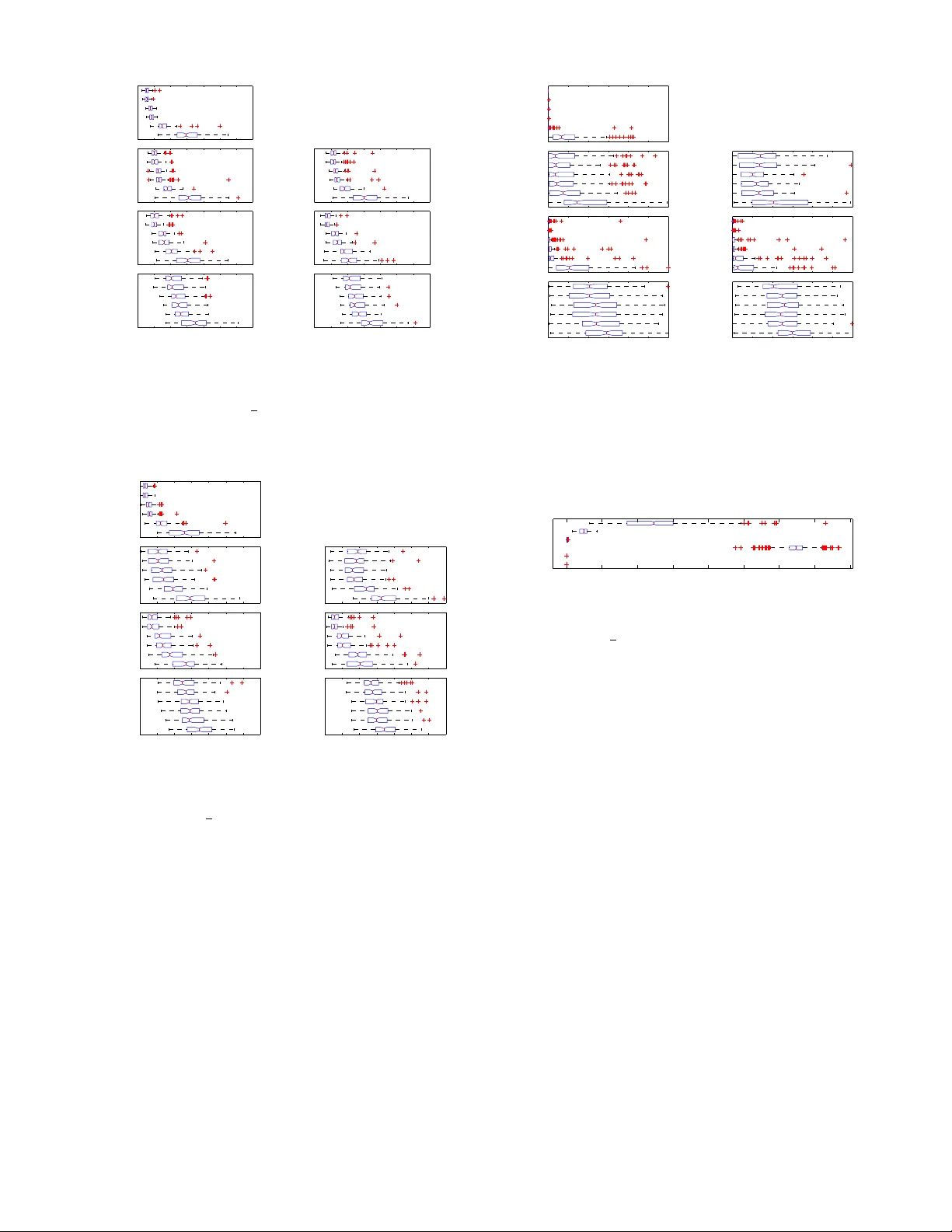
1 Modeling sparse connecti vity between underlying brain sources for EEG/MEG Stefan Haufe, Ryota T omioka, Guido Nolte, Klaus-Robert M ¨ uller and Motoaki Kawanabe Abstract —W e propose a novel technique to assess functional brain connectivity in EEG/MEG signals. Our method, called Sparsely-Connected Sources Analysis (SCSA), can o ver come the problem of volume conduction by modeling neural data innova- tively with the following ingredien ts: (a) the EEG is assumed to be a linear mixture of correlated sources f ollowing a multivariate autoregr essiv e (MV AR) model, (b) the demixing is estimated jointly with the source MV AR parameters, (c) overfitting is av oided by using the Group Lasso penalty . This approach allows to extract the appropriate level cr oss-talk between the extracted sources and in this manner we obtain a sparse data-driven model of functional connectivity . W e demonstrate the usefulness of SCSA with simulated data, and compare to a number of existing algorithms with excellent results. I . I N T RO D U C T I O N A. Functional brain connectivity The analysis of neural connectivity plays a crucial role for understanding the general functioning of the brain. In the past two decades such analysis has become possible thanks to tremendous progress that has been made in the fields of neuroimaging and mathematical modeling. T oday , a multiplicity of imaging modalities exists, allowing to monitor brain dynamics at different spatial and temporal scales. Giv en multiple simultaneously-recorded time-series reflect- ing neural acti vity in dif ferent brain regions, a functional (task- related) connection (sometimes also called information flow or (causal) interaction in this paper) between two regions is com- monly inferred, if a significant time-lagged influence between the corresponding time-series is found. Different measures hav e been proposed for quantifying this influence, most of them being formulated either in terms of the cross-spectrum (e.g., coherence, phase slope index [1]) or an autoregressi ve models (e.g., Granger causality [2], directed transfer function [3], partial directed coherence [4], [5]). B. V olume conduction problem in EEG and MEG In electroencephalography (EEG) and magnetoencephalog- raphy (MEG), sensors are placed outside the head and the problem of volume conduction arises. That is, rather than measuring activity of only one brain site, each sensor captures a linear superposition of signals from all over the brain. This mixing introduces instantaneous correlations in the data, which can cause traditional analyses to detect spurious connectivity [6]. S. Haufe and K.-R. M ¨ uller are with the Berlin Institute of T echnology , Germany . R. T omioka is with the University of T okyo, Japan. G. Nolte and M. Kawanabe are with Fraunhofer Institute FIRST , Berlin, Germany . C. Existing source connectivity analyses Only recently , methods hav e been brought up, which qualify for EEG/MEG connecti vity analysis, since they account for volume conduction effects. These methods can roughly be divided as follows. One type of methods aims at providing meaningful connec- tivity estimates between sensors. The idea here is, that only the real part of the cross-spectrum and related quantities is af fected by instantaneous effects. Thus, by using only the imaginary part, many traditional coupling measures can be made robust against volume-conduction [1], [6]. Another group of methods attempts to inv ert the mixing process in order to apply standard measures to the obtained source estimates. These methods can be further divided into (i) source-localization approaches (where sources are obtained as solutions to the EEG/MEG inv erse problem), (ii) methods using statistical assumptions, and (iii) combined methods. The first approach is pursued, for example, in [7], [8]. Methods in the second category can be appealing, since they avoid finding an explicit in version of the physical forward model. Instead, both the sources and the (de-)mixing transformation are estimated. T o make such decomposition unique, assump- tions have to be formulated, the choice of which is not so straightforward. W e will now briefly revie w some possibilities for such assumptions. Principal component analysis (PCA) and independent com- ponent analysis (ICA) are the most prominent linear decom- position techniques for multiv ariate data. Unfortunately , these methods contradict either with the goal of EEG/MEG connec- tivity analysis (assumption of independent sources in ICA 1 ) or ev en with the physics underlying EEG/MEG generation (as- sumption of orthogonal loadings in PCA). Nevertheless, both concepts hav e been successfully used in more sophisticated ways to find meaningful EEG/MEG decompositions. For example, an interesting use of ICA is proposed in [10]. The authors of this paper do not assume independence of the source traces, but rather argue that this property holds for the residuals of an MV AR model if no instantaneous correlations in the data exist. Hence, in their MV ARICA approach they apply ICA to the residuals of a sensor-space MV AR model. In this work, we first propose a single-step procedure to estimate all parameters (i.e. the mixing matrix and MV AR coefficients) of the linear mixing model of MV AR sources [10] based on temporal-domain conv olutive ICA, instead of the combination of MV AR parameter fitting and demixing by instantaneous ICA. Furthermore, the approach enables us to 1 Although, under some circumstances this approach can be justified [9]. 2 integrate a sparsity assumption on brain connectivity , i.e. on interactions between underlying brain sour ces via the Group Lasso penalty . The additional sparsity prior can av oid over - fitting in practical applications and yields more interpretable estimators of brain connectivity . W e remark that it is hard to incorporate such sparsity priors in MV ARICA, since MV AR is fit to the sensor signals where interactions (i.e. MV AR coefficients) are not at all sparse due to the v olume conduction. The remainder of the paper is organized as follows. In Section II, our procedure will be explained step by step. The correlated source model assumed in this paper will be defined in II-B. The identification procedure called connected sources analysis (CSA) based on the con v oluti ve ICA will be introduced (II-C) and followed by its sparse version, sparse connected sources analysis (SCSA) with the Group Lasso prior (II-D). The relations of our methods with existing approaches such as MV ARICA [10] and CICAAR [11] will be elucidated in detail (II-E). Finally , the optimization algorithms for CSA and SCSA will be explained (II-F). W e implemented two versions for SCSA, one based on L-BFGS and the other by EM algorithm which is slower , but numerically more stable. The next section III will provide our experimental results on simu- lated data sequences emulating realistic EEG recordings. The plausibility of our correlated source model will be discussed with future research directions in the context of computational neuroscience (Section IV), before the concluding remarks (Section V). I I . C O N N E C T E D S O U R C E S A NA LY S I S W I T H S P A R S I T Y P R I O R A. MV AR for modeling causal interactions Autoregressi ve (AR) models are frequently used to define directed “Granger-causal” relations between time-series. The original procedure by Granger inv olves the comparison of two models for predicting a time series z i , containing either past values of z i and z j , or z i only [2]. If inv olvement of z j leads to a lower prediction error , (Granger-causal) information flow from z j to z i is inferred. Since this may lead to spurious detection of causality if both z i and z j are dri ven by a common confounder z ∗ , it is advisable to include the set { z 1 , . . . , z M } \ { z i , z j } of all other observable time series in both models. It has been pointed out, that pairwise analysis can be replaced by fitting one multiv ariate autoregressi ve (MV AR) model to the whole dataset, and that Granger-causal inference can be performed based on the estimated MV AR model coefficients (e.g., [5], [12]). Se veral connectivity measures are deriv ed from the MV AR coefficents [3], [4], but probably the following definition is most straightforward from Granger’ s argument that the cause should always precede the effect. W e say that time series z i has a causal influence on time series z j if the present and past of the combined time series z i and z j can better predict the future of z j than the present and past of z j alone. In the biv ariate case this is equiv alent to saying that for at least one p ∈ { 1 , . . . , P } , the coefficient H ( p ) j i corresponding to the interaction between z j and z i at the p th time-lag is nonzero (significantly different from zero). In the multiv ariate case, Granger causality also includes indirect causes not contained in non-vanishing H ( p ) j i . B. Correlated sources model In this paper we propose a method for demixing the EEG/MEG signal into causally interacting sources. W e start from the same model as in [10]: the sensor measurement is assumed to be generated as a linear instantaneous mixture of sources, which follow an MV AR model x ( t ) = M s ( t ) (1) s ( t ) = P X p =1 H ( p ) s ( t − p ) + ε ( t ) . (2) Here, x ( t ) is the EEG/MEG signal at time t , M is a mixing matrix representing the volume conduction effect, s ( t ) is the demixed (source) signal. The sources at time t are modeled as a linear combination of their P past v alues plus an innov ation term ε ( t ) , according to an MV AR model with coef ficient matrices H ( p ) . In the standard MV AR analysis, the innov a- tion ε ( t ) is a temporally- and spatially-uncorrelated Gaussian sequence. In contrast, we assume here that it is i.i.d. in time and the components are subject to non-Gaussian distributions in order to apply blind source separation (BSS) techniques based on higher-order statistics [10], [11]. For simplicity , we deal with the case that the numbers of sensors and sources are equal and the mixing matrix M is in vertible. When there exist less sources than sensors, the problem falls into the current setting after being preprocessed by PCA [10]. Under our model assumptions, the innov ation sequence can be obtained by a finite impulse response (FIR) filtering of the observation, i.e. ε ( t ) = M − 1 x ( t ) − P X p =1 H ( p ) M − 1 x ( t − p ) (3) = P X p =0 W ( p ) x ( t − p ) , (4) where the filter coefficients are determined by the mixing matrix M and the MV AR parameters { H ( p ) } as W ( p ) =  M − 1 p = 0 − H ( p ) M − 1 p > 0 . (5) Thanks to the non-Gaussianity assumption on the innov ation ε ( t ) , we can use BSS techniques based on higher-order statistics to identify the in verse filter { W ( p ) } . Since we would like to impose sparse connectivity as a plausible prior information later on, it is preferable to apply temporal-domain con volutiv e ICA algorithms. The obtained FIR coefficients { W ( p ) } directly identify the mixing matrix M and the MV AR model of the same order P . C. Identification by convolutive ICA W e use temporal-domain con voluti ve ICA for inferring volume conduction effects and causal interactions between extracted brain signals. The model parameters can be identified 3 based on the mild assumptions that the innov ations are non- Gaussian and (spatially and temporally) independent. For EEG and MEG data, a super-Gaussian is prefered to a sub-Gaussian distribution, assuming that ongoing activity of brain networks is triggered by spontaneous local bursts. W e here adopt the super-Gaussian sech-distribution that was proposed in [11]. The Likelihood of the data under the model is then p ( { x ( t ) } T t = P +1 |{ W ( p ) } ) = | W (0) | T − P T Y t = P +1 D Y d =1 1 π sech ( ε d ( t )) , (6) where ε ( t ) = M − 1 x ( t ) − P P p =1 H ( p ) M − 1 x ( t − p ) . The cost function to be minimized is the negati ve log-Likelihood L ( { W ( p ) } ) = ( P − T ) log | W (0) | − T X t = P +1 D X d =1 log  1 π sech ( ε d ( t ))  . (7) The solution of Eq. ((7)) leads to the estimators of the mixing matrix M and the MV AR coef ficients { H ( p ) } via Eq. ((5)). W e will call this procedure Connected Sources Analysis (CSA). W e remark that the temporal-domain algorithm of con volu- tiv e ICA has obvious indeterminacy due to permutations and sign flips. Howe ver , once we fix a rule to chose one from all candidates, the cost function can be considered as con ve x. D. Sparse connectivity as re gularization In practice, we usually have to consider a long-range lag P to explain temporal structures of data sequences. Ho we ver , this causes too many parameters to be estimated reliably . Maximum-Likelihood estimation may easily lead to overfit- ting, especially if T is small. For this reason, it is advisable to adopt a regularization scheme. Sev eral authors hav e suggested that the complexity of MV AR models can be reduced by shrinking MV AR coefficients tow ards zero. In [12] and [13], MV AR-based functional brain connectivity is estimated from functional magnetic resonance imaging (fMRI) recordings us- ing an ` 1 -norm based (Lasso) penalty , which has the property of shrinking some coefficients exactly to zero. In [5] it is pointed out, that, by using a so-called Group Lasso penalty , whole connections between time-series can be pruned at once. In this approach, all coefficients H ( p ) ij , p = 1 , . . . , P modeling the information flow from s i to s j are grouped together and can only be pruned jointly . From the practical standpoint such sparsification is very appealing, since fewer connections are much easier to interpret. But assuming sparse connectivity in fMRI data might also be justified from a neurophysiological point of view , since under appropriate experimental conditions only a few macroscopic brain areas are expected to show significant interaction. This reasoning also applies to EEG and MEG data. W e note that, besides the penalty-based approach, other strategies for obtaining sparse connectivity graphs exist. For example, post-hoc sparsification can be achie ved for dense estimators by means of statistical testing [5], [14]. Howe ver , due to the compelling built-in regularization, we here adopt Group Lasso sparsification. Before applying our regularization to the cost function of the correlated sources model, it is important to note that the sparsity assumption is only reasonable for the MV AR coefficients { H ( p ) } , but not for the W ( p ) matrices which combine MV AR coefficients and the instantaneous demixing. Hence, in order to apply sparsifying regularization, one has to split the parameters into demixing and MV AR parts again, as in the original model Eq. ((1)). Since the offdiagonal elements { H ( p ) } correspond to interaction between sources, we propose to put a Group Lasso penalty on them analogously to [5]. I.e., we penalize the sum of the ` 2 -norms of each of the groups { H ( p ) d f } , d 6 = f . Let B := M − 1 (= W (0) ) , s ( t ) = B x ( t ) and ˜ s ( t ) = P P p =1 H ( p ) s ( t − p ) . The regularized cost function is L SCSA ( B , { H ( p ) } ) = ( P − T ) log | B | + λ X d 6 = f      H (1) d f , . . . , H ( P ) d f  >     2 − T X t = P +1 D X d =1 log  1 π sech (s d ( t ) − ˜ s d ( t ))  , (8) λ being a positive constant. The solution to Eq. ((8)) for a choice of λ is called the Sparsely-Connected Sources Analysis (SCSA) estimate. E. Relation to other methods The proposed method extends previously suggested MV AR- based sparse causal discov ery approaches [5], [12] by a linear demixing, which is appropriate for EEG/MEG connecti v- ity analysis. Although the correlated sources model Eq. (1) leads to an MV AR model of the observation sequence [10], sparsity of the coefficients cannot be expected after mixing by volume conduction effects. Our method compares with MV ARICA [10], which uses the same model Eq. (1), but estimates its parameters dif ferently . More precisely , the authors of MV ARICA suggest to first fit an MV AR model in sensor- space. The demixing can then be obtained by performing instantaneous ICA on the MV AR innovations, i.e., a dedicated contrast function (Infomax) is used to model independence of the innov ations. The obtained sources follow an MV AR model with time-lagged effects (interactions), but ideally no instantaneous correlations (as caused by volume conduction). It also turns out that the model Eq. (1) is very similar to the conv olutive ICA (cICA) [11], [15]–[17] model. The only difference is that Eq. (1) employs a FIR filter to extract the innov ations, while an infinite response filter (IIR) is usually used in the cICA literature (see, e.g., [11]). This discrepancy is explained by the different philosophies that are associated with both methods. While in our approach the innovations ε ( t ) arise as residuals of a finite-length source-MV AR model, cICA understands them as sources of a finite-length conv olutional mixture. Nev ertheless, our unregularized cost function can be regarded as a maximum-Likelihood approach to an IIR version of conv olutive ICA. This leads us also to a new view of con voluti ve ICA as performing an instantaneous demixing into correlated sources. Hence, it is possible to conduct source connectivity analysis using cICA (see Fig. 1 for illustration). 4 Compared to MV ARICA and time-domain implementations of con volutiv e ICA such as CICAAR [11], our formulation has the advantage that sparse connectivity can easily be modeled by an additional penalty . This is not possible for CICAAR, because CICAAR only indirectly estimates the MV AR co- efficients through their in verse filters. Ho wever , these are generally nonsparse, e ven if the true connecti vity structure is sparse. In verting the in verse coefficients is also generally not possible (recall, that con voluti ve ICA is equi v alent to an infinite-length source-MV AR model). It is furthermore not possible to introduce a sparse regularization for MV ARICA, since this method carries out the MV AR-estimation step in sensor-space, where no sparsity can be assumed. By variation of the regularization parameter, our method is able to interpolate between a fully-correlated source model (comparable to conv olutive ICA) and a model which allows no cross-talk between sources. Interestingly , the latter extreme can be seen as a variant of traditional instantaneous ICA, in which independence is measured in terms of mutual predictability with a Granger-type criterion. ( ) p { } H ( ) p { } W ε x s M (IIR) (FIR) ( ) p M − 1 { } H M M − 1 ε (IIR) M ε (FIR) (ARfit) (ICA) x (a) (b) ( ) p W { } ( ) p A { } ε (FIR) (IIR) x (c) Fig. 1. Relations between (a) SCSA, (b) MV ARICA and (c) CICAAR. All approaches assume a non-Gaussian innovation sequence ε . SCSA and MV ARICA fit an IIR model to the observed sequence x , while CICAAR assumes an FIR filter for it. Therefore, in SCSA and MV ARICA the inv erse filter from x to the innovation ε is an FIR. MV ARICA is a two step approach with AR fitting to the observed sequence x and spartial demixing of the innov ation M ε obtained in the first step. On the other hand, SCSA is a one- step approach which compute the inv erse FIR filter by conv olutiv e ICA. W e remark that the AR fitting in MV ARICA relies only on the second order statistics, which may cause the performance drops compared to CSA. F . Optimization 1) CSA: The gradient of the unregularized cost function Eq. (7) is obtained as ∂ L ∂ W ( p ) d = δ ( p )  ( P − T ) W ( p ) −> e d  + T X t = P +1 tanh P X p =0 W ( p ) d > x ( t − p ) ! x ( t − p ) , (9) where W ( p ) d := W ( p ) > e d , i.e. the d -th column vector of W ( p ) > . W e plug the gradient into a limited memory Broyden- Fletcher-Goldfarb-Shanno (L-BFGS) optimizer [18] 2 and ob- serve that the algorithm always con ver ges to the global op- timum, while only the signs and order of the components may depend on the initialization. W e use W (0) = I and W ( p ) = 0 , p = 1 , . . . , P as a default initializer . 2) SCSA via a modified L-BFGS algorithm: Using sparse regularization, two additional dif ficulties emerge compared to the unregularized cost function. First, using the factor- ization Eq. (5) the guaranteed con ver gence to the minimum observed for CSA is unlikely to be retained. Furthermore, the function Eq. (8) is not dif ferentiable, when one of the terms k ( H (1) d f , . . . , H ( P ) d f ) > k 2 , d 6 = f becomes zero, which is expected to be the case at the optimum. For tackling these difficulties we here propose to use a modified version of the L-BFGS algorithm, which allows joint nonlinear optimization of B and { H ( p ) } , while taking special care of the nondifferentiability of the regularizer . The gradient of Eq. (8) is obtained as ∂ L SCSA ∂ H ( p ) d f = − T X t = P +1 tanh (s d ( t ) − ˜ s d ( t )) s f ( t − p ) + λ H ( p ) d f      H (1) d f , . . . , H ( P ) d f  >     2 (10) and ∂ L SCSA ∂ B d = ( P − T ) B −> e d + T X t = P +1 D X d =1      tanh (s d ( t ) − ˜ s d ( t )) × x ( t ) − P X p =1 x d ( t − p ) H ( p ) d !) . (11) Our modified L-BFGS algorithm checks before each gradient ev aluation, whether some terms k ( H (1) d f , . . . , H ( P ) d f ) > k 2 , d 6 = f are already (close to) zero. If any of the terms equals zero, the gradient is not defined uniquely but as a set (subdifferential). Ne vertheless it is straightforward to compute the element of the subdifferential with minimum norm, whose sign inv ersion is always a descent direction. Care must be taken because in practice we would not find any of the abov e terms exactly equal to zero. Thus we truncate the elements of H corresponding to the terms with small norms below some threshold to zero before computing the minimum norm subgradient. If the minimum is indeed attained at the truncated point, the minimum norm subgradient will be zero. Otherwise the subgradient will driv e the solution out of zero. Further care must be taken in practice to prev ent the solution from oscillating in and out of some zero. 2 W e use an implementation by Naoaki Okazaki, http://www.chokkan.org/software/liblbfgs/ . 5 W e find that, using the outlined optimization procedure, sparse solutions can be found in shorter time, if the solution of the unregularized cost function is used as the initializer . The starting point can be obtained using the inv erse transformation of Eq. (5), which is giv en by B = W (0) (12) H ( p ) = − W ( p ) B − 1 , p > 0 . (13) 3) SCSA via an EM algorithm: Using joint optimization of B and { H ( p ) } , the heuristic pruning of connections might in some cases lead to suboptimal solutions regarding the com- posite cost function. For this reason, we present an alternative optimization scheme, which does not require any heuristic step. The idea here is to alternate between the estimation of both unknowns. Doing so can be justified as an application of the Expectation Maximization (EM) algorithm (see [19]). Estimation of B giv en { H ( p ) } (here called E-step) amounts to solving an unconstrained nonlinear optimization problem. Importantly , this problem is also con vex, in contrast to the joint approach to SCSA parameter fitting. The con ve xity follows from the conca vity of log | X | and log( sech ( ax )) for constant a (and from the f act that the sum of con vex functions is con ve x.). The great advantage of con vex problems is, that they feature a unique (local and global) minimum. In our case, the objectiv e is smooth, so the minimum is guaranteed to be found by the L-BFGS algorithm, making use of the gradient in Eq. (11). Optimization with respect to { H ( p ) } for fixed B (M-step) is more inv olved, since the nondifferentiable Group Lasso regularizer remains. Smooth optimization methods like L- BFGS are unlikely to find the exact solution here. Howe ver , this problem is not as difficult as the joint optimization problem, since it is con ve x. This can be seen from the fact that it is composed of a sum of − log ( sech ( ax )) terms (loss function) and the Group Lasso term (regularizer), which is a sum of ` 2 -norms and thus con ve x. Hence we can solve this problem using the Dual Augmented Lagrangian (D AL) procedure [20], which has recently been introduced as a method for minimizing arbitrary con ve x loss functions with additional Lasso or Group Lasso penalties. Application of D AL requires the loss function and its gradient, the conv ex conjugate (Legendre transform) of the loss function, as well as gradient and Hessian of the conjugate loss. Let s ( t ) = B x ( t ) be the demixed sources and ˜ s ( t ) = P P p =1 H ( p ) s ( t − p ) be their autoregressi ve approximations. The loss function in terms of ˜ s is defined as L M ( ˜ s ) = − T X t = P +1 D X d =1 log  1 π sech ( ˜ s d ( t ) − s d ( t ))  . (14) The gradient is ∂ L M ∂ ˜ s d ( t ) = tanh( ˜ s d ( t ) − s d ( t )) . (15) Let a d ( t ) ( d = 1 , . . . , D , t = P + 1 , . . . , T ) denote the dual variables associated with the Legendre transform. The conjugate loss function is defined on the interval [ − 1 , 1] and ev aluates to D M ( a ) = T X t = P +1 D X d =1 sup ˜ s d ( t )  a d ( t ) ˜ s d ( t ) − log sech ( ˜ s d ( t ) − s d ( t )) π  = T X t = P +1 D X d =1 1 − a d ( t ) 2 log 1 − a d ( t ) 2 + 1 + a d ( t ) 2 log 1 + a d ( t ) 2 − a d ( t )s d ( t ) + log 2 π ! . (16) The gradient of the conjugate loss is giv en by ∂ D M ( a ) ∂ a d ( t ) = 1 2 log 1 + a d ( t ) 1 − a d ( t ) − s d ( t ) . (17) The Hessian is diagonal with elements ∂ 2 D M ( a ) ∂ a d ( t ) 2 = 1 2(1 − a 2 d ( t )) . (18) Having defined the E- and M-steps, we hav e turned a noncon vex estimation problem into a sequence of two conv ex problems, which can both be solved exactly . A final estimate of the model parameters can now be obtained by alternating between E- and M-steps until con ver gence. G. T r eating source autocorr elations Diagonal parts of the MV AR matrices { H ( p ) } model the sources’ autocorrelation and should preferably not be pruned. Howe ver , in some cases numerical stability can be increased if these variables are also penalized, especially if D and P are large. For this reason, we use a slight v ariation of the cost function Eq. (8) in practice, which includes      H (1) 11 , . . . , H ( P ) 11 , . . . , H (1) DD , . . . , H ( P ) DD  >     2 (19) as an additional penalty term. The augmented objective func- tion can be minimized using the techniques presented in Section II-F. I I I . P E R F O R M A N C E U N D E R R E A L I S T I C C O N D I T I O N S W e conducted the following simulations in order to assess the performance of the proposed source connectivity analysis compared to those of existing approaches. A. Data generation W e simulated seven time-series (pseudo-sources) of length N = 2000 according to an MV AR model of order P = 4 . Sev en out of the forty-two possible interactions were modeled by allowing the corresponding offdiagonal MV AR coefficients H ( p ) d f , d 6 = f , 1 ≤ p ≤ P to be nonzero. The innov ations were drawn from the sech-distribution (Note that the assumption of non-Gaussianity is crucial for recov ering mixed sources.). The pseudo-sources were mapped to 118 EEG channels using the theoretical spread of seven randomly placed dipoles. 6 The spread was computed using a realistic forward model [21] which was built based on anatomical MR images of the “Montreal head” [22]. See Fig. 2 for an example illustrating the data generation. In reality , measurements are nev er noise-free and the fol- lowing model holds rather than Eq. (1) x ( t ) = M s ( t ) + ξ ( t ) . (20) Since none of the methods compared here (see below) explicitly models a noise term, it is important to e v aluate their robustness to model violation. T o this end, we constructed additional variants of the pseudo-EEG dataset by adding six different types of noise ξ . The six variants (N1-N6) are summarized in T ABLE I. These variants differ in their degree of spatial and temporal correlation as follows. In variants N1 and N4, ξ i ( t ) , i = 1 , . . . , M were drawn independently for each sensor , i.e., hav e no spatial correlation. For variants N2 and N5 noise terms ξ ∗ i ( t ) , i = 1 , . . . , M were drawn independently for each source . In this case, sources and noise contributions to the EEG share the same cov ariance given by the mixing matrix M , i.e., x ( t ) = M (( s ( t ) + ξ ∗ ( t )) . For the last variants N3 and N6, spatially independent noise sources were simulated at all nodes of a grid cov ering the whole brain, yielding the model x ( t ) = M s ( t ) + M ∗ ξ ∗ ( t ) . Here, in contrast to the previous model, noise contributions are not collinear to the sources. W e further distinguish between noise sources with and without temporal structure. In v ariants (N1- N3), noise terms were drawn i.i.d. from a normal distribution at each time instant t . In v ariants N4-N6, the temporal structure was determined by a univ ariate AR model of order 20, i.e., ξ ∗ ( t ) = P 20 p =1 H ∗ ( p ) ξ ∗ ( t − p ) + ε ∗ ( t ) . Note that, since no time-delayed dependencies between noise sources were modeled, no additional Granger-causal effects were introduced by the noise. W e used a signal-to-noise ratio (SNR) of 2 in all experiments, where SNR is defined as SNR = k M ( s (1) , . . . , s ( T )) k F k ( ξ ∗ (1) , . . . , ξ ∗ ( T )) k F , (21) and k · k F is the Frobenius norm of a matrix. Finally , PCA was applied to the pseudo-EEG to reduce the dimensionality to D = 7 (the original number of sources) by taking just the seven strongest PCA components. One-hundred datasets with different realisations of MV AR coefficients, innov ations and noise were constructed for each category . B. Methods W e tested the ability of ICA, MV ARICA, CICAAR and the two proposed methods CSA and SCSA to reconstruct the sev en sources and their connectivity structure. Although the goal of instantaneous ICA is fundamentally different to source connectivity analysis, it was also included here in the comparison. This is since, ev en if independence of the sources is not fulfilled, ICA might still provide as-least-as-possible dependent components, the connectivity of which might be analyzed. The ICA variant used here is based on temporal decorrelation [23]–[26] (implemented by fast approximate T ABLE I T H E S I X T Y PE S O F N O IS E US E D I N T HE S I MU L A T IO N S . N O I SE W I TH T E MP O R A L C O RR E L A T I O N S T RU CT U R E WAS C RE ATE D U SI N G U N I V A R IAT E A R M O D EL S O F O R DE R 2 0. S P AT IA L C OR R E L A T I ON W A S I NT R OD U C ED U S IN G T HE F OR W A R D M O DE L . W E D IS T I NG U I S H B E TW E E N T H E C A S E , W H ER E N OI S E S O U RC E S C O I N CI D E W I T H T H E T RU E DI P O L ES ( A ) A N D T H E C A SE I N W H I CH N OI S E F R OM A LL B R AI N S IT E S C O N T RI B U TE S TO T HE M E AS U R E ME N T S ( B ) . independent in time correlated in time independent in sensors N1 N4 correlated in sensors a N2 N5 correlated in sensors b N3 N6 joint diagonalization [27]). The number of temporal lags was set to 100. MV ARICA, CICAAR, CSA and SCSA were tested with P ∈ { 1 , 2 , . . . , 7 } temporal lags, where four is the true MV AR model order for CSA, SCSA and MV ARICA. CICAAR has the disadvantage here, that it may generally require extended temporal filters for reconstructing sources following model Eq. (1). Ho we ver , due to computation time constraints, P = 7 was taken as the maximum lag also for this method. For MV ARICA and CICAAR, we used implementations provided by the respectiv e authors. These implementations adopt the Bayesian Information Criterion (BIC) for selecting the appro- priate number of time lags. The same criterion was used to select the model order in CSA and SCSA. The regularization constant λ of SCSA was set by 5 -fold cross-v alidation. SCSA estimates of { H ( p ) } and B were obtained either jointly using the modified L-BFGS algorithm or alternately using 20 additional EM steps. These v ariants are named SCSA and SCS EM here, respectively . C. P erformance measur es The most important performance criterion is the reconstruc- tion of the mixing matrix, since all other rele v ant quantities can basically be derived from it. All considered methods provide an estimate ˆ M − 1 of the demixing, which can be inv erted to yield an estimated mixing matrix. The columns of the mixing matrix correspond to spatial field patterns of the estimated sources, but unfortunately these patterns can generally only be determined up to sign, scale and order . For this reason, optimal pairing of true and estimated patterns as described in [28] was performed. The similarity measure between patterns was slightly modified compared to the one used in [28]. W e used the goodness-of-fit achiev ed by a linear least-squares regression of one to another pattern. For a true pattern M d and an estimated pattern ˆ M f the optimal regression coefficient is c  M d , ˆ M f  = ˆ M > f M d k ˆ M f k 2 (22) and the goodness-of-fit (GOF) is GOF  M d , ˆ M f  = k c ˆ M f − M d k k M d k . (23) 7 Having found the optimal pairing, the colums of M were permuted and scaled to approximate M as good as possible using the optimal regression coefficients. The goodness-of-fit with respect to the whole matrix M was used to ev aluate the quality of the dif ferent decompositions. Additionally , using the optimally-matched mixing patterns, dipole scans were conducted and the deviation of the obtained dipole locations from the true ones was measured. A typical e xample of a mixing pattern estimated by SCSA and the corresponding reconstructed dipole is shown in Fig. 2. Finally , causal discov ery according to [5] was carried out on the demixed sources. The exact technique used was MV AR estimation with Ridge Regression. For the MV AR parameters estimated by Ridge Regression an approximate multiv ariate Gaussian distribution can be deri ved, which was used to test the coefficients for beeing significantly different from zero. An influence from s i to s j was defined, if the p -v alue of one of the coefficients H ( p ) ij , p = 1 , . . . , P fell below the critical value. As a third performance criterion, the area under curve (A UC) score for correctly discovering the interaction structure was calculated by v arying the significance threshold and comparing estimated and true connecti vity matrix for each threshold. Note that this way of connectivity estimation was pursued here in order to treat all methods equally . This was necessary , since not all methods provide built-in connectivity estimates. For SCSA, howe ver , interaction analysis could as well have been done by directly examining MV AR coef ficients. Note further , that using Ridge Regression based testing, the non- Gaussianity of the source MV AR innovations is only indirectly used through the use of the demixing matrix, but not for actual MV AR estimation. For this reason, the MV AR coefficients directly estimated by SCSA may be preferred to a subsequent Ridge Regression step when using SCSA in practice. D. Results Fig. 3 shows, ho w well the mixing matrix was approximated by the different approaches. One boxplot is drawn for the noiseless case (N0) and each of the six noisy variants (N1- N6, see T able I). The plots show the median performance ov er 100 repetitions, as well as the lower and upper quartiles and the extremal values. Outliers (red crosses) were removed. As a result of the simulations, SCSA typically achieves the smallest reconstruction error , followed by CSA, CICAAR, MV ARICA and ICA. In many cases, these dif ferences are also significant, as indicated by notches in the boxes. Correct (de-)mixing matrix estimation affects both the lo- calization error achie v able by applying in verse methods to the estimated patterns and the error of any connectivity analysis performed at the demixed sources. As a result of good mixing matrix approximation, SCSA also achiev es smaller dipole localization errors than all other methods, except in one scenario (sho wn in Fig. 4). The same situation occurs when it comes to estimating the connectivity between sources (Fig. 5). Interestingly , the higher numerical stability we observed for the EM variant of SCSA compared to joint parameter estimation only sometimes leads to superior performance. This may be related to our observation, that the difference between (a) Simulated Dipole (b) Corresponding EEG Pattern (c) Estimated Dipole (d) Estimated EEG Pattern Fig. 2. Example of simulated data (noise type N1) and corresponding reconstruction by SCSA. (a) Simulated dipole. (b) Field pattern describing the dipole’ s influence on the EEG (one column of M ). (d) Field pattern as estimated by SCSA from noisy EEG time series. (c) Reconstructed dipole, obtained from the estimated pattern. the implementations becomes large only for excessi vely large amounts of regularization, which are not optimal in terms of the cross-validation criterion. Another reason might be that the instability of the MV AR coefficients around zero does not play a crucial role in our current ev aluation, since all performance measures used here were solely deriv ed from the demixing matrix. Regarding noise influence it might be said that the relative degradation of performance in the presence of noise is the same for all methods. Generally , noise that is collinear to the sources (N2/N5) seems to be less problematic than noise that is uncorrelated across sensors (N1/N4) and noise with arbitrary spatial correlation structure (N3/N6). Judging from mixing matrix approximation and dipole localization errors, the temporal structure of the noise seems not to affect the performance much. Howe ver , small errors in the (de-)mixing matrix can have quite a negativ e effect on the connectivity estimation, as can be seen in the right part of Fig. 5. The time each method consumed on average for processing one dataset is sho wn in Fig. 6. Most methods finish in rather short time, while the EM implementation of SCSA is in medium range and CICAAR requires the longest time. Howe ver , for SCSA there is still room for improv ement, since the regularization parameter of this method is currently selected by the cross-validation procedure, which could be changed. I V . D I S C U S S I O N Let us recall the assumptions we make to identify individual brain sources and to estimate their interactions. While ICA results in a unique decomposition assuming statistical inde- pendence, such an assumption is inconsistent when studying 8 0 0.1 0.2 0.3 0.4 0.5 0.6 ICA MVARICA CICAAR CSA SCSA SCSA_EM N0 1−GOF Mixing Matrix Approximation Error 0 0.1 0.2 0.3 0.4 0.5 0.6 ICA MVARICA CICAAR CSA SCSA SCSA_EM N1 1−GOF 0 0.1 0.2 0.3 0.4 0.5 0.6 ICA MVARICA CICAAR CSA SCSA SCSA_EM N4 1−GOF 0 0.1 0.2 0.3 0.4 0.5 0.6 ICA MVARICA CICAAR CSA SCSA SCSA_EM N2 1−GOF 0 0.1 0.2 0.3 0.4 0.5 0.6 ICA MVARICA CICAAR CSA SCSA SCSA_EM N5 1−GOF 0 0.1 0.2 0.3 0.4 0.5 0.6 ICA MVARICA CICAAR CSA SCSA SCSA_EM N3 1−GOF 0 0.1 0.2 0.3 0.4 0.5 0.6 ICA MVARICA CICAAR CSA SCSA SCSA_EM N6 1−GOF Fig. 3. Estimation errors of the mixing matrix according to the goodness-of-fit (GOF) criterion. Results are shown for the proposed (Sparsely-) Connected Sources Analysis variants (SCSA EM, SCSA, CSA) and three alternative approaches (CICAAR, MV ARICA, ICA). Different subfigures depict the methods’ performance in the noiseless cass (N0), as well as in the presence of different types of noise (N1-N6, see T ABLE I). 0 1 2 3 4 5 6 7 ICA MVARICA CICAAR CSA SCSA SCSA_EM N0 cm Dipole Localization Error 0 1 2 3 4 5 6 7 ICA MVARICA CICAAR CSA SCSA SCSA_EM N1 cm 0 1 2 3 4 5 6 7 ICA MVARICA CICAAR CSA SCSA SCSA_EM N4 cm 0 1 2 3 4 5 6 7 ICA MVARICA CICAAR CSA SCSA SCSA_EM N2 cm 0 1 2 3 4 5 6 7 ICA MVARICA CICAAR CSA SCSA SCSA_EM N5 cm 0 1 2 3 4 5 6 7 ICA MVARICA CICAAR CSA SCSA SCSA_EM N3 cm 0 1 2 3 4 5 6 7 ICA MVARICA CICAAR CSA SCSA SCSA_EM N6 cm Fig. 4. Localization errors of dipole fits conducted on the estimated mixing field patterns. Results are shown for the proposed (Sparsely-) Connected Sources Analysis (SCSA EM, SCSA, CSA) variants and three alternative approaches (CICAAR, MV ARICA, ICA). Different subfigures depict the methods’ performance in the noiseless cass (N0), as well as in the presence of different types of noise (N1-N6, see T ABLE I). brain interactions. Howe ver , all neural interactions require a minimum delay well within the temporal resolution of electro- physical measurements of brain activity . Hence, it makes sense to assume independent innov ation processes and to model all interactions explicitly using AR matrices. In relation to ICA we pay some price for that: In our case, independence is exploited effecti vely on reduced information contained in the residuals of the model. In principle, this can be a cause for less stable estimates. T o increase stability , we have included sparsity assumptions based on the idea that only a few brain connections can be as strong to be observable in EEG data which is especially the case in the presence of artifacts and background noise. W e emphasize that we assume a linear dynamical model 0 0.1 0.2 0.3 0.4 0.5 0.6 ICA MVARICA CICAAR CSA SCSA SCSA_EM N0 1−AUC Connectivity Error 0 0.1 0.2 0.3 0.4 0.5 0.6 ICA MVARICA CICAAR CSA SCSA SCSA_EM N1 1−AUC 0 0.1 0.2 0.3 0.4 0.5 0.6 ICA MVARICA CICAAR CSA SCSA SCSA_EM N4 1−AUC 0 0.1 0.2 0.3 0.4 0.5 0.6 ICA MVARICA CICAAR CSA SCSA SCSA_EM N2 1−AUC 0 0.1 0.2 0.3 0.4 0.5 0.6 ICA MVARICA CICAAR CSA SCSA SCSA_EM N5 1−AUC 0 0.1 0.2 0.3 0.4 0.5 0.6 ICA MVARICA CICAAR CSA SCSA SCSA_EM N3 1−AUC 0 0.1 0.2 0.3 0.4 0.5 0.6 ICA MVARICA CICAAR CSA SCSA SCSA_EM N6 1−AUC Fig. 5. Estimation errors regarding the source connectivity structure as measured by fitting an MV AR model subsequently to the demixed sources and testing the obtained coefficients for significant interaction. The performance measure reported is the area under the curve (AUC) score obtained by varying the significance level. 0 200 400 600 800 1000 1200 1400 1600 ICA MVARICA CICAAR CSA SCSA SCSA_EM N0−6 sec Runtime Fig. 6. A verage runtime of the proposed (Sparsely-) Connected Sources Analysis variants (SCSA EM, SCSA, CSA) and three alternative approaches (CICAAR, MV ARICA, ICA), taken over all experiments conducted for this study . and non-Gaussian innovation processes, i.e. the only cause of non-Gaussianity is the innov ation process itself. Real brain networks are, of course, more complicated. Howe ver , the question whether nonlinear dynamical models may improve the results or are ev en essential for a correct decomposition is beyond the scope of this paper and will be addressed in the future. Similarly , we assumed the total number of sources to be less or equal the number of channels. Apparently , the significance of this problem decreases when using a large number of channels. V . C O N C L U S I O N Analysing the functional brain connectivity is a hard prob- lem, since volume conduction effects in EEG/MEG measure- ments can gi ve rise to spurious conductivity . In this work we hav e established a nov el connectivity analysis method SCSA that ov ercome these problems in an elegant and numerically appealing manner using Group Lasso. In detail, EEG is mod- eled as a linear mixture of correlated sources, then we estimate jointly the demixing process and the MV AR model (which is the model basis for the correlated sources). For this we assume that the innovations driving the source MV AR process are super-Gaussian distributed and (spatially and temporally) independent. T o avoid overfitting we regularize the model 9 using the Group Lasso penalty . In this manner we can achiev e a data driven interpolation between two extremes: a source model that has full correlations, i.e. con voluti ve ICA and con ventional ICA that does not allow for cross-talk between the extracted sources. In between, our method extracts a sparse connectivity model. W e demonstrate the usefulness of SCSA with simulated data, and compare to a number of existing algorithms with excellent results. Future work will study the link between methods for com- pensating non-stationarity in data such as Stationary Subspace Analysis (SSA, [29]) and our novel connectivity assessment. In addition, we aim to localize the extracted components of connectivity using distributed source models to enhance physiological interpretability (e.g. [30], [31]). A C K N O W L E D G E M E N T This work was partly supported by the Bundesministerium f ¨ ur Bildung und F orschung (BMBF), Fkz 01GQ0850 and by the European ICT Programme Project FP7-224631 and 216886. W e thank Germ ´ an G ´ omez Herrero and Mads Dyrholm for making the source code of their algorithms av ailable, and Nicole Kr ¨ amer for discussions. R E F E R E N C E S [1] G. Nolte, A. Ziehe, V . V . Nikulin, A. Schl ¨ ogl, N. Kr ¨ amer , T . Brismar , and K. R. M ¨ uller , “Robustly estimating the flow direction of information in complex physical systems, ” Phys. Rev . Lett. , vol. 100, p. 234101, Jun 2008. [2] C. Granger , “In vestigating causal relations by econometric models and cross-spectral methods, ” Econometrica , vol. 37, pp. 424–438, 1969. [3] M. J. Kaminski and K. J. Blinowska, “A new method of the description of the information flow in the brain structures, ” Biol Cybern , vol. 65, pp. 203–210, 1991. [4] L. A. Baccal ´ a and K. Sameshima, “Partial directed coherence: a new concept in neural structure determination, ” Biol Cybern , vol. 84, pp. 463–474, Jun 2001. [5] S. Haufe, G. Nolte, K.-R. M ¨ uller , and N. Kr ¨ amer , “Sparse causal discovery in multiv ariate time series, ” in Pr oceedings of the NIPS’08 Causality W orkshop , 2009. [6] G. Nolte, O. Bai, L. Wheaton, Z. Mari, S. V orbach, and M. Hallett, “Identifying true brain interaction from EEG data using the imaginary part of coherency, ” Clin Neurophysiol , vol. 115, pp. 2292–2307, Oct 2004. [7] A. G. Guggisberg, S. M. Honma, A. M. Findlay , S. S. Dalal, H. E. Kirsch, M. S. Berger, and S. S. Nagarajan, “Mapping functional connec- tivity in patients with brain lesions, ” Ann. Neur ol. , vol. 63, pp. 193–203, Feb 2008. [8] L. Astolfi, F . Cincotti, D. Mattia, C. Babiloni, F . Carducci, A. Basilisco, P . M. Rossini, S. Salinari, L. Ding, Y . Ni, B. He, and F . Babiloni, “ Assessing cortical functional connecti vity by linear in verse estimation and directed transfer function: simulations and application to real data, ” Clin Neurophysiol , vol. 116, pp. 920–932, Apr 2005. [9] L. Astolfi, H. Bakardjian, F . Cincotti, D. Mattia, M. G. Marciani, F . De V ico Fallani, A. Colosimo, S. Salinari, F . Miwakeichi, Y . Y am- aguchi, P . Martinez, A. Cichocki, A. T occi, and F . Babiloni, “Estimate of causality between independent cortical spatial patterns during movement volition in spinal cord injured patients, ” Brain T opogr , vol. 19, pp. 107– 123, 2007. [10] G. G ´ omez-Herrero, M. Atienza, K. Egiazarian, and J. L. Cantero, “Measuring directional coupling between EEG sources, ” NeuroIma ge , vol. 43, pp. 497–508, Nov 2008. [11] M. Dyrholm, S. Makeig, and L. K. Hansen, “Model selection for con voluti ve ICA with an application to spatiotemporal analysis of EEG, ” Neural Comput , vol. 19, pp. 934–955, Apr 2007. [12] P . A. V ald ´ es-Sosa, J. M. S ´ anchez-Bornot, A. Lage-Castellanos, M. V e ga-Hern ´ andez, J. Bosch-Bayard, L. Melie-Garc ´ ıa, and E. Canales- Rodr ´ ıguez, “Estimating brain functional connecti vity with sparse multi- variate autoregression, ” Philosophical T ransactions of the Royal Society B , vol. 360, pp. 969–981, 2005. [13] J. M. S ´ anchez-Bornot, E. Mart ´ ınez-Montes, A. Lage-Castellanos, M. V ega-Hern ´ andez, and P . A. V ald ´ es-Sosa, “Uncovering sparse brain effecti ve connectivity: A vox el-based approach using penalized regres- sion, ” Statistica Sinica , vol. 18, no. 4, 2008. [14] D. Marinazzo, M. Pellicoro, and S. Stramaglia, “Kernel method for nonlinear Granger Causality , ” Phys. Re v . Lett. , v ol. 100, p. 144103, 2008. [15] H. Attias and C. E. Schreiner , “Blind source separation and decon- volution: the dynamic component analysis algorithm, ” Neural Comput , vol. 10, pp. 1373–1424, Aug 1998. [16] L. Parra and C. Spence, “Conv olutive blind source separation of non- stationary sources,, ” IEEE T rans. Speech Audio Pr ocessing , vol. 8, no. 3, pp. 320–327, 2000. [17] J. Anem ¨ uller , T . J. Sejnowski, and S. Makeig, “Complex independent component analysis of frequency-domain electroencephalographic data, ” Neural Netw , vol. 16, pp. 1311–1323, Nov 2003. [18] J. Nocedal, “Updating quasi-newton matrices with limited storage, ” Mathematics of Computation , vol. 35, no. 151, pp. 773–782, 1980. [Online]. A vailable: http://www .jstor .org/stable/2006193 [19] R. Neal and G. E. Hinton, “ A view of the em algorithm that justifies incremental, sparse, and other variants, ” in Learning in Graphical Models . Kluwer Academic Publishers, 1998, pp. 355–368. [20] R. T omioka and M. Sugiyama, “Dual augumented lagrangian method for efficient sparse reconstruction, ” IEEE Signal Pr oc Let , vol. 16, no. 2, pp. 1067–1070, 2009. [21] G. Nolte and G. Dassios, “ Analytic expansion of the EEG lead field for realistic volume conductors, ” Phys. Med. Biol. , vol. 50, pp. 3807–3823, 2005. [22] C. J. Holmes, R. Hoge, L. Collins, R. W oods, A. T oga, and A. C. Evans, “Enhancement of MR images using registration for signal averaging, ” J. Comput. Assist. T omogr . , vol. 22, no. 2, pp. 324–333, 1998. [23] L. Molgedey and H. G. Schuster, “Separation of a mixture of indepen- dent signals using time delayed correlations, ” Phys. Rev . Lett. , vol. 72, pp. 3634–3637, Jun 1994. [24] A. Belouchrani, K. Abed-Meraim, J. F . Cardoso, and E. Moulines, “ A blind source separation technique using second-order statistics, ” IEEE T rans Signal Proc , vol. 45, no. 2, pp. 434–444, August 1997. [Online]. A vailable: http://dx.doi.org/10.1109/78.554307 [25] A. Ziehe and K.-R. M ¨ uller , “TDSEP–an efficient algorithm for blind separation using time structure, ” Proc. Int. Conf. on Artificial Neural Networks (ICANN ’98) , pp. 675–680, 1998. [26] A. Ziehe, K.-R. M ¨ uller , G. Nolte, and B.-M. M. a nd G. Curio, “ Artif act reduction in magnetoneurography based on time-delayed second-order correlations, ” vol. 47, no. 1, pp. 75–87, January 2000. [27] A. Ziehe, P . Laskov , G. Nolte, and K.-R. M ¨ uller , “ A fast algorithm for joint diagonalization with non-orthogonal transformations and its application to blind source separation, ” J. Mach. Learn. Res. , vol. 5, pp. 777–800, 2004. [Online]. A vailable: http://portal.acm.org/citation. cfm?id=1016784 [28] P . T ichavsk ´ y and Z. K oldovsk ´ y, “Optimal pairing of signal components separated by blind techniques, ” IEEE Signal Proc Let , vol. 11, no. 2, pp. 119–122, 2004. [29] P . v on B ¨ unau, F . C. Meinecke, F . Kiraly , and K.-R. M ¨ uller , “Estimating the stationary subspace from superimposed signals, ” Physical Review Letters , vol. 103, p. 214101, 2009. [30] S. Haufe, V . Nikulin, A. Ziehe, K.-R. M ¨ uller , and G. Nolte, “Combining sparsity and rotational inv ariance in EEG/MEG source reconstruction, ” Neur oImage , vol. 42, no. 2, pp. 26–738, 2008. [31] S. Haufe, V . V . Nikulin, A. Ziehe, K.-R. M ¨ uller , and G. Nolte, “Esti- mating vector fields using sparse basis field expansions, ” in Advances in Neural Information Processing Systems 21 , 2009.