A Computer Verified Theory of Compact Sets

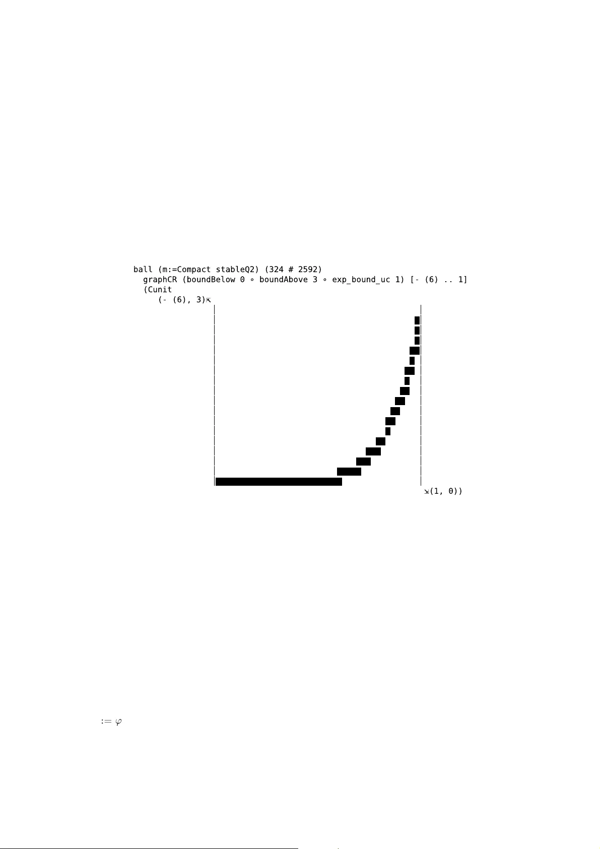
A C o m p u t e r V e ri fi e d T h e or y o f C o m p ac t S e t s ∗ by Russell O’Connor Institute for Computing and Information Science F acult y of Scie nce Radb oud Univer sity Nijmegen Email: r.oconnor@ cs.ru.nl A b s tr a c t C o m p a ct se t s i n c o n st r uc t ive m a th e m a t ic s c a p tu re o u r i n tu i ti o n o f w h a t c o m p u ta b l e s ub - se t s o f th e p l a n e ( or a ny o t h er co m p le t e m e t ri c s p a ce ) o u g ht to b e . A g o o d re p re s e nta t io n o f co m p a c t s e ts p ro vi d e s a n e ffi c ie nt m ea n s o f c r e a ti n g a n d di s pl ay in g im a g es w i th a co m - p u te r . In t h is p ap e r , I b u i ld u p on e x i st in g wo rk a b o u t c om p le t e m e tr ic s pa c e s t o de fi n e c om p a ct s e ts a s t h e c om p le ti o n o f th e s p ac e o f fi n i t e se t s u nd e r t he H au s d o rff m et r ic . Th i s d efi n it i o n al lo w e d m e t o q ui c kl y d eve l o p a c o m p u te r ver ifi e d th eo r y of c om p a ct s et s . I a p p li ed t h i s th e or y to c o m p u te p ro v a bl y co r re c t pl ot s of un if or m l y co nt inu o u s fu n c tio n s . 0 Lice nc e This w ork is hereby relea s ed into the P ublic Domain. T o view a copy o f th e publ ic domain dedi- cation, visit h ttp://creativecommons.org/licenses/pub licdomain/ or send a letter to Cr eativ e Commons, 559 N at han Abb ott W a y, Stanford, California 9 4305, USA . 1 In tr o duct ion How sho uld we define what co mputable s ubsets of the plane ar e ? Sir Roger Penrose ponder s this question at o ne p oint in his b o ok “The Emp eror’s New Mind” [ 9]. Requiring t hat sub sets b e decidable is to o strict; determining if a po in t lies o n the b oundary of a set is undecidable in gen- eral. Penrose gives the unit disc, { ( x , y ) | x 2 + y 2 ≤ 1 } , and t he epigraph of the exp onential func- tion, { ( x , y ) | e xp ( x ) ≤ y } , as examples of sets that intuitively ought to b e considered com- putable [2 ]. Restrictin g one’s a ttent ion to pairs of r a tional or algebraic num ber s may w ork well for t he un it disc, but the b o undary o f the epigraph of the exp onenti al f unction cont ains only one algebraic p oin t. A b etter defi nition i s needed. T o c haracterize computable s ets, w e draw an analogy with re al numbers. The computable real num ber s are rea l num b ers that can b e eff ectiv ely approximated to a rbitrary precis ion. The approximations are usually rational n umbers or dyadic r ational n um b ers. W e can define com- putable sets in a si milar wa y. W e nee d a dense subset of sets that hav e finit ary represen tations. In the ca se o f the plane, the simplest candidate is the finite s ubsets of Q 2 . Again, Q co uld be replac ed wit h the dyadic rationals. H ow do we measure t he accur acy of an approximation? Distances b etween subsets can b e defined b y the Hausdorff metric (se c t ion 3). T o construct the real num b ers, we complete the ration al numbers. By reasoning const ru c- tiv ely (section 2), the real n um b ers generated are alw ays computable. Com pleting the fi nite s ub - sets of Q 2 with the Haus do rff metric yields the co mpact sets (section 5). By reasoning const ruc- tiv ely, t he generat ed compac t sets are alwa ys computabl e! ∗ . T h i s p ap e r i s t o b e p ar t o f th e pr o c e e di n gs of t h e S y mb o li c C o m p u t a ti o n i n S of t wa r e Sc ie n c e A u s tr ia n - J ap a n es e W o r k sh o p ( S C S S 2 0 08 ) .; T h is do c um e nt h a s b e e n w r it te n u s in g t h e G N U T E X M AC S te x t e di to r ( s ee www. texma cs.or g ). 1 The unit disc is constructively compact; it can be effectiv e ly approximated with finit e sets. When a compu ter attempts to d is pla y the unit disc, only a finite set of the pixels can b e shown. So instead of displ a ying a n idea l disc, the computer displays a finite set t ha t appr oximates the disc. This is the key criterio n that P enrose’s examples enjoy. They can b e approximated to arbi- trary pr e c ision and display ed on a raster. T ec hn ically the epigraph of the exp onential function is n ot compact; howev er, it is lo cally compact. One may wish to consider constructiv e lo cally compact sets to b e comput able. Thi s would mean that any fi nite r egion of a c o mputable set has effective app ro ximations of arbitrary precision. This d efinition of co nstructively compact s ets has b een formalized in the Co q pro of assis- tant [11]. Approximations of compact set s can b e rasterized and display ed inside Co q (s e c- tion 6). F or example, fi gure 1 show s a theorem in Co q certifying that a plot is close the exp o - nential function . The plot itself is compu ted fro m the defini tion o f th e graph o f the exp onential function. F ig u r e 1 . A th e o r e m in C o q s ta t in g t h at a pl o t o n a 4 2 by 1 8 r as t er i s c lo s e t o th e g r ap h o f t he e x p o - n ent i al fu n c t i o n on [ − 6 , 1] . The standar d definition of c o mputable sets used in compu table analysis says that a set i s computable if t he dista nce to the se t is a com putable re al-v alued f unction. This definition is equiv alent to our definition u sing computable ap pro ximations (althoug h, t his has not b een veri- fied in Co q). Howev er, I b elieve defining computable sets by eff ectiv e a pp ro ximations of finite sets m ore accu rately matches our in tuition abo ut sets that can b e dr awn by a com puter. 2 Co nstr uc ti v e Math em a tics Usually constructive logic is pr esen ted as a restriction of clas sical logic where pro of b y contradic- tion and the law of the excluded middle are not allow ed . While this is a v ali d point of view, constructive logic can ins tead b e p resen ted as an e xtension o f classical logic. Consider form ulas constructed f rom universal qua n tification ( ∀ ), implica tion ( ⇒ ), conjunc- tion ( ∧ ), true ( ⊤ ), f alse ( ⊥ ), a nd equality for natural numbers ( = N ). Define nega tion b y ¬ ϕ 4 ϕ ⇒ ⊥ . On e can (cons t ructively) p ro v e ¬¬ ϕ ⇒ ϕ ho lds for a n y formula ϕ generated f rom this set of connectives by induction on the structure of ϕ b ecause the atomic for m ulas—which in this cas e are equalities on N —are decidable. Thus, one c a n d educe clas sical resul ts with con- structive pro ofs for formulas generate d from this restr icted set o f conne ctiv es. 2 S ec tion 2 This set of connecti v es is not really restrictive b ecause it can b e u sed t o define the other con- nectives. One can define the classical disjunc tion ( ∨ ˜ ) b y ϕ ∨ ˜ ψ 4 ¬ ( ¬ ϕ ∧ ¬ ψ ) . Simil arly, o ne can define the classical existential quantifier ( ∃ ˜ ) by ∃ ˜ x. ϕ ( x ) 4 ¬∀ x. ¬ ϕ ( x ) . With this full set o f connectives, o ne can pro duce classical mathemat ics. The law of the excluded middle ( ϕ ∨ ˜ ¬ ϕ ) has a constructive pro of when the classical disjunction is us e d. Giv en this presentation of classical log ic, w e can exten d the logic b y adding two new conn ec- tiv es, t he constructive disjunction ( ∨ ) and the cons tructiv e exist e ntial ( ∃ ). T hes e new co nnec- tiv es come equipp ed wit h thei r c onstructive rules of infere nc e (giv en b y natural deduction) [1 2]. These co nstructive conn ectives are slightly stronger than their class ical counterparts. Constru c - tiv e excluded middle ( ϕ ∨ ¬ ϕ ) cannot be deduced in g eneral, and our inductiv e argument that ¬¬ ϕ ⇒ ϕ holds no long er go es through if ϕ uses these c o nstructive connectives. W e wish to us e construct iv e reas oni ng b ecause c on structive pr oo fs ha ve a computation al in terpretatio n. A constructive pro of of ϕ ∨ ψ tells whic h of the tw o disj uncts h old. A pro of of ∃ n : N . ϕ ( n ) giv es a n explicit v alue for n that makes ϕ ( n ) hold. Most impo rtant ly, w e ha ve a functional interpretation of ⇒ and ∀ . A pro of of ∀ n : N . ∃ m : N . ϕ ( n , m ) is interpreted as a func- tion w ith an argument n that returns an m paired wi th a p roo f of ϕ ( n , m ) . The classical f ragment also ad mits this functional in terpretatio n, but formulas in t he classic al fragment typically end in  ⇒ ⊥ . These functions ta ke their arguments and return a pro of of false. O f course, there is no pro of of false , so it must be the case that the arguments cannot simultaneously be sa tisfie d. Therefore, these functions can never be execu ted. In th is sen se, o nly trivial functio ns are created b y pro ofs of cl assical formulas. This i s wh y constructi v e mathe- matics aims t o s trengthen class ic a l results. W e wish to create pro ofs with non-trivial f unctional in terpretatio ns. F rom now on, I will leav e out the word “c onstructive” from phrases like “cons tr uctive disjunc- tion” and “ constructive existential” and simply write “ disjunction” and “ existen tial”. This f ol lows the stand ard pract ice in con structiv e ma thematics of u sing names from classical ma thematics to refer to some stronger co nstructive n otion. I will explicitly use t he word “cla ssical” when I wish to r e fer to cl assical con cepts. 2.1 De p end en tly T yped F un cti ona l Pro gram mi ng This functional in terpretation of constructive deductions is giv en b y the Curry-Howard is omor- phism [12]. This isomorphism asso ciates formulas with dep endent t yp es, and pro ofs o f formulas with fun ctional programs of t he asso ciated dependent types. F or exampl e, the identit y function λx : A. x of type A ⇒ A repres e nts a pro of of the tautology A ⇒ A . T able 1 list s t he asso c iation b etween logical co nn ectives and type constructors . Logical Connec tiv e T yp e Constructor implication: ⇒ function t yp e: ⇒ conjunction: ∧ pro duct t ype: × disjunction: ∨ disjoint union typ e: + true: ⊤ unit typ e: () false: ⊥ vo id t ype: ∅ for all: ∀ x. ϕ ( x ) dep endent function t yp e: Π x. ϕ ( x ) exists: ∃ x . ϕ ( x ) dep endent pair typ e: Σ x. ϕ ( x ) T a b l e 1 . T he a s so c ia ti o n b e t we e n fo r mu la s an d ty p e s gi ve n by th e Cu rr y -H o w ar d is o m o rp h is m In dep endent t yp e theory, functi ons from v alues to types are allowed. Using types parametrized b y v alues, one can create dep endent pair type s, Σ x : A. ϕ ( x ) , and dep endent fun c- tion t yp es, Π x : A. ϕ ( x ) . A de p en den t pair consists o f a va lue x of typ e A and an v alue of type ϕ ( x ) . The type of the s e cond v alue dep e nds on the first v alue, x . A dep endent function is a function from the typ e A to the typ e ϕ ( x ) . The type of the result dep en ds on the v alue of the input. C o nst ructiv e M a them a t ic s 3 The asso ciation b etween logical connectives and types can b e carried ov er to cons tr uctiv e mathematic s. W e as soc iate mathematica l structures, s uc h as the natural n umbers, wit h induc- tiv e types in function al programming languag es. W e a ssocia te a tomic formulas w ith functions returning t yp es. F or example, we can define equality on th e natura l num b ers, x = N y , a s a recur- sive function: 0 = N 0 4 ⊤ S x = N 0 4 ⊥ 0 = N S y 4 ⊥ S x = N S y 4 x = N y One catch is t ha t gener al recursio n is not a llow ed when crea ting funct ions. The problem is that general recursion allows one to create a fixp oint op erator fix : ( ϕ ⇒ ϕ ) ⇒ ϕ tha t corr espo nds to a pro of of a logical inconsistency. T o prev en t th is , we allow o nly well-founded rec ur sion ov er an argument with an induct ive type. Be cause well-founded recursio n e n sures that functions alwa y s terminate, the language is not T uring complete. Howev er, one can still ex press fast growing functions lik e th e Ack ermann functio n without difficulty [12]. Because pro ofs and programs a re wr itten in the same language, we can freely mix th e t w o. F or example, in my previous wo rk [7], I repr e sen t the real num b ers by the t yp e ∃ f : Q + ⇒ Q . ∀ ε 1 ε 2 . | f ( ε 1 ) − f ( ε 2 ) | ≤ ε 1 + ε 2 . (1) V alues of this t yp e ar e pairs of a function f : Q + ⇒ Q an d a proo f of ∀ ε 1 ε 2 . | f ( ε 1 ) − f ( ε 2 ) | ≤ ε 1 + ε 2 . Th e idea is that a real n um b er is represented by a f unction f that maps an y requested precision ε : Q + to a rational approximation of the r eal n um b er. Not ever y funct ion of type Q + ⇒ Q represents a real number. Onl y those funct ions that hav e coherent approxim ations sho uld b e allowed. The pro of ob ject pa ir ed with f witnesses the fact that f ha s coherent app ro ximations. This is one example of how mixing functions and formulas allows one to create precise datatyp es. 2.2 No ta tio n I will use the functional st yle of defining m ultiv ariate functions wi th C urried t ype s . A binary function will hav e t yp e X ⇒ Y ⇒ Z instead of X ∧ Y ⇒ Z ( ⇒ is taken to b e righ t asso ciative). T o ease reada bility, I will still write bina ry f unction application as f ( x , y ) , even t hough it should r eally b e f ( x )( y ) . Anonymous functions are wri tten using la m b da expressions . A f unction o n natural n um b ers that doubles its input is w r itten λx : N . 2 x . The ty p e of the paramet er will b e omitted when it is clear f rom context what it should b e. The t ype of prop ositions is ⋆ . Predica tes a re represented by f unctions t o ⋆ . Th ese pred i- cates are o ften used where p ower sets are used in classica l mathem atics. The type X ⇒ ⋆ can be seen a s the po w er set of X . I will often w rite x ∈ A in place of A ( x ) when A : X ⇒ ⋆ and x : X . The notation x ∈ l is a lso us ed when l is a fin ite enumeration (section 4). Also x ∈ S will b e used w hen S is a compact se t (section 5 ). The t yp es will make it clear what the in ter pretation of ∈ should b e. I will u se shorthand t o combine mem ber ship with qua n tifiers. I wil l write ∀ x ∈ A . ϕ ( x ) fo r ∀ x. x ∈ A ⇒ ϕ ( x ) , and ∃ x ∈ A . ϕ ( x ) will me a n ∃ x. x ∈ A ∧ ϕ ( x ) . Quotient typ es are not used in th is theory. In place of quotients, setoids a re used. A set oid is a dep endent reco rd containing a type X (its car rier), a relation ≍ : X ⇒ X ⇒ ⋆ , and a p roo f that ≍ is an equiv alence relation. When w e de fine a funct ion on setoid, we usually pro v e it i s r esp e ctful , meanin g it re s pect s th e set oid eq uiv alence relatio ns on its doma in a nd codo main. Resp ectful functions w i ll also b e called morphisms . I will often write f ( x ) when f is a reco rd (or existen tial) with a fu nction as its carr ier (or witness) and leav e implicit the pro j e ction of f in to a f unction. 4 S ec tion 2 3 Me t ric Spaces T radition ally, a m etric space is defined as a set X with a met ric function d : X × X ⇒ R 0+ satis- fying c e rt ain axioms. The usual constructive formulation requires d b e a com put able function. In m y previous w ork [7], I ha ve found it u seful to take a more relaxed defi nition for a metric space that do es not require the met ric be a function. Instead, I represent the metric via a resp ectful b all relation B : Q + ⇒ X ⇒ X ⇒ ⋆ sa tisfying fi v e axioms: 1. ∀ x ε. B ε ( x , x ) 2. ∀ x y ε . B ε ( x , y ) ⇒ B ε ( y , x ) 3. ∀ x y z ε 1 ε 2 . B ε 1 ( x , y ) ⇒ B ε 2 ( y , z ) ⇒ B ε 1 + ε 2 ( x , z ) 4. ∀ x y ε . ( ∀ δ . ε < δ ⇒ B δ ( x , y ) ) ⇒ B ε ( x , y ) 5. ∀ x y . ( ∀ ε. B ε ( x , y ) ) ⇒ x ≍ y The ball relati on B ε ( x , y ) expresses that the points x and y are within ε of each oth er. I call this a ball relationship be c a use the partially applied relation B ε ( x ) : X ⇒ ⋆ is a predicate that represents the ball of radius ε ar ound the p oint x . The first two axioms a re reflexivity a nd sym- metry o f the ball rel ationship. T he third axiom is a v ersion of the t riangle inequ alit y. The fourth axiom states that the ba lls are closed balls. Closed balls are u sed b ecau se b eing closed is u sually a classica l formula. This m eans they can be igno red during comp utation b ecause they hav e no com putational conten t [4]. W e wan t to minim ize the amount of compu ta- tion n eeded to get ou r construct iv e results. The fi fth axiom states the identit y of indisc e rnibles. This means t hat if t w o p oints a re arbi- trarily close together then they are equiv alent. Th e rev erse implication follows from the reflex- ivit y axiom a nd the fact that B is resp ectful. In s ome ins t ances, axiom 5 can be consider ed as the definition o f ≍ on X . F or example, Q can b e equipp ed with the usual metric by defi ning the ball rela tio n as B ε Q ( x , y ) 4 | x − y | ≤ ε. This d efinition satisfies all the requ ired axioms. 3.1 U nif orm C on tin uit y W e are interested in the category of metric space s with unif ormly cont inuous funct ions b etween them. A f unction f : X ⇒ Y b etween two metric spaces is uniformly c ontinuous with mo dulus µ f : Q + ⇒ Q + if ∀ x 1 x 2 ε. B µ f ( ε ) X ( x 1 , x 2 ) ⇒ B ε Y ( f ( x 1 ) , f ( x 2 )) . W e ca ll a funct ion uniformly c o ntinuous if it is uniform ly cont inuous with some mo dulus. W e use notation X → Y with a single bar arrow to denote th e t yp e of unifo rmly con tin uous functions from X to Y . This r e cord type consis ts of three parts, a function f of type X ⇒ Y , a mo dulus of contin uity, a nd a p roo f th at f is u niformly contin uous with t he given mod ulus. Again, we wil l leav e the p ro jection t o the function typ e im plicit and allow u s to write f ( x ) when f : X → Y and x : X . 3.2 Cl as sifi cat io n of Metr ic S pa ces There is a hierarch y of classes th at m etrics can b elo ng to. The stron gest class of m etrics are the de cidable metrics where ∀ x y ε. B ε X ( x , y ) ∨ ¬ B ε X ( x , y ) . The const ructiv e disjuncti on h ere implies th ere is an algo rithm for compu ting whether tw o p oints are wit hin ε of each other or no t. The metric on Q has this pro per t y; howev er , the metric on R do es n ot b ecause of the lack of a dec id able e q ualit y. M et r ic S p aces 5 The next strongest cla ss of metrics is what I ca ll lo c ate d me trics . These metrics hav e the prop erty ∀ x y ε δ . ε < δ ⇒ B δ X ( x , y ) ∨ ¬ B ε X ( x , y ) . This is simil ar to b eing decid able, bu t there is a littl e extra wiggle r oo m. If x and y are b etween ε and δ fa r a part, then the algorithm has t he option of either re tu rn a pro o f of B δ X ( x , y ) or ¬ B ε X ( x , y ) . This extra flexibi lit y a llows R to b e a lo cated metric. Every decid able metric is also a lo cated metric. Some metrics are not lo cated. The stan dard sup-metric on functi ons b etween metric spaces may not b e lo cated. The weakes t class of metrics we will discuss are the stable metri cs . A metric is st able when ∀ x y ε. ¬¬ B ε X ( x , y ) ⇒ B ε X ( x , y ) . Every loca ted metric is stable. A lthough we will d iscuss the possibil it y of non-stable metrics in section 7, it app ea rs that m etric spaces used in practice are stable. Th is work relies crucia lly on stability at on e p oint, so we will b e assumin g that met ric space s are s table throug hout this pap er. 3.3 Co m ple te M et rics Giv en a metri c space X , one can cr eate a new metric space called th e c omp letion of X , or simply C ( X ) . The t ype C ( X ) is defi ned to b e ∃ f : Q + ⇒ X . ∀ ε 1 ε 2 . B ε 1 + ε 2 X ( f ( ε 1 ) , f ( ε 2 )) with th e ball relation defi ned to b e B ε C ( X ) ( x , y ) 4 ∀ δ 1 δ 2 . B δ 1 + ε + δ 2 X ( x ( δ 1 ) , y ( δ 2 )) . The definition of C ( X ) ma y lo ok familiar. It is a g eneralization of the typ e that I gav e for real nu mbers in equatio n 1. In fact, in m y actu al implementation the real num b ers are defi ned to be C ( Q ) . A complete metric c omes equipp ed with an injection fro m th e original space unit : X → C ( X ) and a functio n b ind : ( X → C ( Y ) ) ⇒ ( C ( X ) → C ( Y )) tha t lifts u niformly contin uous functions with doma in X to uniformly contin u ous function wi th domain C ( X ) . O ne of the most common wa y o f creating f unctions that op erate on complete metric s paces is by using bind. One first defines a f unction on X , whi c h is easy to work with when X is a discrete space. Then one pro ves the funct ion is uniformly cont inu ous. After that, bind do es the rest of the work. A second, similar wa y of cr e ating funct ions wit h com plete do mains is by usi ng map : ( X → Y ) ⇒ ( C ( X ) → C ( Y )) . The function m ap ca n b e defined by map ( f ) 4 bind ( unit ◦ f ) , but in my implementation, map is mo re fundame n tal than bind [7] . I will use t he following notation: x ˆ 4 unit ( x ) f ˇ 4 bind ( f ) f ¯ 4 map ( f ) The complet ion op eration, C , a nd the functio ns unit and bind together f orm a standard con- struction called a monad [6]. M onads hav e b een used in functional programs to capture many different computatio nal notions including exceptions, m utable state, and input/output [13]. W e will see another example of a monad in section 4. 3.4 Pr oduct M etr ic s Giv en tw o metric spaces X and Y , the ir Cartesian pro duct X × Y f orms a metric space with the standard sup-metric: B ε X × Y (( x 1 , y 1 ) , ( x 2 , y 2 )) 4 B ε X ( x 1 , x 2 ) ∧ B ε Y ( y 1 , y 2 ) 6 S ec tion 3 The pro duct metric interacts nicely with the completion op eration. There i s an isomo rphism b etween C ( X × Y ) and C ( X ) × C ( Y ) . One direct ion I call c ouple . The other direction is defined by lifting th e pro jection functions: couple : C ( X ) × C ( Y ) → C ( X × Y ) π 1 ¯ : C ( X × Y ) → C ( X ) π 2 ¯ : C ( X × Y ) → C ( Y ) W e de n ote coupl e ( x , y ) b y h x , y i . Th e followin g lemmas p ro v e that these fun ctions form an iso - morphism. h π 1 ¯ ( z ) , π 2 ¯ ( z ) i ≍ z ( π 1 ¯ h x , y i , π 2 ¯ h x , y i ) ≍ ( x , y ) 3.5 Ha usdor ff M et ric s Giv en a metric space X , w e can try to put a metric on predicate s (subsets) of X . W e sta rt b y defining the Hausdo rff hem imetric. A hemimetric is a metric without the symme try and ide ntit y of ind iscernibles r equirement. W e define the hemim etric relation ov er X ⇒ ⋆ as H ε X ⇒ ⋆ ( A , B ) 4 ∀ x ∈ A . ∃ ˜ y ∈ B . B ε ( x , y ) . Notice the use of the classical existen tial in this definition . In gener al, w e do not need to know which p oint in B is close to a g iv en p oint in A ; it is sufficient to know one exists without knowing which one. F urthermo re, there are cases when we cannot know which p oint in B is close to a giv en p oint in A . This relation i s reflex iv e and satisfies t he triangle inequality. It is n ot symmetric. W e define a sym metric relatio n by B ε X ⇒ ⋆ ( A , B ) 4 H ε X ⇒ ⋆ ( A , B ) ∧ H ε X ⇒ ⋆ ( B , A ) . This rel ationship i s reflexive, symmetr ic, and sa tisfies the triangle inequality. Notice that if B ⊆ A t hen H ε ( A , B ) holds for a ll ε . The hemimetric captu res the subs et relationsh ip. If B ⊆ A and A ⊆ B (i.e. A ≍ B ), then B ε ( A , B ) holds for all ε . Howev er, axiom 5 for metric spaces requires the rev erse implicati on; if B ε ( A , B ) holds fo r all ε , then w e wan t A ≍ B . Unfortunately, this does not hold in gen eral. Neither do es the closedness prop ert y re quired by axiom 4 hold. T o make a true metric space, we need to fo cus on a sub class of predica tes that hav e m ore structu re. 4 Fin ite En umer ation s A fin ite enumeration of po ints fro m X i s represented by a list. A p oint x is in a finite en umera- tion if th ere classica lly exists a p oint in the list t hat is equiv alent to x . W e are n ot required to know which p oin t in the list is equiv alent to x ; we only need to know th at there is one. An equiv alent definition can be given by w ell-founded recursion on lists: x ∈ n il 4 ⊥ x ∈ cons y l 4 x ≍ y ∨ ˜ x ∈ l T wo finite enu merations are con s idered equiv a len t if they h a v e exactly the same memb ers: l 1 ≍ l 2 4 ∀ x. x ∈ l 1 ⇔ x ∈ l 2 If X is a metric space, th en the spa ce of finite enumerations ov er X , F ( X ) , is a lso a met ric space. The Hausdo rff metric with the members hip predicat e defines the ba ll relation: B ε F ( X ) ( l 1 , l 2 ) 4 B ε X ⇒ ⋆ ( λx. x ∈ l 1 , λy . y ∈ l 2 ) This bal l relation is both closed (axiom 4) and is com patible with o ur equiv al ence relation for finite e n umerations (axiom 5), so t his truly is a metric space. F in ite E n ume ra tio ns 7 Finite en umerat ions also form a mona d (I ha ve y et t o v erify this in Co q). The unit : X → F ( X ) funct ion creates an en umeration with a single member. The bind : ( X → F ( Y ) ) ⇒ ( F ( X ) → F ( Y )) fun ction takes an f : X → F ( Y ) an d applies i t to every ele- ment of an en umeration l : F ( X ) and returns the u nio n of the result s. 4.1 Mi xi ng Cla ss ica l and Con struc t iv e R easo nin g Proving the ball relation for finite enumerations is closed mak es essential use of classical r e a- soning. Given ε , supp ose B δ F ( X ) ( l 1 , l 2 ) holds whenever ε < δ . W e need t o show t hat B ε F ( X ) ( l 1 , l 2 ) holds. By the definition of the metric, this requires pro vi ng (in part) ∀ x ∈ l 1 . ∃ ˜ y ∈ l 2 . B ε X ( x , y ) . F rom our assumptions , we know that ∀ x ∈ l 1 . ∃ ˜ y ∈ l 2 . B δ X ( x , y ) holds for every δ greater than ε . If we had us ed a constructive exis tent ial in the definiti on of the Hausdorff hem imetric, we would hav e a problem. Eac h differen t v alue δ could pro duce a differ ent y witnessin g B δ X ( x , y ) . In ord er to us e the cl osedness prop ert y from X to concl ude B ε X ( x , y ) , we need a single y such that B δ X ( x , y ) holds for all δ g reater than ε . Classically w e wo uld use the infinite pigeon hole prin- ciple to find a single y that oc c ur s in finitely often in the s tream of y s pro duced from δ ∈ { ε + 1 n | n : N + } . Suc h reasoning do es n ot work c o nstructively. Given an infi nit e strea m of ele- ments drawn from a finite enumeration, there is n o algor ithm that will de termine wh ic h o ne o ccurs infin itely oft e n. F ortunate ly, b ecause w e used classical quantifi ers in the definition of the Hausdorff metric, we can app ly the the in finite pigeon hole principle to t his problem. W e classically know t here i s some y that o ccurs infinitel y often when δ ∈ { ε + 1 n | n : N + } , even if w e do not know which one. F or such y , B δ X ( x , y ) holds for δ a rbitrarily clos e to ε , and therefore B δ X ( x , y ) must hold for a ll δ greater than ε . B y the closedness prop ert y fo r X , B ε X ( x , y ) holds as required. Th e other half of the definition o f B ε F ( X ) ( l 1 , l 2 ) is handled similarly. Recall that the classical f rag men t of constructive logic requires that pro of by contradiction hold for a tomic f orm ulas in order to deduce the r ule ¬¬ ϕ ⇒ ϕ . Because B ε X ( x , y ) is a param- eter, w e do not know if it is co nstructed o ut of cla ssical connecti v es. T o us e the classica l rea- soning needed to apply the pigeon hole principle, we assume that ¬¬ B ε X ( x , y ) ⇒ B ε X ( x , y ) holds. This i s the crucial p oint where stability of the metric for X is used. 5 Co mpact Set s Completing the metric space of fi nite enumerations yi elds a metric space of compact se ts: K ( X ) 4 C ( F ( X )) The idea is that ev ery co mpa ct set can b e represented as a limi t of fin ite enumerations that approximate it. In ord e r for a com pact set to b e c onsidered a set, w e need to define a member - ship rel ation. The memb ership is no t ov er X b ecause compac t sets are supp osed to be complete and X may not b e a complete space itself. Instead, memb ership is ov er C ( X ) , and it is defined for x : C ( X ) and S : K ( X ) as x ∈ S 4 ∀ ε 1 ε 2 . ∃ ˜ y ∈ S ( ε 2 ) . B ε 1 + ε 2 X ( x ( ε 1 ) , y ) . A p oint is consider ed to be a mem b er of a compact set S if it is arbitrarily close to bein g a member of all app ro ximations of S . Thus K ( X ) r epresen ts the spa c e of compact subsets o f C ( X ) . 5.1 Co rr ec tness of Com pact Se ts Bishop and B ridges d efine a compa ct set in a met ric space X a s a set tha t is complete and totally bounded [1]. In o ur framework, we sa y a predicate A : X ⇒ ⋆ is comp lete if f or every x : C ( X ) made from a ppro ximations i n A , then x is in A : ∀ x : C ( X ) . ( ∀ ε. x ( ε ) ∈ A ) ⇒ ∃ z ∈ A . z ˆ ≍ x 8 S ec tion 5 A set B : X ⇒ ⋆ is totall y b ounded if there is an ε -net for every ε : Q + . An ε -net is a list of p oints l f rom B su c h t hat f or ev e r y x ∈ B there (constructively) e x ists a p oin t z that is construc- tiv ely in l and B ε ( x , z ) . Bis hop an d Bridges use the strong con structiv e defi nition of list mem - b ership that tells which mem b er of the lis t the v alue is. ∀ ε : Q + . ∃ l : list X . ( ∀ x ∈ l . x ∈ B ) ∧ ∀ x ∈ B . ∃ z ∈ l. B ε Y ( x , z ) Do es our d efinition o f compact se ts corresp ond with Bishop and Bridges’s definition? Th e short answer is y es, but there is a s mall cav eat. Our definition of m etric space is mo re general than the o ne th at Bishop and Bridges use. Bishop and B ridges r equire a distance function d : X ⇒ X ⇒ R . Our mor e lib eral definition of metric space does not hav e th is require men t. I hav e v e rified t hat our definition of compa c t is the same as Bishop and Br idges’s as suming that X is a lo cated m etric. If a met ric space has a distance f unction, then it is a lo ca ted metric. Thus our definiti on o f compact correspo nds to Bishop and Bridges’s definition of compact for those m etric spaces that corresp ond to Bishop and Bridges’s defi nition of metric space. It may seem imp ossible that our de finit ion ca n be equiv alent to Bishop and Bridges’s defini- tion whe n w e someti mes use a cl assical existential quantifier while Bisho p and B ri dges use con - structive quantifiers everywhere. How would one prov e Bishop and B r idges version o f x ∈ S f rom our version of x ∈ S ? The trick is to use the const ru ctiv e disjuncti on from t he definiti on of lo cated metric. Roughly sp eaking, at some p oint we ne e d to pr ov e ∃ z ∈ l . B ε Y ( x , z ) from ∃ ˜ z ∈ l . B ε Y ( x , z ) . This ca n b e do ne by doing a s earc h tho ug h the list l using the loca ted metric prop erty to de cide for each element z 0 ∈ l wh ether B ε + δ ( x , z 0 ) or ¬ B ε ( x , z 0 ) holds. The cla ssical existence is sufficient to prov e that this fi nite searc h will succe s sfully find s om e z su c h tha t B ε + δ ( x , z ) holds. The extra δ can b e absorb ed by oth er p arts o f the pro of. The full pro of of the isomorphism is t oo tec hnical to b e presen ted he re. A detailed description ca n be found in my forthcoming PhD thesis or b y exa mining the formal Co q pro ofs. 5.2 Di st rib ut ion of F o v er C The comp osition of two monads A ◦ B fo rms a monad when there is a distribution function dist : B ( A ( X )) → A ( B ( X )) satisfying certain laws [5]. F or compact sets, K ( X ) 4 ( C ◦ F )( X ) , the d is- tribution function d ist : F ( C ( X )) → C ( F ( X )) is defi ned by dist ( l )( ε ) 4 map ( λ x. x ( ε ) ) l. This function interprets a fin ite en umeration of po in ts from C ( X ) as a compact set. Thus K is also a monad (I hav e yet to verified this in Co q) . 5.3 Co m pa ct Im ag e W e define the compact image of a compact set S : K ( X ) under a uniformly co n tinuous function f ˇ : C ( X ) → C ( Y ) by first noting that applying f to ev ery p oi n t in a fi nite enu meration is a un i- formly con tinuous functi on, map ( f ) : F ( X ) → F ( C ( Y )) . Comp osin g this w ith dist yields a un i- formly c o n tin uous f unction from finite enumeration F ( X ) to compact sets K ( Y ) . Using bind, thi s function can b e lifted to op erate o n K ( X ) . Th e result is the c o m p act image function: f ↾ S 4 bind ( dist ◦ map ( f ))( S ) Although B ishop and B ridges would agree that the result of this function is compa ct, they would not say that it is the im age of S becaus e one cannot constructively pro ve y ∈ f ↾ S ⇒ ∃ x ∈ S . f ˇ ( x ) ≍ y . Howev er, I b elieve one can prov e (but I hav e not ver ified this yet) the classical state ment y ∈ f ↾ S ⇒ ∃ ˜ x ∈ S . f ˇ ( x ) ≍ y . When f ˇ is inj ectiv e, as i t will b e for our graphing example in secti on 6.1, the constr uc ti v e e xis- tential statement holds. C o mp act S et s 9 6 Plo ttin g F un ctio ns There are many examples of construct ively co mpact sets. This sect ion ill ustrates one application of co mpacts sets, plotting functions. 6.1 Gr aphin g F unc tio n s Giv en a uniformly contin uous f unction f ˇ : C ( X ) → C ( Y ) and a comp act se t D : K ( X ) , the graph of t he funct ion ov er D i s the set of p oints { ( x , f ˇ ( x )) | x ∈ D } . This graph can b e construc t ed as a compact set G : K ( X × Y ) . A single p oint is g raph ed by the function g ( x ) 4 h x ˆ , f ( x ) i . Thi s function is u niformly con tin uous, g : X → C ( X × Y ) . The graph G is defined as the compa c t image of D under g . G 4 g ↾ D 6.2 Ra steri zin g Com pact Se ts Giv en a c ompact set i n th e plane S : K ( Q × Q ) , w e can draw an image o f it, or rather w e c an draw an approximation of it. This pro cess co nsists of t w o steps. The first step is to co mp ute an ε -approximation l 4 S ( ε ) . The fini te en umeration l is a list of rational co ordinates. The next step is to mov e these p oints around so that all the p oin ts lie on a raster. A raster is simply a tw o dimensional matrix of Bo olean s. Given coordina tes for the top-left and b ottom-right co r- ners, a raste r can b e in terpr eted as a finite e n umeration. Using adv anced notation features in Co q, a raster can b e display ed inside the pro of assistant. Most imp ortantly, wh en the con- structed raster is interpreted, it is prov ably clo se to th e original compact set. 6.3 Pl ott in g the Ex p on en tial F unc tio n. Giv en a unif ormly contin uous function f ˇ : R → R and an interv al [ a , b ] , the graph of f ˇ o v er this compact in ter v al is a compact set. The graph is an ideal mathematical curv e. This graph can then b e plott ed yieldi ng a raster that when in terpreted a s a finite enumeration is prov ably c lo se to th e ideal m athematical curve. Recall fi gure 1 from sec tion 1. It is a theorem in Co q that states the (ideal math ematical) graph of the exp onential funct io n (whi c h is uniformly con tin uous on ( −∞ , 1]) restricted to the range [0 , 3] on the interv al [ − 6 , 1] is within 3 2 4 2 5 9 2 (which is equi v alent to 1 8 ) of t he finite set repre- sented by raster show n w it h the top-left corner mapp ed to ( − 6 , 3) a nd the b ottom-right corner mapp ed to (1 , 0) . The raster is 42 by 1 8, so, by consid ering the domain and range o f the graph, each pixel represents a 1 6 by 1 6 square. The e rror b etween the plo t and the graph must alwa ys b e greater than half a pixel. I chose an ε that pro duces a graph with an error of 3 4 of a pixel. In this case 3 4 · 1 6 ≍ 1 8 , whi c h is t he error giv en i n the t heorem. There is o ne small ob jection to t his imag e. Each blo ck in the picture represents an infinites - imal mathematical p oint lying at the center of the bl o ck, but the blo ck app ears as a s q uare the size of the pixel. Th is can b e fixed by interpreting ea c h blo ck as a filled s quare instea d of as a single point. Thi s change would simply add a n addit ional 1 2 pixel t o the error term. T his has not b een done y et in this ear ly implementation. 7 Alte rnativ e Hausd or ff Met ric De fini tio ns There is another p oss ible definition f o r the Hausdor ff metric. One cou ld define th e Hausdorff hemimetric as H ε ′ ( A , B ) 4 ∀ x ∈ A . ∀ δ . ∃ y ∈ B . B ε + δ X ( x , y ) . The extra flexibil it y giv en by the δ term also a llows one to conclude th at there is some y ∈ B that is within ε of x without telling us which one (again, it ma y be the case that we cannot know which y is the one). Our origina l defin ition H ε ( A , B ) i s i mplied by H ε ′ ( A , B ) ; h ow ever, the alternative definition yields m ore cons tructiv e info rmation. 1 0 S ec tion 7 The two defin itions a re equiv alent und er mild assumptions. When X is a lo cated met ric, then H ε ′ ( A , B ) ⇔ H ε ( A , B ) . This is very common case and allows u s to recov er the constructive information in th e H ′ version from t he H version. The constructi v e existential i n the definition of H ′ would mak e the resulting m etric not pro v ably stable. It i s somewh at unclear which version is the r igh t defin ition for the constructive Hausdorff m etric. The key deciding factor for me was that I had d eclared the bal l r elation to b e in t he Pro p universe. Co q has a Pr op / Set distinction where v alues in the Prop univ erse are remov ed durin g pr ogram ex tr action [ 11]. T o make program extraction sound, v a lues outside the Prop universe cannot dep end on information inside th e Prop universe. This means that even if I used the H ′ definition in t he Hausdorff met ric, its information w o uld not b e all owed by Co q t o construct va lues in S et . F or t his reason, I chose the H v ersion with the classical qua n tifiers for the defini tion of the H ausdorff metric. V al ues with classica l existential quant ifier type h a v e no information in th em and naturally fit into the Pr op universe. 8 Co nclu sio n This w ork shows that o ne can compute with and displa y constructively comp act s e ts inside a pro of assistant. W e showed how to graph u niformly contin uo us functions an d r ender the res ults. W e hav e turned a pro of a ssistan t into a gra phing calculator. Moreov er, our plots co me w ith pro ofs of (approximate) correctn ess. Even though a cla ssical quantifier in the Hausdorff met ric is used , it do es n ot interfere with the computation of raster images . This dev elopment shows that one can combine classical rea- soning with constructive reasoning. The classical existential quantifier was key in allowing u s to use th e pigeon hole p rinciple to prov e the clo s edness prop er t y of t he Hausdor ff metric. All of the theorems in this pap er hav e b ee n verified by Co q except where i ndica ted other- wise. Those few theorems that ha ve not b een verified in Co q are not e ssen tial and hav e not b een assumed in the rest of the work (the statements sim ply do not app ear in the Co q formal ization). This formaliza tion will b e part o f t he next version of the CoRN library [3], wh ic h will b e released when Co q 8.2 is released. Giv en my pr evious work ab out metric spa ces and uniformly con tinuous functions [8], the work of defining compact sets and plotting f unctions to ok only one and a half mon ths of add i- tional work. This work provides a f oundation fo r future w ork. One c an construct more co mpact sets such as fractals and geometric shap es. Pro of assistants could b e mo dified so that t he high resolution display of a monitor could b e used inst ead of the “ASCII art” notation that is used in this w ork. 9 A ckno w led gm en ts I would lik e to t hank my advisor, Bas Spitters, for sug gesting the idea that co mpact sets can b e defined as the completion of finit e sets. I would also l ik e to thank Jasp er S tein wh ose im plementation of Soko ban in Co q [10] using ASCII art inspire d the i dea of using Co q’s notation mechanism for d ispla ying g raphs inside Co q. Bib lio graph y [1 ] E r re t t Bi s ho p an d D ou g la s B r id g e s. C o n s tr u c ti v e A na ly s is . N u mb e r 2 79 i n G r u n dl e hr e n d er m at h e m a ti s- ch en W i ss en s ch a ft en . Sp r in g e r- V e r la g , 1 9 8 5 . [2 ] Vasc o B ra t tka . T h e em p e ro r ’s n e w r e cu r si ve n es s: T h e ep i gr a p h o f th e e x p o n e nt ia l fu n c ti o n in tw o m o d e ls o f c om p u ta b il ity . I n M a sa m i I to a n d Ter uo I m a o ka, e d it o rs , Word s , La n g u a g e s & C o m b i n a to r ic s II I , p a g e s 6 3– 7 2 , S i n ga p o re , 2 00 3 . Wo rl d S ci e nti fi c P ub l is h in g . I C W L C 2 0 00 , K yo to , J ap a n , M a rch 1 4 – 18 , 2 00 0 . B ib lio gra phy 11 [3 ] L . C r uz - F il ip e , H . G e u ve rs , an d F . W ie d i jk . C - C o R N : t h e c on s t ru c ti ve C o q r e p o si to r y a t N i jm e g en . I n A . A s p e rt i, G . B a n c e re k , a n d A . Tryb u le c , ed it o r s, M a t h em a t ica l K n o w led g e M a n a g em e n t , T h i rd In t e r n a - ti o n a l C o n f e r e n ce, M K M 2 0 0 4 , vo lu m e 3 1 1 9 o f L N C S , pa g e s 88 – 10 3 . S p r in g er – V er la g , 2 0 0 4 . [4 ] L . C r uz - F il ip e a n d B . S p i tt e r s . P r og r am e x tr a c ti on fr o m la rg e p ro o f d e ve l o pm en ts . I n D . B a s in a n d B . Wol ff, ed it o rs , T h eo rem P rov i n g i n H i gh e r O rd er Logi c s, 1 6 th In te r n a t io n a l C o n fe re n ce, T P H O L s 2 0 0 3 , vol um e 2 75 8 o f L N C S , pa g e s 20 5– 2 2 0 . S p ri ng e r –Ver la g , 2 0 0 3 . [5 ] M a rk P . J o ne s a n d L uc k D u p o n ch e el . C o m p o s in g m o n a d s. T ech n i ca l R e p o rt YA L E U /D C S / R R -1 0 0 4 , Y a le U n ive r si ty, 19 9 3 . [6 ] E . M o g gi . C o m p ut a t io n a l l a mb d a -c a lc u lu s an d m o n a ds . In P roc ee di n g s o f t he F o u rt h A n n u a l S y m po s iu m o n Logic in co m p u t er s c ie n ce , pa g e s 14 – 2 3 , P is ca t a way , N J , US A , 19 8 9 . I E E E P r e s s. [7 ] R u s se ll O ’ C o n n o r. A m o n a d i c , f u n c t io n a l im p le m e nt at io n of r ea l nu m b e r s. M a t h e m a t ica l. S t ru ct u res in C o m p . S c i . , 17 ( 1 ): 12 9 – 15 9 , 20 0 7 . [8 ] R u s se ll O ’C o n n or . C e r ti fie d ex a c t t r a ns c en d e nt a l r ea l num b e r co m p ut a t io n i n C o q . In O t m a n e A i t- M o h a m e d , ed it o r, T P H O L s , vol u m e 5 17 0 o f Lect u re N o t es i n C o m p u t e r S c ie n ce , pa g e s 24 6 – 26 1 . S p r in g er , 2 00 8 . [9 ] R o g er Pe nr o se . T h e E m pe ror ’s N e w M i n d : C o n cer n i n g C o m p u t e rs , M i n d s , a n d T h e Law s o f P h y si c s . O x fo r d , N Y , 1 9 8 9 . [1 0 ] J as p e r St e in . C o q ob a n , Se p te m b e r 20 0 3 . htt p://c oq.in ria.f r/con tribs/ Coqoba n.htm l . [1 1 ] T h e C o q D ev el o p m e nt Tea m . T h e C o q P roof A s si st a n t Re fe ren ce M a n u a l – Ver s io n V 8. 0 , A p ril 2 00 4 . http ://co q.inr ia.fr . [1 2 ] S . Th o m p s o n . Type T h eor y a n d Fu n ct io n a l P rogram m in g . Ad di s on We s le y , 19 91 . [1 3 ] P . W ad le r. M o n a ds fo r fu n c t io na l p r o g ra m m in g . I n P roc eedi n g s o f t h e M a r k t obe rdo r f S u m m e r S c h oo l on P rogram D e s ig n C a l cu l i , A u g us t 19 9 2 . 1 2 S ec tio n