Weighted Automata and Recurrence Equations for Regular Languages

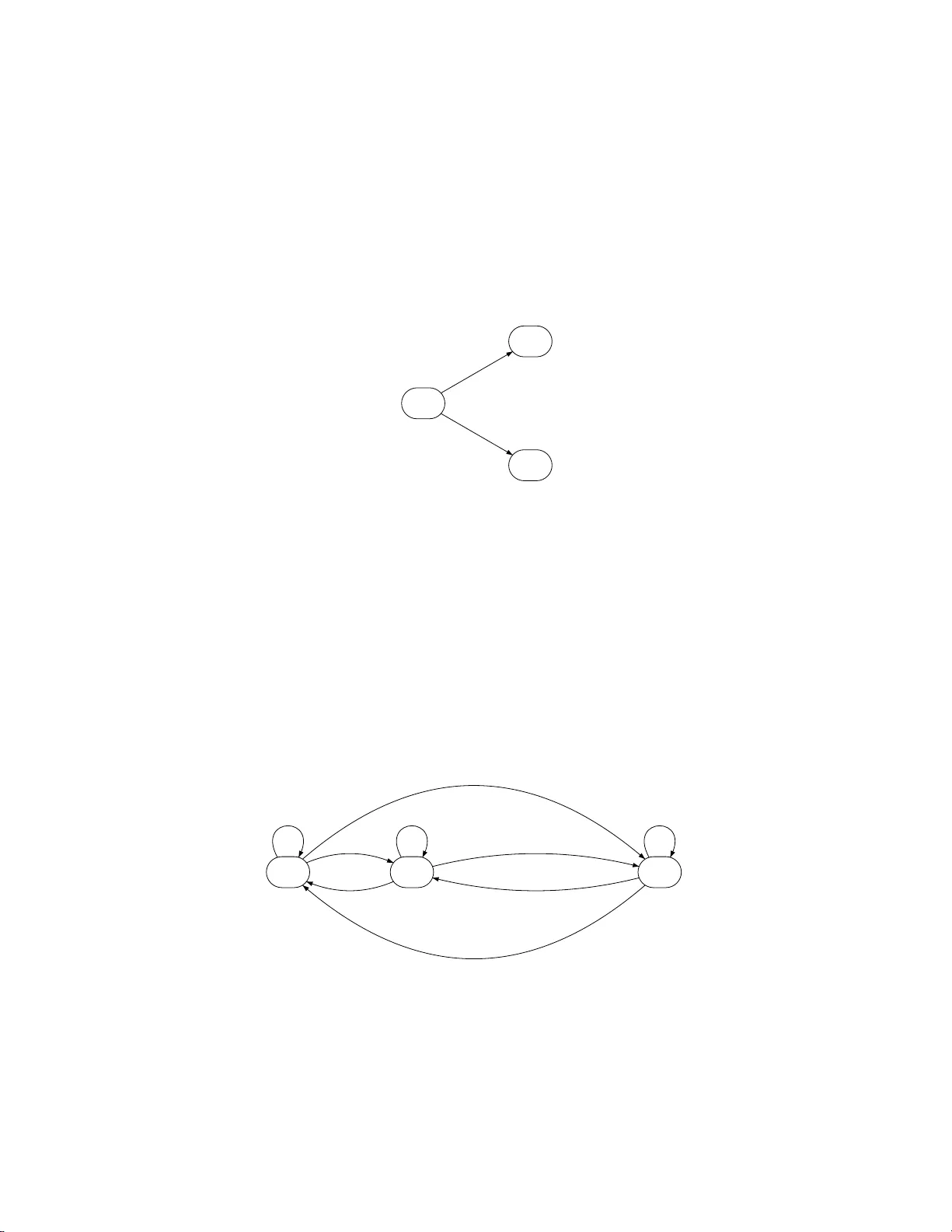
WEIGHTED A UTOMA T A AND R E CURRENCE EQUA TIONS F OR REGULAR LANGUA GES E. CAR T A-GERARDINO 1 ECAR T A-GERARDINO@YORK.CU NY.EDU P . BABAALI 2 PBABAALI@YORK.CUNY .EDU 1 , 2 DEP AR TMENT OF MA THEMA TICS AND COMPUTER SCIENCE YORK COLLEGE, CITY UNIVERSITY OF NE W YORK 94-20 GUY R. BREWER BOULEV ARD, JAMAICA, NEW YORK 11451 UNITED ST A TES Abstract. Let P (Σ ∗ ) b e the semiring of languages, and consider its subset P (Σ). In t his paper we define the language recognized by a weigh ted automa- ton ov er P (Σ) and a one-letter alphabet. Simi larly , we in troduce the notion of language recognition by l inear recurrence equations with co efficien ts in P (Σ). As w e will see, these tw o defin itions coincide. W e prov e that the languages rec- ognized by linear recurrence equations with co efficient s in P (Σ) are pr ecisely the regular languages, th us providing an alternative w ay to present these l an- guages. A remark able consequ ence of this kind of recognition i s that i t induces a partition of the language i n to its cross-sections, where the n th cross-s ection con tains all the words of length n in the language. Finally , we show how to use l inear r ecurr ence equations to calculate the density f unction of a regular language, whi c h assigns to every n the num ber of w ords of l ength n in the language. W e also show ho w to count the num b er of successful paths of a we ighted automaton. Keywor ds: cross-section of a language, density of a language, language recog- nition, recurrence equations, semir ings, weigh ted automata 1. Introduction W eighted automata are p ow erful finite-state ma chines in whic h every tra nsition carries a weight from a s emiring. These automata hav e bee n studied r ecently in a wide rang e of settings, from very applied fields, like na tural la ng uage and sp eech- pro cessing (see [1 1, 10, 9]), to more theo retical ones, like logic (see [5]) . In our current resear ch, we ar e par ticularly interested in the applicatio ns of weighted a u- tomata to for ma l lang uage theor y . A finite auto maton ([6, 7]) ca n b e regarded as a particular type o f w eig ht ed automaton, by letting the weigh ts come from the Bo ole an semiring (i.e., the weigh ts are either 0 or 1). Thus, the c lass of weighted automata co n tains the c lass of finite automata. Kleene’s Theorem states that finite automata recognize the reg ular languages . Hence, it is no surprise that w eighted automata ca n be used to recognize a class of languages that co n tains the cla ss of the regular langua ges. In particula r, it can b e sho wn tha t weigh ted automata can be used to recog nize co nt ext-free languages (see [4]). 1 2 E. CAR T A-GERARDINO & P . BABAALI In our w ork we are interested in weigh ted automa ta ov er a one-letter alphab et. W e r e fer to these automata as counting auto mata, since they ca n b e used as count- ing devices, with a pplications in combinatorics a nd enum era tio n (see [12, 1 3, 14]), among others. W e start by recalling th e definitions of a semiring and a formal power series (Section 2). These notions pro vide the settin g w e need to a s so ciate a linear recurrence eq uation t o eac h state of a counting automaton. In fact, w e will see that a counting automaton ov er a semiring K generates a s ystem of linea r recurrence equations with co efficients in K (S ection 3). Given our interest in the applica tions of weigh ted a utomata to formal languag e theory , we explore c ountin g automata, and recurr e nce equations, ov er the semiring of languages , P (Σ ∗ ) (Section 4). Spec ific a lly , we consider its subset P (Σ). W e define the language re cognized by a count ing automaton ov er P (Σ), and in tro duce the idea o f la nguage r ecognition by linear recurrence equations with co efficients in P (Σ). W e will see tha t these tw o types of language r e cognition a re equiv a lent. A consequence of recognizing a language this way is that we o bta in a partition of the languag e into its cr oss-se ctions , where the n th cross - section co n tains all the words of length n in the la nguage (see [2, 1 ]). It is imp or tant to notice that this is the case b ecause the weigh ts of the automata a nd the co efficients of the recur rence equations come from P (Σ). W e will show that the la nguages recog nize d b y co unt ing automata over P (Σ), and by linear recurre nce equations with co efficients in P (Σ), are closed under certain o per ations. W e then prove that a lang uage r e c ognized by a system of linear re currence equations with co efficients in P (Σ) is r egular, a nd that every regular languag e is r ecognized by a system o f linear recurrence equa tions with co efficients in P (Σ). This re sult provides a novel wa y to presen t this impo rtant cla ss of lang uages. W e conclude this pa per by showing how to use linea r recurr ence equations to count, for every n , the n umber of words of leng th n in a regular lang uage (Section 5). That is, w e show ho w to calculate the density funct ion o f the langua g e (see [15]). W e will see tha t the num b er of words of le ngth n in a languag e is closely related to the num b er of successful paths o f length n in the co un ting automato n recognizing the languag e. Th us , we s ta rt by counting the num b er of succ e s sful pa ths of any given length in an automaton. W e do this by constr ucting an automaton that co un ts the num b er of successful paths of another automaton. W e refer to this machine as a path-counting a utomaton, and we use it to construct the se lf- c o unt ing a utomaton, which w e will define as a machine with the ability to count its own succes sful paths. Therefore, for every n , we hav e a wa y to ( i ) gener ate all the words o f length n and to ( ii ) co unt the num ber of words of length n in a regular language. 2. Preliminaries: Semirings and Formal Powe r Series A m o noid is a nonempty s et on whic h we define an asso c ia tive o pe r ation, a nd in which ther e is an identit y ele men t. Using this, we ca n define a semiring . Definition 2.1. A semiring K = ( K, + , · , 0 , 1) is a set K satisfying (1) ( K, + , 0) is a commutativ e monoid with identit y element 0 (2) ( K, · , 1) is a monoid with identit y element 1 (3) for a ll a, b, c in K , a · ( b + c ) = a · b + a · c (4) for a ll a in K , 0 · a = a · 0 = 0 WEIGHTED AUTOMA T A & RE CURRENCE EQUA TIONS FOR REGULAR LANGUA GES 3 F rom the definition we can see that every r ing with unity is a s emiring. (F or example, the ring of the rea l num ber s is a n example of a semir ing.) Some nontrivial examples of semirings are the semiring of natural n umbers N = ( N , + , · , 0 , 1), the Bo olean sem iring B = ( { 0 , 1 } , ∨ , ∧ , 0 , 1), and the sem iring of languages P (Σ ∗ ) = ( P (Σ ∗ ) , ∪ , · , ∅ , { ε } ), where Σ is a finite alphab et , Σ ∗ is the set o f all wor ds of finite leng th over Σ ( ε denotes the empt y word), and P (Σ ∗ ) is the p ow er set of Σ ∗ , k nown as the s e t of languages over Σ. It is not difficult to see that if K 1 and K 2 are t wo semirings, then their direct pro duct K 1 × K 2 is also a semiring. Definition 2.2. Let A b e a finite alphab et and K a semiring. W e can define a map s : A ∗ → K , as signing to ev ery word w ∈ A ∗ an element c ∈ K . Such a map is known a s a formal p ow er s eries . W e call s ( w ) = c the c o efficient of w , or the weight of w . Of course , these co efficients or weigh ts hav e different interpretations, dep ending on the particular semiring K . The set of all formal p ow er series s : A ∗ → K is usually denoted by K hh A ∗ ii . F or example, if A is a finite alphab et a nd K = B , then notice that for w ∈ A ∗ , s ( w ) is either 0 or 1 (false or tr ue, resp ectively). Hence, a formal p ower series s ∈ B hh A ∗ ii r ejects or a c cepts a word w ∈ A ∗ . W e hav e seen that, given a semiring K (and a finite alphab et A ), we can define the set of formal p ow er ser ies K hh A ∗ ii . In turn, the set of for mal p ow er series can be made into a semir ing in the following wa y ([8]). Addition of tw o ser ies s 1 , s 2 ∈ K hh A ∗ ii is defined b y ( s 1 + s 2 )( w ) = s 1 ( w ) + s 2 ( w ), for all w ∈ A ∗ . The series defined by 0 ( w ) = 0 is the identit y for the a ddition. Multiplication of tw o series s 1 , s 2 is defined b y ( s 1 · s 2 )( w ) = X w 1 w 2 = w ( s 1 ( w 1 )) · ( s 2 ( w 2 )), for all w ∈ A ∗ . (This op eration is known as the Cauchy pro duct of tw o formal p ow er se ries.) The ident ity for the pro duct is the series ε ε ε defined by ε ε ε ( ε ) = 1, while ε ε ε ( w ) = 0 for any other w ord w 6 = ε . Hence, ( K hh A ∗ ii , + , · , 0 , ε ε ε ) is a semiring , the semiring of formal p ow er s eries . 3. Weighted Automa t a and Recurrence Equa tions A convenien t wa y to represent some for mal p ow er series is by means o f weigh ted automata ([5]). Definition 3.1. Let K = ( K , + , · , 0 , 1) b e a semiring and A a finite alphabe t. A w eighted automaton A ov er K and A is a quadruple A = ( Q A , ι, τ , ϕ ), where Q A is a finite set of s tates, ι, ϕ : Q A → K a re functions defining the initial w eight and the final w eight of a state, res p ectively , and if n is the n umber of states, τ : A → K n × n is the transition weigh t function. W e let τ ( x ) be an ( n × n )-matr ix whose ( i, j )-en try τ ( x ) i,j ∈ K gives the weigh t o f the transition q i x − → q j . If τ ( x ) i,j = a , w e denote this by q i x | a − → q j . Notice that the definition of a weigh ted automaton do es not include the notions of initial or final states . Ho wev er, b y appropriately defining ι and ϕ , it is pos s ible to eq uip a weigh ted automaton with initial and final states, as we w ill see later on. Consider now the path P : q 0 x 1 | a 1 − → q 1 x 2 | a 2 − → q 2 − → . . . − → q n − 1 x n | a n − → q n in A . Denote the leng th of the path by | P | . Now define the w eight of the path by k P k = ι ( q 0 ) · a 1 · a 2 · · · a n · ϕ ( q n ) . 4 E. CAR T A-GERARDINO & P . BABAALI Notice that this path has as lab el the word w = x 1 x 2 . . . x n ∈ A ∗ . There might be, of course, other paths with lab el w = x 1 x 2 . . . x n . W e will define the w eight of the word w in A to b e the sum of the w eights k P k over all paths P with lab el w . Denote this by kAk ( w ), a nd notice that the weight of a word w in A is a function from A ∗ to K . That is, kAk is a formal p ow er series, so k Ak ∈ K hh A ∗ ii . A for mal p ow er series s ∈ K hh A ∗ ii is said to b e automata r e c o gnizable if there is a weigh ted automaton A such that s = kAk . In this case we say tha t A is an automata r epr esent ation for s ∈ K hh A ∗ ii . In our resear ch w e are interested in automata ov er a one-letter alphab et A = { x } . Hence, a typical path in such an automa to n is P : q 0 x | a 1 − → q 1 x | a 2 − → q 2 − → . . . − → q n − 1 x | a n − → q n . Given that every tr ansition reads the le tter x , we eliminate it fr om the dia g ram for simplicit y , thus making a typical path loo k like P : q 0 a 1 − → q 1 a 2 − → q 2 − → . . . − → q n − 1 a n − → q n . Since A = { x } , a n arbitr ary word w ∈ A ∗ has the form w = x n for some n ∈ N . B y definition, kAk ( w ) = kAk ( x n ) equals the s um of k P k ov er all paths P with lab el w = x n . But since e very tr a nsition rea ds the letter x , kAk ( x n ) equa ls the sum of k P k over a ll pa ths P of length n . W e call kAk the b eha vior o f the automaton A , and define it a s kAk ( x n ) = X P {k P k : | P | = n } . Note that in this kind of automaton we ar e not dir ectly a c c epting/rejecting words ov er some alphab et, but ra ther coun ting paths of length n , and k eeping track of the weigh ts of s uch paths. The idea of using a utomata a s counting devices has b een used recently w ith a pplica tions in combinatorics and difference equa tions [12, 13, 14]. Thus, we refer to weighted a utomata over a one-letter a lphab et as coun ting automata . In our work, we further explore so me of the prop erties of counting automata. Suppo se w e are interested in c o mputing the w eight of all paths of length n (equiv alently , all paths with lab el x n ) in an automato n A , star ting at a sp ecific state q 0 . Then w e would lo ok at all paths of length n starting a t q 0 , co mpute the weigh t of ea ch of these paths, and add up these weigh ts. W e call this the b eha vior of the state q 0 and deno te it by kAk q 0 . Then kAk q 0 ( x n ) = X P {k P k : | P | = n and P starts at q 0 } . Notice that, given any state q 0 , kAk q 0 ∈ K hh{ x } ∗ ii ∼ = K N . Since kAk q 0 assigns to every word x n an e le ment c n ∈ K , we can identify kAk q 0 : x n 7→ c n with a function f 0 : n 7→ c n . Hence, in a counting automaton, every state q 0 generates a function f 0 ∈ K N , a nd thus we ca n identify ea ch state with the function it genera tes. The idea of asso cia ting a function to each state of an a utomaton go es back to c lassical automata theor y (se e [3, 6]). In what follows, we will assume that the initial weigh ts of the states o f an au- tomaton A ar e either 0 o r 1. Those with a weight of 1 will b e the initia l s tates, and thos e with a weigh t of 0 will b e non-initial. Denote the set of initial states by I A . F o r the momen t, supp ose that I A = Q A , so that every state is allow ed to b e an initial state. In the next se c tion we will assume that I A ( Q A . W e will a llow more freedo m to the wa y we define the fina l weigh ts of the sta tes o f an automato n. WEIGHTED AUTOMA T A & RE CURRENCE EQUA TIONS FOR REGULAR LANGUA GES 5 Those states with a non-zero weigh t will b e the final states, and those with a weigh t of 0 will b e non-final. W e will denote the set of final s tates by F A . Now consider an arbitrar y state f 0 ∈ Q A . Let { f 1 , . . . , f k } be the set of states that ca n b e r eached fro m f 0 through paths o f length 1, with transition weigh ts a 1 , . . . , a k , r esp ectively . Supp ose that the final weigh t of state f 0 is c 0 , a nd that the final weight s o f s tates f 1 , . . . , f k are c 1 , . . . , c k , resp ectively . A gra phica l repre- sentation of this is f 0 /c 0 f 1 /c 1 . . . f k /c k a 1 a k Figure 1. Paths of length 1 starting at sta te f 0 Let f 0 ∈ K N be the function gene r ated by state f 0 , and let f 1 , . . . , f k ∈ K N be the functions gener a ted b y states f 1 , . . . , f k , r esp ectively . It can b e shown (see [12]), that (3.1) f 0 (0) = c 0 , f 0 ( n + 1) = a 1 f 1 ( n ) + a 2 f 2 ( n ) + . . . + a k f k ( n ) , for n ≥ 0 . Notice that E qs. 3.1 provide a recursive definition of the function gener ated by each state o f a counting automaton. U sing this, it can b e shown that a counting automaton A ov er K g enerates a system of linear recurrence equatio ns . And by definition, these a r e the only equatio ns re c ognized by A . Theorem 3. 1. ( [12] ) Su pp ose that A is a c ounting aut omaton over a semiring K . f 1 /c 1 f 2 /c 2 . . . f k /c k a 11 a 22 a kk a 12 a 21 a 2 k a k 2 a 1 k a k 1 The functions f 1 , f 2 , . . . , f k ∈ K N gener ate d by A satisfy the fol lowing system of line ar r e curr enc e e quations. (3.2) f i ( n + 1) = k X j =1 a ij f j ( n ) , f i (0) = c i , 1 ≤ i ≤ k 6 E. CAR T A-GERARDINO & P . BABAALI Conversely, given this system of line ar r e curr enc e e qu ations, the c ount ing automa- ton r e c o gn izing it is pr e cisely A . Example 3.1. Higher- Deg ree Systems Consider the following system of linear rec urrence equations ov er a n a rbitrary semiring K . f 1 ( n + 4) = a 12 f 2 ( n ) , f 1 (0) = c 1 f 2 ( n + 1) = a 21 f 1 ( n ) + a 22 f 2 ( n ) , f 2 (0) = c 2 Note that the degree of f 1 is 4. Theorem 3.1 guara nt ees that we can build a n automaton recognizing equa tio ns of degr ee 1. In order to use this result, we need to intro duce additional functions that act as int ermedia te states . The functions we need ca n b e defined as follows. g 1 ( n + 1) = f 1 ( n + 2) , g 1 (0) = f 1 (1) = d 1 g 2 ( n + 1) = f 1 ( n + 3) , g 2 (0) = f 1 (2) = d 2 g 3 ( n + 1) = f 1 ( n + 4) , g 3 (0) = f 1 (3) = d 3 Using these auxiliar y functions, we can rewrite the or iginal sys tem of equatio ns as a sy s tem of equatio ns of degree 1. f 1 ( n + 1) = g 1 ( n ) g 1 ( n + 1) = g 2 ( n ) g 2 ( n + 1) = g 3 ( n ) g 3 ( n + 1) = a 12 f 2 ( n ) f 2 ( n + 1) = a 21 f 1 ( n )+ a 22 f 2 ( n ) Now we can use Theor em 3.1 to build the a utomaton that re c o gnizes the given system o f linear recur rence equa tions. f 1 /c 1 g 1 /d 1 g 2 /d 2 g 3 /d 3 f 2 /c 2 a 22 1 1 1 a 12 a 21 Figure 2. Automaton r e c ognizing the sys tem of recur rence equa- tions in Example 3.1 Theorem 3.1 a b ove shows that a coun ting automaton ov er a s e miring K gener ates a system o f linear r e currence equations with coefficients in K . In the next sec tio n we will restr ict our a tten tion to the case wher e K = P (Σ ∗ ). Specifica lly , we will consider its subset P (Σ). O ur g oal is to define the language recognized by a counting automaton over P (Σ), and to define what it means for a la ng uage to b e re cognized by a system of linea r recurr ence equa tio ns with co efficien ts in P (Σ). One of the implications of defining languages this way is that we obtain an immediate pa rtition of the lang uage into its cr oss-sec tions. W e will see that it is also p oss ible to define these langua ges throug h formal gra mmars, and w e will show that these languag es are c lo sed under union, conca tenation, a nd the Kleene star. Using this, we will prov e that the langua ges re cognized b y linear recurrenc e equations with co efficients in P (Σ) are precisely the regular lang uages. WEIGHTED AUTOMA T A & RE CURRENCE EQUA TIONS FOR REGULAR LANGUA GES 7 4. Language Recognition, L anguage P ar tition, and the Cr oss-Sections of a Regular Language In this section, the semiring we use fo r the w e ights of the automata and for the co e fficie n ts o f the recurrence e q uations is P (Σ ∗ ). In pa rticular, we will o nly consider weights a nd co efficients in P (Σ) ⊂ P (Σ ∗ ). Suppo se that A is a counting automaton with weight s in P (Σ), and ass ume that the set of states of A is { f 1 , f 2 , . . . , f k } . As it is customary when us ing automata for language r ecognition, w e will assume that there is only one initial state. Without loss of generality , we will let the first state be the initial state. Therefore, I A = { f 1 } . W e now sp ecify the final weigh ts of the states in A . Non-final s tates were defined as states that hav e a final weigh t of 0; in the semiring of la nguages, ∅ . Final states were defined as s tates with a non-zero final weigh t. Sp ecifica lly , we will a s sume that the final states hav e a final weight of 1 ; in the semiring of lang ua ges, { ε } . Therefore, f i (0) = ∅ if f i / ∈ F A , and f i (0) = { ε } if f i ∈ F A . Let A b e a counting automa ton with k states f 1 /c 1 f 2 /c 2 . . . f k /c k L 11 L 22 L kk L 12 L 21 L 2 k L k 2 L 1 k L k 1 Figure 3. Counting automaton A over P (Σ) ⊂ P (Σ ∗ ) where I A = { f 1 } , c i = { ε } if f i ∈ F A , c i = ∅ if f i / ∈ F A , and for every i and every j , L ij ∈ P (Σ). (If L ij = ∅ , we can eliminate this transitio n from the diagram.) W e know that f 1 , the initial state, generates a function f 1 : N → P (Σ ∗ ) defined by the system (4.1) f i ( n + 1) = k [ j =1 L ij · f j ( n ) , f i (0) = c i , 1 ≤ i ≤ k . Since L ij ∈ P (Σ), we have that for every n ∈ N , f 1 ( n ) is a la nguage containing words o f length n . Denote f 1 ( n ) b y L n . Definition 4. 1. The language recognized by a counting autom aton A ov er P (Σ) is denoted by L A and is defined by L A = [ n L n . Thu s, a word w of length n b elong s to L A if w b elong s to L n . W e will say that a word w o f length n is reco gnized by the co un ting automaton A if there is a pa th of leng th n starting at f 1 and ending a t a final state with weigh t { w } . 8 E. CAR T A-GERARDINO & P . BABAALI Given that the languages L n are defined recursively , we c an also define the language [ n L n in the fo llowing way . Definition 4.2. L = [ n L n is k nown as the language recogni zed b y l inear recurrence equations , s ince the langua ges L n are defined via linear r e currence equations. R emark. A consequence o f reco gnizing a language L via linear recurrence equations with co efficients in P (Σ) is that the langua g e is automatically partitioned into s e ts L n , wher e L n contains all the words of length n in L , i.e., L n is the n th cross- section of the langua ge. Since the oper a tions of the semiring of languages are union and concatenation, it is no t difficult to see tha t we can also define L A by using a gra mmar. W e asso c ia te a nonterminal sy m b ol A i to every sta te f i , except that we denote A 1 by S , the start symbol, since f 1 is the initial s tate. The set of terminal symbols is Σ. Cons ider an arbitrar y transitio n f i L ij − → f j and suppo se that L ij = { a ij, 1 , a ij, 2 , . . . , a ij,m } is non- empt y . Then to this transition we a sso ciate the pro ductions A i → a ij, 1 A j , A i → a ij, 2 A j , . . . , A i → a ij,m A j . Finally , for every state f i ∈ F A (so f i (0) = { ε } ) we include a pro duction A i → ε . Denote this grammar by G A . Then we will also define L A by L A = L ( G A ). W e now present the closure prop er ties of these languages . Theorem 4.1. The languages r e c o gnize d by c ounting automata over P (Σ) ar e close d under un ion, c onc atenation, and t he Kle ene star. Pr o of. Assume that L A and L B are the languages recognized by A and B , r esp ec- tively , where A and B are co un ting a utomata ov er P (Σ). W e will show that we can construct counting automata ov er P (Σ) tha t reco gnize L A ∪ L B , L A · L B , and L ∗ A . Let Q A = { f 1 , f 2 , . . . , f k } be the set of s tates of A . Assume that I A = { f 1 } and that F A is the (none mpty) set of final states of A . Then we know that L A is recognized by a n automaton like th e o ne in Figure 3, with weigh ts L A ij , for 1 ≤ i, j ≤ k . Similar ly , let Q B = { g 1 , g 2 , . . . , g m } b e the set of states of B . Supp ose that I B = { g 1 } a nd that F B is the (nonempt y) s e t o f final states of B . Then L B is also r ecognized by an automaton like the one in Figur e 3 , but with weights L B ij , for 1 ≤ i, j ≤ m . W e first construct an automaton C reco g nizing L A ∪ L B . Le t Q C = { h } ∪ Q A ∪ Q B and I C = { h } . W e let F C = { h } ∪ F A ∪ F B if f 1 ∈ F A or g 1 ∈ F B . O therwise, F C = F A ∪ F B . Now we just need to sp ecify the transitions. The new automaton C will contain all the transitio ns in A and in B , plus s ome new ones. F or every transition f 1 L A 1 j − → f j , 1 ≤ j ≤ k , w e add a new tra nsition h L A 1 j − → f j . Similarly , for every tra nsition g 1 L B 1 j − → g j , 1 ≤ j ≤ m , we add a new tr a nsition h L B 1 j − → g j . Then C recognizes L A ∪ L B . Tha t is, L C = L A ∪ L B . W e now constr uc t an auto maton C that recognizes L A · L B . Let Q C = Q A ∪ Q B and I C = { f 1 } . W e let F C = { f 1 } ∪ F B if f 1 ∈ F A and g 1 ∈ F B . O therwise, F C = F B . As for the tr ansitions in C , we will include all the transitions in A a nd in B , as well as some other one s . Ass ume that F A = { f j 1 , f j 2 , . . . , f j l } . Then, for every state f i , 1 ≤ i ≤ k , given the tr a nsitions f i L A ij 1 − → f j 1 , f i L A ij 2 − → f j 2 , . . . , f i L A ij l − → f j l , we add a WEIGHTED AUTOMA T A & RE CURRENCE EQUA TIONS FOR REGULAR LANGUA GES 9 new tr ansition f i L A i − → g 1 , where L A i = L A ij 1 ∪ L A ij 2 ∪ . . . ∪ L A ij l . Finally , if f 1 ∈ F A , then for ev ery tra nsition g 1 L B 1 j − → g j , 1 ≤ j ≤ m , w e a dd a tr ansition f 1 L B 1 j − → g j . By construction, we conclude tha t L C = L A · L B . W e conc lude the pr o of by co nstructing an automaton C that re cognizes L ∗ A . Let Q C = { h } ∪ Q A , I C = { h } , a nd F C = { h } ∪ F A . The automaton C w ill contain all the tra nsitions in A , plus some new ones. F or each state f j , 1 ≤ j ≤ k , given the transition f 1 L A 1 j − → f j , we add a transition h L A 1 j − → f j , a nd for ev ery f i ∈ F A , we also add tra nsitions f i L A 1 j − → f j (to the state f j ). Then L C = L ∗ A .  By combining Theo rems 3.1 a nd 4.1, we obtain the following. Corollary 4.2. The languages r e c o gnize d by systems of line ar r e curr enc e e quations with c o efficients in P (Σ) ar e close d under union, c onc atenation and the Kle ene star. W e are now ready to prov e one of our ma in results. Theorem 4.3. A language r e c o gnize d by a syst em of line ar r e curre nc e e quations with c o efficients in P (Σ) is r e gular. Conversely, every r e gular language is r e c o gnize d by a system of line ar r e cu rr enc e e qu ations with c o efficients in P (Σ) . Pr o of. Suppo se that L is a language reco g nized by a system of linear recur r ence equations with co efficie nts in P (Σ). Then we know that there is a counting au- tomaton A ov er P (Σ) such that L = L A . By de finitio n, L A is gener ated by the grammar G A provided b efore Theorem 4 .1. Note that this gr ammar is r egular. Therefore, L is a reg ular languag e. Now we need to show that if a languag e is regular , then it is recognized by a system of line a r rec ur rence eq uations with co efficients in P (Σ). Recall that the set o f regular languages over an alphabet Σ = { a 1 , a 2 , . . . , a m } is defined by ( i ) ∅ , { ε } , { a 1 } , { a 2 } , . . . , { a m } are regular, and ( ii ) if L 1 , L 2 are r e g ular, then L 1 ∪ L 2 , L 1 · L 2 , and L ∗ 1 are regular. It is not difficult to find systems of linear recurrenc e equations with co efficients in P (Σ) that r e cognize the lang uages in ( i ). Note that (4.2) f 1 ( n + 1) = ∅ · f 1 ( n ) , f 1 (0) = ∅ recognizes ∅ , (4.3) f 1 ( n + 1) = ∅ · f 1 ( n ) , f 1 (0) = { ε } recognizes { ε } , a nd (4.4) f 1 ( n + 1) = ∅ · f 1 ( n ) ∪ { a i } · f 2 ( n ) , f 1 (0) = ∅ f 2 ( n + 1) = ∅ · f 1 ( n ) ∪ ∅ · f 2 ( n ) , f 2 (0) = { ε } recognizes { a i } , for each a i ∈ Σ. Finally , supp ose that L 1 and L 2 are tw o languages recognized by s ystems of linear r ecurrence equations. By Coro llary 4.2, there are systems of linear rec ur rence equa tions r ecognizing L 1 ∪ L 2 , L 1 · L 2 , and L ∗ 1 .  Theorem 4 .3 shows that linear recur rence equations with co efficients in P (Σ) recognize, pr ecisely , the regular languages . Hence, co unting a utomata over P (Σ) recognize the regula r languag es as well. By Kleene’s Theorem, reg ula r languages are reco gnized by finite automata. Thus, it is na tur al to translate c o ncepts from finite automata theory to counting a utomata o ver P (Σ). F or example, we can define what it means for a counting automato n ov er P (Σ) to b e deterministic. 10 E. CAR T A-GERARDINO & P . BABAALI Definition 4.3. Let A b e a counting automaton ov er P (Σ) and let Q A = { f 1 , f 2 , . . . , f k } b e its set of states . W e say that A is determ inistic if for every state f i , the transition weight lang uages L i 1 , L i 2 , . . . , L ik are pairwise disjoint. Note tha t this is eq uiv alent to saying that given f i ∈ Q A and a ∈ Σ, a b elongs to at mos t one of the transition weigh t lang ua ges L i 1 , L i 2 , . . . , L ik . Hence, our defi- nition coincides with the classic al definitio n of a deterministic a uto maton (s e e [6]). Notice we have not discuss e d how to turn a (nondeterministic) counting automa- ton int o a deter ministic o ne. It should b e cle a r, howev e r, that the techniques to accomplish this fr om finite automata theory can b e applied to co unt ing automa ta ov er P (Σ). Example 4.1. Recurr e nc e Equations and Regular Languag es Let L = ( ab ∗ a ) ∗ and notice that L is a regular la nguage. Assume that the alphab et is Σ = { a, b } . Then L is rec ognized by the automaton A b elow. f 1 / { ε } f 2 / ∅ { b } { a } { a } Figure 4. Counting automaton A recog nizing ( ab ∗ a ) ∗ Equiv ale n tly , L = ( ab ∗ a ) ∗ is r ecognized by the system b elow. f 1 ( n + 1) = { a } · f 2 ( n ) , f 1 (0) = { ε } f 2 ( n + 1) = { a } · f 1 ( n ) ∪ { b } · f 2 ( n ) , f 2 (0) = ∅ W e can write L as L = [ n L n , where L n = f 1 ( n ) is the n th cro s s-section o f L . I f we write the sys tem ab ov e in matrix for m, a s  f 1 ( n + 1) f 2 ( n + 1)  =  ∅ { a } { a } { b }   f 1 ( n ) f 2 ( n )  , then  f 1 ( n ) f 2 ( n )  =  ∅ { a } { a } { b }  n  { ε } ∅  . Notice that f 1 (1) = ∅ , which a grees with the fact that the la nguage ( ab ∗ a ) ∗ has no words of length 1. Similarly , f 1 (4) = { aaaa, a bba } , and no te that these are precise ly the words of length 4 in ( ab ∗ a ) ∗ . 5. P a th-Counting and Self-Counting Automa t a: Calcula ting the Density Function of a Regular Language In the pre v ious sec tion we saw how we can use weigh ted automata and linea r recurrence equations to r ecognize a r egular languag e. In pa rticular, we saw how this type o f langua ge recognitio n induces a par tition of the languag e into its c r oss- sections. And thus, for each n , we hav e a w ay of generating all the words of length n in the langua ge. In this section we will s ee that it is p ossible to output no t only the words, but also the num ber o f words, of length n in the langua ge. That is, we show how to ca lculate the density function of the langua ge. Reca ll that a word of leng th n is rec o gnized by a successful pa th with the same length. With this co nnection in mind, we start b y construc ting an automaton that can count, for any g iven n , WEIGHTED AUTOMA T A & RE CURRENCE EQUA TIONS FOR REGULAR LANGUA GES 11 the n umber of succes sful pa ths of length n . In order to do this, we introduce the notion o f a path- c o unt ing a utomaton. Definition 5.1. Giv en a counting a utomaton A , its path-coun ting automaton ¯ A is a co unting automaton over N that is able to count the num b er o f successful paths o f a ny given length in A . W e now show how to constr uct a path-c ounting automa ton ¯ A . Assume that the se t of states of A is { f 1 , f 2 , . . . , f k } . Then we denote the set of s tates of ¯ A by { ¯ f 1 , ¯ f 2 , . . . , ¯ f k } . W e let ¯ f i be a n initial state in ¯ A if f i is an initial state in A . Suppo se that ¯ f i (0) = ¯ c i . W e let ¯ c i = 1 if f i is final. Otherw is e, if f i is non-final, we let ¯ c i = 0. Fina lly , consider a transition ¯ f i ¯ a ij − → ¯ f j in ¯ A , corre s po nding to a transition f i a ij − → f j in A . W e let ¯ a ij = 1 if a ij 6 = 0 . Otherwis e , if a ij = 0 , we let ¯ a ij = 0. By Theorem 3.1, the automaton ¯ A generates a sys tem (5.1) ¯ f i ( n + 1) = k X j =1 ¯ a ij ¯ f j ( n ) , ¯ f i (0) = ¯ c i , 1 ≤ i ≤ k . F rom the wa y we defined ¯ c i and ¯ a ij , a simple pro of by induction shows that, if f i is an initial state, ¯ f i ( n ) equa ls the num b er of successful pa ths o f length n that s tart at f i . W e now define the self-counting automato n. Definition 5.2. Given a coun ting automa to n A and its corresp onding pa th- c o unt ing automaton ¯ A , the self-counting automaton  A , ¯ A  is a counting automaton ov er K × N capable of counting its own succ essful paths o f any given length. Essentially ,  A , ¯ A  is an ex tension of the automaton A . If the set of states o f A is { f 1 , f 2 , . . . , f k } , then the set o f states of  A , ¯ A  is {  f 1 , ¯ f 1  ,  f 2 , ¯ f 2  , . . . ,  f k , ¯ f k  } . If f i is an initial state, we let  f i , ¯ f i  be an initial state, and for every final state f j of A , we let  f j , ¯ f j  be a final state of  A , ¯ A  . Finally , notice tha t the w eights are also ordered pair s. It is clea r that if the weight of f i − → f j is a ij , then the weigh t o f  f i , ¯ f i  − →  f j , ¯ f j  is ( a ij , ¯ a ij ). W e can think of  A , ¯ A  as an e x tension of A , wher e the fir st co ordinate keeps track of the weights of the p aths tra versed (th us mimicking A ), while the second coo rdinate keeps tra ck of the num b er of p aths trav ersed. R emark. It is not difficult to see that path-counting and self-counting automata ca n be used to count the num b e r of success ful paths o f a weigh ted automaton ov er any alphab et, no t just a one-letter alpha be t. Since a successful path do es not depend on the alpha bet used, simply ide ntify all the letters in the a lphab et, say x 1 , x 2 , . . . , x m , with a letter x , and use counting automata . W e now return to our discussion of formal langua ges. Reca ll that a word w of length n is recognized by a coun ting automaton A if there a successful path of leng th n in A with weigh t { w } . Hence, g iven a counting automaton A , we would exp ect the num b er of words of length n in L A to be equa l to the num b er of succes s ful paths of length n in A . That is , we would exp ect the density function to b e ¯ f 1 ( n ). How ever, these tw o quantities could fail to be equal. Notice that ( i ) a path could recognize mo re than one word, a nd ( ii ) a word co uld b e recognized by more than one path. The next theore m shows how to corr ectly define the function that co un ts 12 E. CAR T A-GERARDINO & P . BABAALI the num b er of words of length n (the density of the language) a nd the conditions needed on the a uto maton. Theorem 5.1. L et A b e a deterministic c ounting automaton over P (Σ) . Then the density function of L A (the language r e c o gnize d by A ) c an b e define d via line ar r e curr enc e e quations with c o efficients in N . Pr o of. Recall tha t the function ¯ f 1 ( n ) in Eq. 5.1 counts the nu mber of successful paths of length n in A . As w e p ointed out, this quantit y need not b e equal to the nu mber of w ords o f length n in L A . First, we need to account fo r case ( i ) ab ov e, since a path could recog nize more than one word. T his is b ecause a transitio n weigh t ma y contain mor e than one letter from Σ. The rec urrence equatio ns that define the density function will b e just like the ones in E q. 5.1, except that each co efficient nee ds to count the n um b er of letters in the cor resp onding transition weigh t (instead of just b eing 0s or 1s). Given a reg ular la nguage L recognized b y a system (5.2) f i ( n + 1) = k [ j =1 L ij · f j ( n ) , f i (0) = c i , 1 ≤ i ≤ k , we define the following system of linear recurr ence equations (5.3) f i ( n + 1) = k X j =1 | L ij | f j ( n ) , f i (0) = | c i | , 1 ≤ i ≤ k , where | S | denotes the ca rdinality of a set S . It is cle a r that f 1 ( n ) is g reater than or equal to the num b er of words of length n in L A . Note that f 1 ( n ) is strictly gr eater if there is a word recognized b y mo r e tha n one success ful path. W e cla im that, since A is deterministic, no word of leng th n is recognized b y more than one successful path with the same length, and thus f 1 ( n ) gives precis e ly the num ber of words of length n in L A . (Hence, determinism will take care of c a se ( ii ) ab ov e, where a word could be recog nized b y more than o ne path.) Suppo se, on the co ntrary , that there is a word w reco gnized by more than one successful path. Since A has o nly one initial state, then there is at lea st one state f i that b oth paths share, with the pr op erty that the transition w eights leaving f i are not pairwise disjoint . This contradicts the fact that A is deterministic. Thus, we co nclude that the density function of L A is f 1 ( n ).  R emark. The density function o f a langua g e L is us ua lly denoted in the liter - ature by ρ L ( n ) (see [15]). F ormal langua ges ca n b e classified acco rding to their density . F or example, we say that a lang uage has a c onstant , p olynomial , or ex- p onential density if ρ L ( n ) = f 1 ( n ) has constant, p olyno mial, or exponential or der, resp ectively . Example 5.1. Path-Counting Automata, and a Languag e of Polynomial Density Consider the regular la nguage L = a ∗ ba ∗ ba ∗ . It easy to see tha t L is re c ognized by the co unting auto ma ton A shown b elow. (Note that A is deterministic.) WEIGHTED AUTOMA T A & RE CURRENCE EQUA TIONS FOR REGULAR LANGUA GES 13 f 1 / ∅ f 2 / ∅ f 3 / { ε } { a } { a } { a } { b } { b } Figure 5. Counting automaton A r ecognizing a ∗ ba ∗ ba ∗ It is not difficult to s ee that the s ystem that defines the density function f 1 ( n ) is the one b elow. f 1 ( n + 1) = f 1 ( n ) + f 2 ( n ) , f 1 (0) = 0 f 2 ( n + 1) = f 2 ( n ) + f 3 ( n ) , f 2 (0) = 0 f 3 ( n + 1) = f 3 ( n ) , f 3 (0) = 1 W e c o uld write this system in matr ix form, as   f 1 ( n + 1) f 2 ( n + 1) f 3 ( n + 1)   =   1 1 0 0 1 1 0 0 1     f 1 ( n ) f 2 ( n ) f 3 ( n )   . Then   f 1 ( n ) f 2 ( n ) f 3 ( n )   =   1 1 0 0 1 1 0 0 1   n   0 0 1   . Alterna tively , w e could obtain an explicit for- m ula for f 1 ( n ) in the following wa y . Notice that f 3 ( n ) = 1 for n ≥ 0, and hence f 2 ( n ) = n for n ≥ 0. Using this, we o btain that f 1 (0) = 0 and, for n ≥ 1, f 1 ( n ) = f 1 ( n − 1) + ( n − 1). Thus, if n ≥ 1 , f 1 ( n ) = n ( n − 1) 2 . W e conclude that the language a ∗ ba ∗ ba ∗ contains exa ctly n ( n − 1) 2 words o f le ngth n , for n ≥ 1. Example 5. 2. Path-Counting Automata, and a Languag e of Exp onential Density Consider again the language L = ( ab ∗ a ) ∗ from Example 4.1, recognized b y the counting automaton A in Figure 4. This automa ton is, clearly , deterministic. It is not difficult to see that the density function is defined by the following sys tem. f 1 ( n + 1) = f 2 ( n ) , f 1 (0) = 1 f 2 ( n + 1) = f 1 ( n ) + f 2 ( n ) , f 2 (0) = 0 Notice that f 1 ( n + 2) = f 2 ( n + 1) = f 1 ( n ) + f 2 ( n ) = f 1 ( n ) + f 1 ( n + 1), with f 1 (0) = 1 and f 1 (1) = 0. Hence, if F n denotes the n th Fibonacci n umber, we hav e that f 1 ( n ) = F n − 1 , for n ≥ 1. W e co nclude that if n ≥ 1, the num be r of words of length n in ( ab ∗ a ) ∗ is ϕ n − 1 − (1 − ϕ ) n − 1 √ 5 , where ϕ = 1 + √ 5 2 is the golden ratio. Ackno wledgements This work was made p oss ible, in par t, by the PSC-CUNY Grant 6011 6 -39 4 0. References [1] M. Ack erman and E. M¨ akinen. Three new algorithms for regular language enumeration. In COCOON ’09: P r o c e e dings of the 15th A nnual International Confer enc e on Computing and Combinatorics . Springer-V erlag, 2009. [2] M. Ac ke rman and J. Shalli t. Efficien t enumeration of regular languag es. In CIAA’07 : Pr o c ee d- ings of the 12th International Confer enc e on Implementation and Applic ation of Automata . Springer-V erlag, 2007. 14 E. CAR T A-GERARDINO & P . BABAALI [3] J. Brzozo wski. Der i v atives of regular expressions. Journal of the A sso ciation for Computing Machinery , 1964. [4] C. C or tes and M. Mohri. Conte xt-free r ecognition with weigh ted automata. In Pr o c e e dings of the Six th Me eting on Mathematics of La nguage, MOL 6 , 1999. [5] M. Droste and P . Gastin. W eighted automata and weigh ted logics. T echnical rep ort, Lab ora- toire de Sp ´ ecification et V´ erification, ENS de Cachan and CNRS, 2005. [6] S. Eilenberg. Au tomata, La nguages, and M achines . Academic Press, 1974. [7] B. Khoussaino v and A. Nero de. Automata The ory and its Applic ations . Bir khauser, 2001. [8] W. Kuic h and A. Salomaa. Semirings, Automata, L anguages . Springer-V erlag, 1986. [9] M. Mohr i . W eigh ted finite-state transducer algorithms an ov erview. T ec hnical repor t, A T&T Labs—Researc h, 2004. [10] M. Mohri, F. Pereira, and M. Riley . W eigh ted finite-state transducers i n speech recognition. In ISCA ITR W Autom atic Sp e e ch R e c o gnition: Chal lenge s for the Mil lennium , 2000. [11] F. Pereira and M. Riley . Sp eech recognition by composi tion of weigh ted finite automata. T ec hnical rep ort, A T&T Labs—Research, 1996. [12] J. J. M. M. Rutten. Element s of stream calculus (an extensiv e exercise in coinduction). T ec hnical rep ort, Centrum v oor Wiskunde en Informatica, 2001. [13] J. J. M. M . Rutten. Behavioral differential equations: a coinductive calculus of streams, automata, and p ow er seri es. T ec hnical rep ort, Centrum v o or Wiskunde en Informatica, 2002. [14] J. J. M. M. Rutten . Coinduct ive coun ting with weigh ted automata. T ec hnical r ep ort, Cen trum v o or Wiskunde en Informatica, 2002. [15] S. Y u. R e gular L anguages . Handb o ok of F ormal Languages, V ol. 1: W ord, Language, Gram- mar. Springer-V erlag, 1997.