Recently, fractional differential equations have been investigated via the famous variational iteration method. However, all the previous works avoid the term of fractional derivative and handle them as a restricted variation. In order to overcome such shortcomings, a fractional variational iteration method is proposed. The Lagrange multipliers can be identified explicitly based on fractional variational theory.
Deep Dive into Fractional Variational Iteration Method for Fractional Nonlinear Differential Equations.
Recently, fractional differential equations have been investigated via the famous variational iteration method. However, all the previous works avoid the term of fractional derivative and handle them as a restricted variation. In order to overcome such shortcomings, a fractional variational iteration method is proposed. The Lagrange multipliers can be identified explicitly based on fractional variational theory.
The variational iteration method [1 -4] has been extensively worked out for many years by numerous authors. Starting from the pioneer ideas of the Inokuti-Sekine-Mura method, Ji-Huan He [3] developed the variational iteration method (VIM) in (1999). In this method, the equations are initially approximated with possible unknowns. A correction functional is established by the general Lagrange multiplier which can be identified optimally via the variational theory. Besides, the VIM has no restrictions or unrealistic assumptions such as linearization or small parameters that are used in the nonlinear operators [5 -11].
In the last three decades, scientists and applied mathematicians have found fractional differential equations useful in various fields: rheology, quantitative biology, *Corresponding author, Email addresses: wuguocheng2002@yahoo.com.cn. electrochemistry, scattering theory, diffusion, transport theory, probability potential theory and elasticity [12]. Finding accurate and efficient methods for solving FDEs has been an active research undertaking. A question may naturally arise: Can we have a fractional variational method to derive approximate solutions of FDEs? Although a number of useful attempts have been made to solve fractional equations via the VIM, the problem has not yet been completely resolved, i.e., most of the previous works avoid the term of fractional derivative, handle them as restricted variation and they cannot identify the fractional Langrange multipliers explicitly in the correction function.
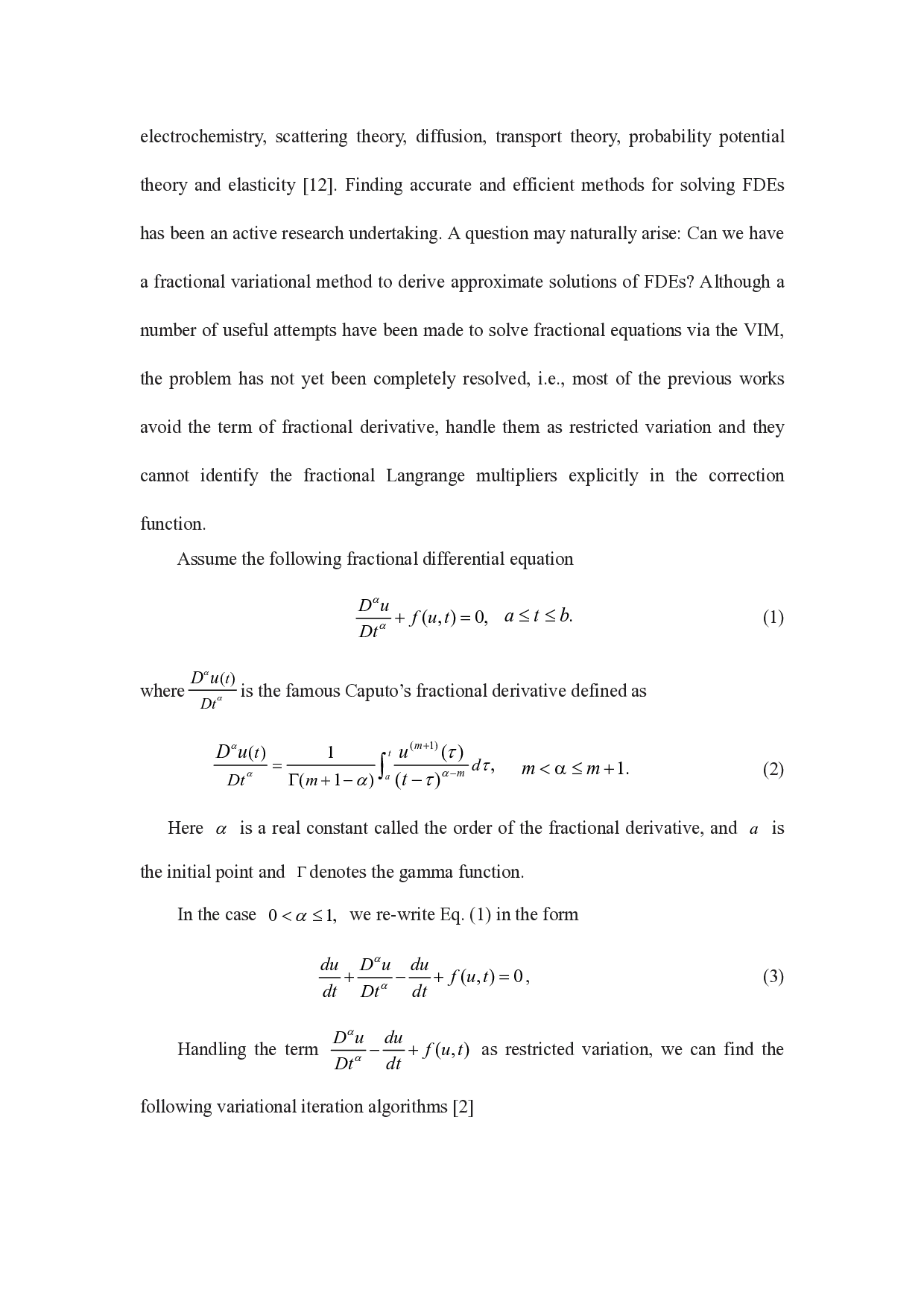
Assume the following fractional differential equation
where
is the famous Caputo’s fractional derivative defined as
( ) , ( )
Here α is a real constant called the order of the fractional derivative, and a is the initial point and Γ denotes the gamma function.
In the case 0 1 , α < ≤ we re-write Eq. ( 1) in the form
Handling the term ( , ) D u du f u t Dt dt α α -+ as restricted variation, we can find the following variational iteration algorithms [2] 1 0
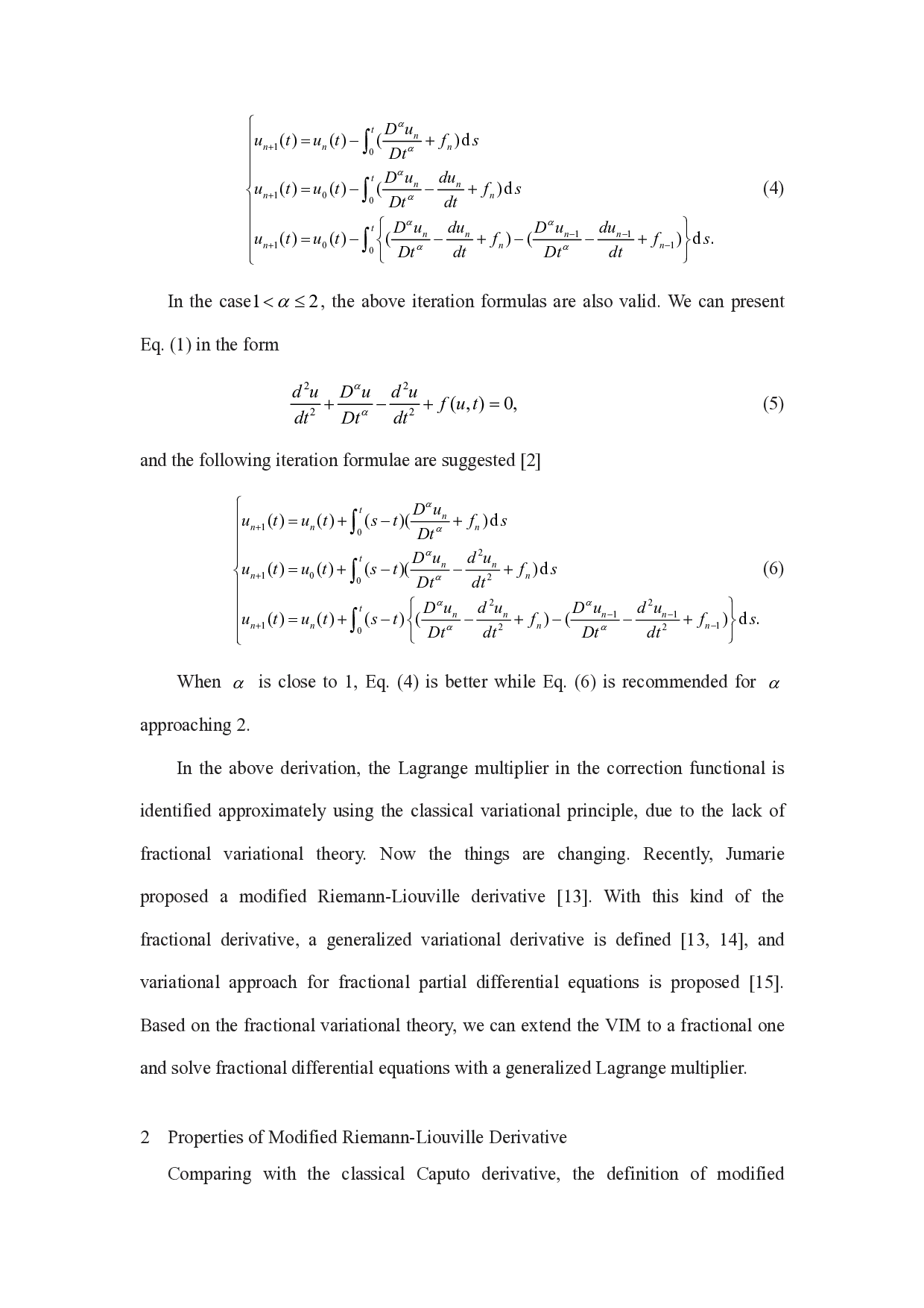
In the case1 2 α < ≤ , the above iteration formulas are also valid. We can present Eq. ( 1) in the form ( , ) 0,
and the following iteration formulae are suggested [2] 1 0
When α is close to 1, Eq. ( 4) is better while Eq. ( 6) is recommended for α approaching 2.
In the above derivation, the Lagrange multiplier in the correction functional is identified approximately using the classical variational principle, due to the lack of fractional variational theory. Now the things are changing. Recently, Jumarie proposed a modified Riemann-Liouville derivative [13]. With this kind of the fractional derivative, a generalized variational derivative is defined [13,14], and variational approach for fractional partial differential equations is proposed [15].
Based on the fractional variational theory, we can extend the VIM to a fractional one and solve fractional differential equations with a generalized Lagrange multiplier.
Comparing with the classical Caputo derivative, the definition of modified Reimann-Liouville derivative is not required to satisfy higher integer-order derivative thanα . Secondly, th α derivative of a constant is zero. Now we introduce some properties of the fractional derivative. Assume :
The modified Riemann-Liouville derivative is defined as [14] 0 0
In the next sections, we will use the following properties.
(a). Fractional Leibniz product law [13] ( ) ( ) ( ) 0 ( ) = .
x D uv u v uv
(b). Fractional integration by parts [13] ( )
(c). Integration with respect to ( )
We use the following equality for the integral w. r. t ( )
In order to propose a FVIM for fractional nonlinear equations, firstly, we should consider fractional variational theory which is employed to construct a fractional correction functional, then we need to identify the fractional Lagrange multipliers.
Several versions of fractional variational approaches have been proposed [15 -17].
However, all of them can not applied to establish a fractional variational functional for fractional differential equations. With Jumarie’s fractional derivative [13 -15], we can readily establish a generalized fractional functional. We now generally revisit the derivation of the fractional variational derivative [13,14]. Start from the functional
so that by substituting Eqs. ( 13) and ( 14) into Eq. ( 12), for each ( ) x η , we have
Note that [ ] J ε is a function of ε only and it attains its extremum at = 0 ε . Differentiating Eq. ( 15) with respect to ε gives
so that a necessary condition for ( ) J ε to have an extremum is for / dJ dε to vanish for all admissible ( ) x η which leads to the result
The integral in Eq. ( 17) can be rewritten, using the fractional Leibniz formula and integration by parts, in the form
so that we have
As ( ) x η is arbitrary, the Euler-Lagrange equation for the fractional variational principle is
Similarly, we can derive higher order fractional Euler-Lagrange equation
When 1 α = , Eq. ( 21) can turn out to be the Euler-La
…(Full text truncated)…
This content is AI-processed based on ArXiv data.